STATISTICAL METHODS FOR DATA FROM CASE-COHORT STUDIES
Poulami Maitra
A dissertation submitted to the faculty at the University of North Carolina at Chapel Hill in partial fulfillment of the requirements for the degree of Doctor of Philosophy in the
Department of Biostatistics in the Gillings School of Global Public Health.
Chapel Hill 2018
Approved by:
Jianwen Cai
Chirayath Suchindran Donglin Zeng
c
ABSTRACT
Poulami Maitra: Statistical Methods for Data from Case-Cohort Studies (Under the direction of Jianwen Cai)
In epidemiological studies and disease prevention trials, interest often lies in the relation-ship between certain disease endpoint and some exposure of interest. When the event is rare and/or some of the covariate information are quite expensive to collect for the entire cohort, case-cohort designs are widely used to reduce the financial cost of the study while achieving the same study goals. The case-cohort sampling scheme entails the random sampling of indi-viduals, called the sub-cohort, along with all the cases. In the situation when the event rate is not low but resources are limited, the generalized case-cohort design is more appropriate, where only a fraction of cases are sampled along with the sub-cohort. In this dissertation, we consider two aspects of case-cohort studies. One is for statistical methods for the analysis of recurrent events and the other concerns power/sample size calculation for interaction test.
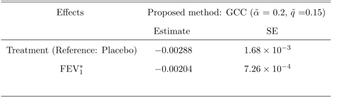
performed well. For the multiplicative rates model, we illustrated the proposed method to assess the relationship between prior measles infection and acute lower-respiratory-infections (ALRI) in a double-blinded randomized clinical trial, conducted in Brazil. We illustrated our proposed method for additive rates model to study the effect of FEV1 on the recurrence of pulmonary exacerbation in patients with cystic fibrosis.
ACKNOWLEDGEMENTS
Knowledgeable people of the internet have blogged about what to write in one’s thesis acknowledgment (yes, you read that right) and so, following them, I am going to (try to) make it short and just mention the few things and people that affected and shaped me during my time at UNC. If I had to describe my PhD experience at UNC in a single sentence, I would quote Glen Hansard, “It’s gonna be a long one/ I’ll be working all night long/ It’s gonna be a long one/ But I’m paying my way”. Even though my diploma would say PhD (Biostatistics), I’ve gotten a degree in life lessons.
Well, we are all social animals and I am no exception. These five years were spent in the presence of some amazing people, who have helped me grow as a person and a researcher. The least I can do, is mention their names. The first would be my adviser, Dr. Jianwen Cai. I am forever grateful to her for helping me with everything, whether it is my dissertation, or dealing with frustrations, or even allowing me to stay in Charlotte with Pourab. I am also indebted to all my other committee members (Dr. Suchindran, Dr. Zeng, Dr. Zhou and Dr. Bensen) for being so helpful with the dissertation. I would like to thank my parents and my parents-in-law for freaking out about every little thing in my (our) life, trying to solve them from eight thousand miles away and irrevocably supporting me through everything.
thankful to Sayan, Ritwik, Abhishek, Sujatro, Monica, Suman, Arkopal and Priyam for the happy memories, school and college friends whose conversations have always been like a breath of fresh air and Birgitte, for being there. And to our 6 month old puppy Luna, thank you for teaching me patience and that love is unconditional. Finally (almost), I would like to thank my baby sister for keeping me updated in almost all things gossip and keeping my tastes young (literally, from her birth).
TABLE OF CONTENTS
LIST OF TABLES . . . xi
LIST OF FIGURES . . . xiii
CHAPTER 1: INTRODUCTION · · · 1
CHAPTER 2: LITERATURE REVIEW · · · 4
2.1 Univariate Failure Time Models . . . 4
2.2 Case-Cohort Studies . . . 5
2.3 Recurrent Events Data . . . 16
2.3.1 Marginal Models using Multiplicative Models . . . 17
2.3.2 Frailty Models . . . 26
2.4 Additive Rates Models for Marginal Analysis . . . 27
2.5 Sample Size Calculation for Case-Cohort Design . . . 32
CHAPTER 3: MULTIPLICATIVE RATES MODEL FOR RECURRENT EVENTS IN CASE-COHORT DATA · · · 36
3.1 Introduction . . . 36
3.2 Model and Estimation . . . 38
3.2.1 Case-cohort study design for recurrent events . . . 39
3.2.2 Estimation under the original case-cohort design . . . 39
3.2.3 Estimation under the generalized case-cohort design . . . 41
3.3 Asymptotic properties . . . 41
3.4 Simulation Results . . . 44
3.5 Application to ALRI data . . . 48
CHAPTER 4: ADDITIVE RATES MODEL FOR RECURRENT EVENTS WITH
CASE-COHORT DATA · · · 53
4.1 Introduction . . . 53
4.2 Model and Estimation . . . 55
4.2.1 Case-cohort study design for recurrent events . . . 56
4.2.2 Estimation under the original case-cohort design . . . 57
4.2.3 Estimation under the generalized case-cohort design with recurrent events . . . 57
4.3 Asymptotic properties . . . 58
4.4 Simulation Studies . . . 61
4.5 Real Data Application . . . 67
4.6 Discussion . . . 70
CHAPTER 5: TWO-PHASE DESIGN SAMPLE SIZE AND POWER CALCULATION FOR TESTING INTERACTION BETWEEN TREATMENT AND EXPENSIVE BIOMARKER · · · 71
5.1 Introduction . . . 71
5.2 Methods . . . 73
5.2.1 Proposed Tests . . . 73
5.2.2 Power Calculation . . . 75
5.2.3 Sample Size formula . . . 76
5.2.4 Bounds for the power formula . . . 78
5.3 Simulation Results . . . 78
5.4 Practical Application . . . 99
5.4.1 Cost Efficiency of Case-Cohort Design . . . 99
5.4.2 Real Data Analysis . . . 100
CHAPTER 6: FUTURE RESEARCH · · · 103
APPENDIX A: TECHNICAL DETAILS FOR CHAPTER 3 · · · 105
A.1 Regularity Conditions . . . 105
A.2 Proof of Theorem 1 . . . 108
A.3 Proof of Theorem 2 . . . 124
APPENDIX B: TECHNICAL DETAILS FOR CHAPTER 4 · · · 131
B.1 Regularity Conditions . . . 131
B.2 Proof of Theorem 3 . . . 133
B.3 Proof of Theorem 4 . . . 144
APPENDIX C: TECHNICAL DETAILS FOR CHAPTER 5 · · · 149
C.1 Asymptotic Distribution of Test Statistic . . . 149
C.2 Consistent Estimator Of The Variance Components . . . 149
C.3 Power/Sample Size for Rare Event . . . 152
C.4 Bounds of Power/Sample Size under Non-Rare Event Assumption . . . 157
LIST OF TABLES
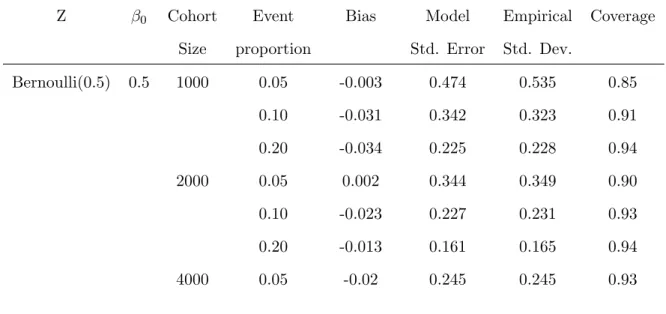
3.1 Summary of Simulation Results of ˆβI for Multiplicative Model · · · 45
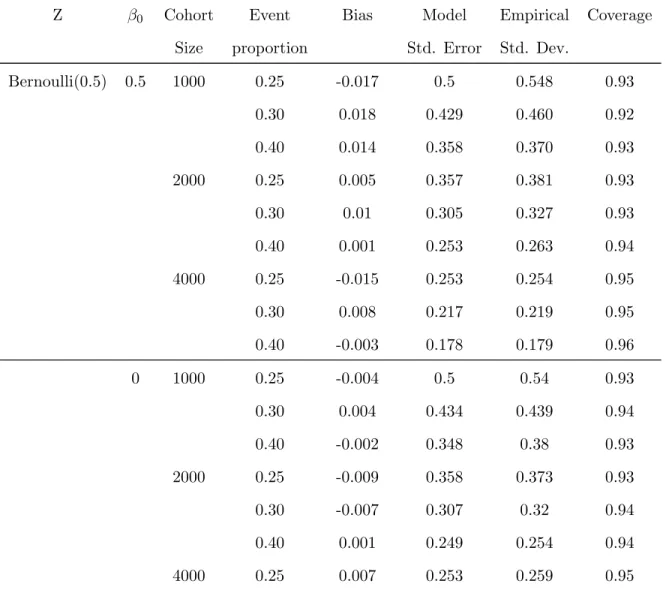
3.2 Summary of Simulation Results of ˆβII for Multiplicative Model · · · 47
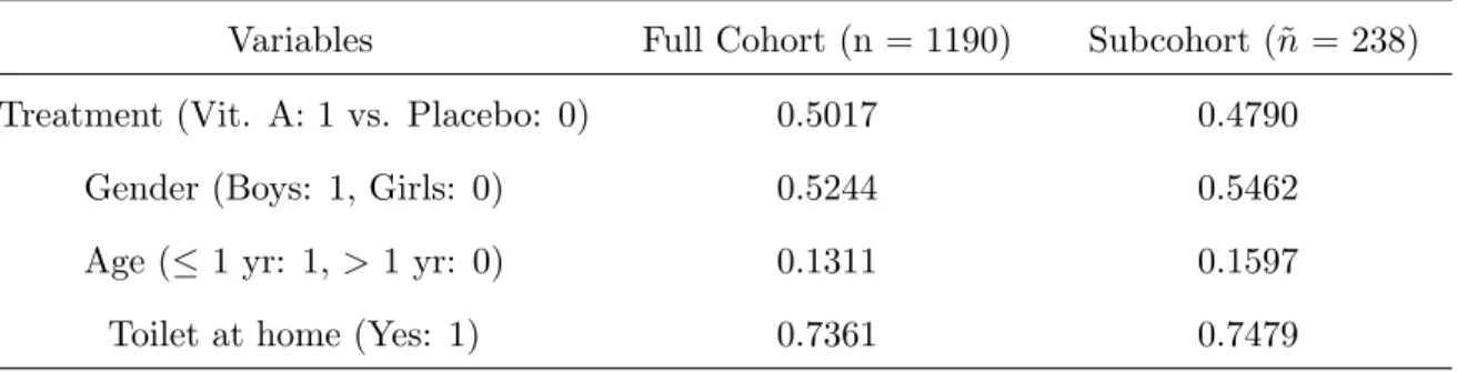
3.3 Baseline Characteristics of the Acute Lower-Respiratory-Tract Infections study · 50 3.4 Estimates and standard errors for the multiplicative rates model with data from case-cohort sample from the ALRI study · · · 50
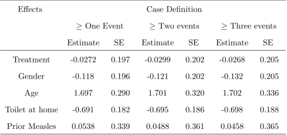
3.5 Estimates and standard errors for different definitions of case for case-cohort sample from the ALRI study · · · 51
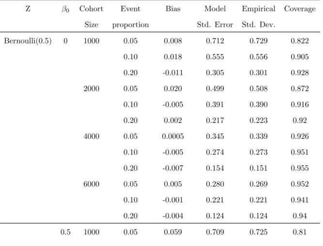
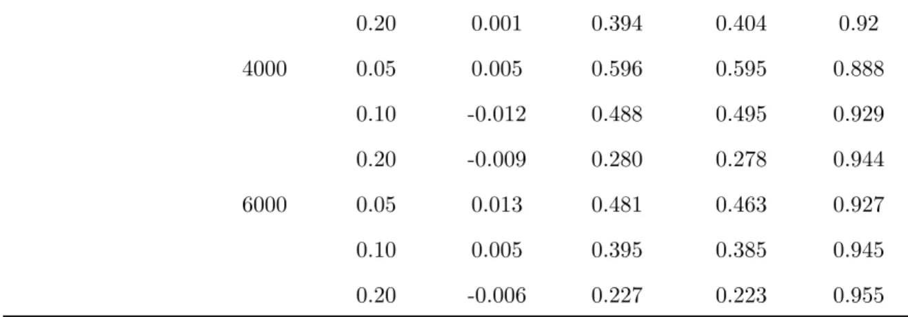
4.1 Summary of Simulation Results of ˆβI for Additive Model · · · 62
4.2 Summary of Simulation Results of ˆβII for Additive Model · · · 64
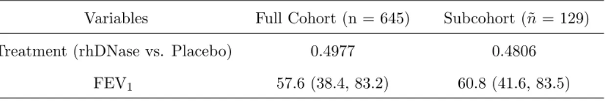
4.3 Baseline Characteristics of the rhDNase study · · · 68
4.4 Estimates and standard errors for the multiplicative rates model with data from GCC sample from the rhDNase study · · · 69
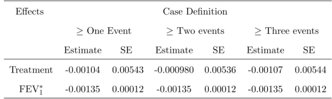
4.5 Estimates and standard errors for different definitions of ‘case’ for GCC sample from the rhDNase study · · · 70
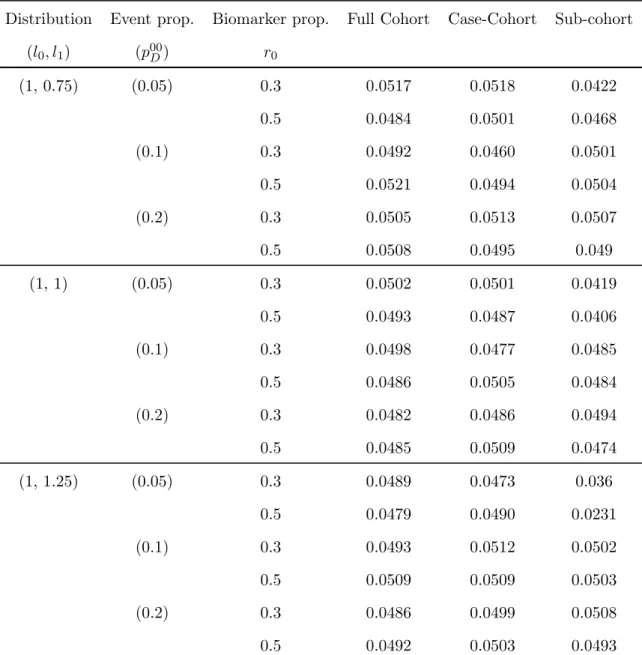
5.1 Summary of Type I Error for Weibull (2) for β1−β0= 0.25 and 1−pC = 0.8) · 80 5.2 Summary of Power Calculation for Exponential Distribution with β1−β0 = 0.5 and 1−pC = 0.7 · · · 82
5.3 Summary of Power Calculation for Exponential Distribution with β1−β0 = 0.5 and 1−pC = 0.8 · · · 83
5.4 Summary of Power Calculation for Exponential Distribution with β1−β0 = 0.5 and 1−pC = 0.9 · · · 84
5.5 Summary of Power Calculation for Weibull(2) Distribution with β1 −β0 = 0.5 and 1−pC = 0.7 · · · 85
5.6 Summary of Power Calculation for Weibull(2) Distribution with β1 −β0 = 0.5 and 1−pC = 0.8 · · · 86
5.7 Summary of Power Calculation for Weibull(2) Distribution with β1 −β0 = 0.5 and 1−pC = 0.9 · · · 87
5.8 Summary of Power Calculation for Weibull(3) Distribution with β1 −β0 = 0.5 and 1−pC = 0.7 · · · 88
5.9 Summary of Power Calculation for Weibull(3) Distribution with β1 −β0 = 0.5 and 1−pC = 0.8 · · · 89
LIST OF FIGURES
CHAPTER 1: INTRODUCTION
Large epidemiologic cohort studies or disease prevention trials are expensive as they re-quire the follow-up of several thousand individuals for a long period of time before producing valuable results (Prentice 1986). The cost mainly arises from the culmination of the raw ma-terials for covariate data ascertainment for all the cohort members. Such raw mama-terials may include blood serum samples, tissue specimens, occupational exposure records, etc. When the disease is rare, much of the covariate data on the disease-free subjects is inessential. Pren-tice (1986) cited the multiple risk factor intervention trial (MRFIT Research Group, 1982), a randomized trial of 12,866 subjects, who were followed-up for an average of seven years and reportedly cost US$100 million. Such studies provide a primary application area for the case-cohort design. In the prevention trial context, a case-cohort design would reduce the cost of assembling the cohort history while allowing for the tracking of the history for the subcohort on an on-going basis.
The case-cohort study design was first proposed by Prentice (1986). It is a retrospective study design nested within a prospective cohort. Specifically, the entire cohort is followed for the disease of interest over time. At a certain time during follow-up, a case-cohort sample is drawn. The case-cohort sample consists of a random sample from the cohort and all subjects who had developed the disease by that time. The expensive or hard to measure covariates are then collected on subjects in the case-cohort sample. Prentice (1986) studied the proportional hazards model for case-cohort data and obtained an estimating equation using pseudo-likelihood approach. In this dissertation, we propose methods to analyze recurrent event data from case-cohort studies.
process of the multivariate counting process. Prentice et al. (1981), Wei et al. (1989), Lawless and Nadeau (1995), Sun et al. (2004), among others considered marginal rates (or mean) model to evaluate the effect of the risk factors on recurrent event data. Some examples include the occurrence of new tumours in patients with superficial bladder cancer (Byar, 1980), recurrent seizures in epileptic patients (Albert 1991), rejection episodes in patients receiving kidney transplants (Cole et al. 1994), repeated infections in HIV-patients (Li and Lagakos 1997) and repeated cardiovascular events in patients (Cui et al. 2008). The two primary frameworks to study the association between the risk factors and the disease recurrence are the additive and multiplicative rates models. Most modern analysis of survival data address multiplicative models for relative risk (rates) using proportional rates models, mostly due to desirable theoretical properties along with the easy interpretation of results (Pepe and Cai 1993, Lawless 1995, Lin et al. 2000, Schaubel et al. 2006, Kang and Cai 2009a). However, researchers may be interested in the risk (rate) difference, rather than the relative measure, attributed to the exposure. Further, the risk difference is more relevant to the public health as it translates directly to the number of disease cases that may be avoided by eliminating the exposure (Kulich and Lin 2000). Consequently, the additive rates models can be considered as an alternative to the multiplicative model (Schaubel et al. 2006, Yin and Cai 2004, Zeng and Cai 2010, Liu et al. 2013, Kang et al. 2013, He et al. 2013).
has not been much work on modeling the marginal rates/mean model for recurrent events under such sampling scheme. Using the intensity model (Andersen and Gill 1982) to analyze recurrent events assumes that all the influence of the prior events on future recurrence is through only the possibly time-varying covariates (Lin et al. 2000). Since, this may not be the case in practice, less restrictive methods need to be developed for such data from case-cohort studies. Motivated by these, we propose statistical methods for modeling recurrent events data from case-cohort studies. We will consider both the multiplicative and additive rates models in analyzing recurrent events data from case-cohort studies.
CHAPTER 2: LITERATURE REVIEW
In this Chapter, we review the literature on the statistical methods for : (i) univariate failure time data arising from case-cohort studies, (ii) correlated failure time data, more specifically, recurrent events from prospective studies and their marginal analysis, (iii) sample size calculation for effects in presence of case-cohort studies when the event is rare. We review the literature on statistical methods for univariate failure time data in Section 2.1, case-cohort studies in Section 2.2, recurrent events analysis from prospective studies in Section 2.3 (including marginal models using multiplicative models and frailty models), additive rates models in Section 2.4, and Power/sample size calculation for case-cohort data in Section 2.5.
2.1 Univariate Failure Time Models
The Cox proportional hazards model (Cox 1972) has been one of the most widely used procedures to study the effects of covariates on failure time. This model assumes that the effect of the covariate on the hazard function is constant over time. A more general version of the Cox model assumes that the hazard function of the failure time, T, associated with the covariates Z, is given by
λ(t|Z(t)) =λ0(t)expβ00Z(t) , (2.1)
where λ0(t) is the unspecified baseline hazard function and β0 is a p-dimensional vector of unknown parameters.
estimated by the partial likelihood score function introduced by (Cox 1975) :
U(β) = n
X
i=1 ˆ τ
0
Zi(t)−
S(1)(β, t) S(0)(β, t)
!
dNi(t), (2.2)
where S(0)(β, t) = n1Pn
j=1Yj(t)exp(βZj(t)) and S(1)(β, t) = 1 n
Pn
j=1Yj(t)Zj(t)exp(βZj(t)). Under some regularity conditions, the maximum partial likelihood estimator, ˆβ, defined as the solution to the score equation, U(β) = 0 converges to a normal distribution as n → ∞ with mean β0 and a variance which can be consistently estimated by −
h
δ
δβ0U(β)|β= ˆβ
i−1
(Andersen and Gill 1982).
2.2 Case-Cohort Studies
Epidemiologic studies are considered to be one of the most reliable methods for assessing the variation in rate of mortality and to study the effect of covariates on the rate in the population. When the event of interest is rare or the relationship that is of interest is complex, cohort studies would require large number of subjects and/or long periods of follow-up in order to accumulate enough failures to have sufficient statistical power to make meaningful conclusions. However, this would increase the cost of collecting such covariate information on all subjects, if feasible. Prentice (1986) proposed the case-cohort design to reduce the number of subjects for whom the covariate information is collected, hence reducing the overall cost. This method involves the selection of a random sample from the entire cohort, which is called the cohort and the assembly of the covariate information on the individuals in this sub-cohort as well as the subjects who experienced the event of interest during the follow-up period. The sub-cohort also provides a basis for monitoring the covariates during the follow-up of the cohort. Studying the relative risk process is quite natural in understanding the effect of the covariate history on the event rates. Based on the relative risk regression model (Cox 1972), the hazard function of the i-th subject, at time t, is modeled by
where r(.) is a known function with r(0) = 1. The pseudo-likelihood function for the estima-tion ofβ0 has the form :
˜ L(β0) =
n
Y
i=1
rii
X
l∈R(ti)˜ rli
∆i
, (2.4)
where ˜R(t) = D(t)∪ Sc, Sc is the set of all individuals in the sub-cohort, D(t) is the set of all individuals who have observed a failure at time t. It can be written as D(t) = {i|Ni(t)6=Ni(t−)} and rli = Yl(ti)r{β0Zl(ti)}. Covariate information is assumed to be available only for the set, K(t)∪Sc at time t, where K(t) ={i|Ni(t) = 1}. The maximum pseudo-likelihood estimate, ˆβP L is defined by ˜U( ˆβP L) = 0 where ˜U(β) is defined as
˜
U(β) = δ
δβ0logL(β) =˜
n
X
i=1 ˜ U(β) =
n
X
i=1 ∆i
cii−
X
l∈R(ti)˜ bli
X
l∈R(ti)˜ rli
, (2.5)
wherebli =Yl(ti)Zl(ti)r{β0Zl(ti)}; cii=biir0{β0Zi(ti)} and r0(t) = δβδ0r(t). Prentice (1986)
showed that the variance of n−1/2U(β0) is given by
˜
V(β) =I(β) + 2 n
X
i=1
∆i∆(t˜ i)
X
k|tk<ti ∆kvki,
whereI(β) =− δ
δβ0U(β), vki=−Pj∈R(ti)˜
B
k+bik−bjk Rk+rik−rjk
0
cji−BiRi
rjiRi−1, Ri =Pk∈R(ti)˜ rki, Bi =Pk∈R(ti)˜ bki and ˜∆(t) = 1 if ˜R(t) 6= Sc, 0, o.w. Hence, by Taylor series expansion, we have the variance ofn1/2βˆP L−β0
is given byI(β0)−1V˜(β0)I(β0)−1. A natural estimator of the cumulative baseline rate is proposed as
ˆ
Λ0(t) = ˜nn−1 ˆ t
0
X
l∈Sc Yl(u)r
n
ˆ
βP L0 Zl(u)
o
−1
dN¯(u),
where ¯N(t) =Pn
Self and Prentice (1988) developed the asymptotic distribution theory for the case-cohort maximum pseudo-likelihood estimator and related quantities, with slightly different pseu-dolikelihood and variance estimator from the ones proposed by Prentice (1986). In their formulation of the risk set, only the sub-cohort individuals were considered, whereas in the original Prentice (1986) paper, the risk set included a non-subcohort individual that fails at a particular time point. In Self and Prentice (1988), they considered a similar relative risk regression model as (2.3). The maximum pseudolikelihood estimator, ˆβsp, is defined as the solution to U(β) = δβδ0logL(β) = 0, where we have˜
logL(β) =˜ X i∈C
ˆ τ 0
logrβ0Zi(t) dNi(t)− ˆ τ
0 log
X
j∈Sc
Yj(t)r β0Zj(t)
dNi(t),
(2.6) where C is the cohort and Sc is the subcohort of size ˜n. Under some regularity conditions, they proved that ˆβspconverges in probability toβ0andn−1/2U(β0) converges to a Normal dis-tribution with mean zero and variance Σ(β0)+∆(β0), where Σ(β) =−limn→∞n1 ∂
2
∂β∂β0logL(β)˜
and ∆(β) consists of the contributions of the covariance among the components induced by the random sampling and have a complicated expression. Hence, by the Taylor series expan-sion,n1/2
ˆ βsp−β0
converges to a Gaussian distribution with mean 0 and covariance matrix Σ(β0)−1+ Σ(β0)−1∆(β0)Σ(β0)−1. Self & Prentice (1988), in their paper, propose consistent estimators for Σ(β0) and ∆(β0). For the cumulative hazard function, Λ0(t), the proposed estimator is given by
Λ0(t) = ˜nn−1 ˆ t
0
X
l∈Sc Yl(u)r
n
ˆ βsp0 Zl(u)
o
−1
dN¯(u). (2.7)
n1/2βˆsp−β0
andn1/2Λ˜0(t)−Λ0(t)
different from the one proposed by Self and Prentice (1988) but it has been shown to converge to Σ(β0)−1+ Σ(β0)−1∆(β0)Σ(β0)−1.
The variance estimators proposed in these two papers (Prentice 1986, Self and Pren-tice 1988) are quite complicated. There have been many methods proposed to estimate the variance of the estimators from the pseudo-likelihood. Wacholder et al. (1989) proposed a bootstrap estimate of the variance of the covariate effect estimator. Their method echoes the original case-cohort sampling scheme by resampling cases and sub-cohort controls separately. This method is quite intensive computationally and would be quite time-consuming for large studies but it avoids the direct computation of the covariance among score components.
Barlow (1994) proposed a robust estimator of the variance based on the influence of an individual observation on the overall score. In the paper, the author assumed the standard Cox Proportional Hazard regression model for the relative risk as seen in equation (2.3). The conditional probability of failure at timetj is given by
pi(tj) =
Yi(tj)wi(tj)ri(tj)
Pn
k=1Yk(tj)wk(tj)rk(tj) ,
where the weight of the i-th subject at timetis given by
wi(t) =
1 ifdNi(t) = 1, m(t)
˜
m(t) ifdNi(t) = 0 andi∈Sc, 0 ifdNi(t) = 0 and i6∈Sc
wherem(t) is the number of disease-free individuals in the full-cohort who are at risk at time tand ˜m(t) is the number of disease-free individuals in the random sub-cohort who are at risk at time t; ri(t) = exp{β00Zi(t)}. One can easily note that Prentice (1986) used the weights as binary indicator, it being = 1 for the i-th individual at time t if dNi(t) = 1 or i ∈Sc and zero, otherwise. The Self & Prentice method used only the denominator summed over the subcohort members in the likelihood. The estimation of the unknown parameter follows directly from the log-likelihood of the conditional probability, i.e.,Pn
i=1 ´τ
P
t
Pn
i=1dNi(t)log(pi(t)). The robust variance estimator that was proposed in the paper, using the infinitesimal jackknife estimator, is given by ˆV( ˜β) = 1nPn
i=1eiˆˆe
0
i where ˆei = ˜β − ˜
β−(i) = I−1( ˜β)ˆci(t0), ci(t0) is defined as the influence of an observation on the overall score for a particular individual i at time t0 and ˆei is the change in ˜β if the i-th observation is deleted. Further,ci(t0) is given by
ci(t0) = ˆ t0
0
Yi(t) [dNi(t)−λi(t)] (Zi(t)−EZ(t))dN¯(t),
where EZ(t) = Pni=1pi(t)Zi(t). I( ˜β) is the information matrix generated by the pseudo-likelihood function. We can estimateci(t0) by ˆci(t0) =
´t0
0 Yi(t) [dNi(t)−pˆi(t)]
Zi(t)−EˆZ(t)
×dN¯(t) and I( ˜β) =P
t
P
ipˆi(t)
h
zi(t)−E(t)ˆ
i h
zi(t)−E(t)ˆ
i0
.
Lin and Ying (1993) tackled the problem of missing covariate data under Cox Propor-tional Hazards regression model, of which the case-cohort design was a special case. They proposed an approximated partial-likelihood score function for the estimation of the regres-sion parameters. A new variance-covariance estimator which is much easier to calculate than that Prentice (1986) and Self and Prentice (1988) was also proposed. The standard Cox PH regression model was assumed, as given in equation (2.1). Suppose that the data consist of iid random quintuplets (Xi,∆i, Zi(.), H0i(.),Hi(.)) where Zi(.) ={Zi1(.), Zi2(.), . . . , Z1p(.)}0 may not be fully observed andH0i(.) is an indicator function andHi(.) is ap×pmatrix with the indicator functionsH1i(.), H2i(.), . . . , Hpi(.) being the diagonal elements. Considering the original case-cohort design, we haveHi(.) =Ipwhich is thep×pidentity matrix andH0i(.) is 1 if the i-th subject belongs to the sub-cohort and zero, otherwise. The approximate partial likelihood score function can be written as
˜
UH(β) = n
X
i=1
∆iHi(Xi){Zi(Xi)−EH(β, Xi)},
where EH(β, Xi) =
S(1)H (β,Xi) S(0)H (β,Xi); S
(d)
H (β, t) = 1n
Pn
i=1H0i(t)Yi(t)exp{β
0Zi(t)}Zi(t)⊗d. Let us define the root of the estimating equation, ˜UH(β) = 0, by ˜βH. Under certain regularity conditions, n1/2
˜ βH −β0
with mean zero and variance given byA−1(β0)V(β0)A−1(β0), where An(β) =−1 n
δ
δβ0U˜H(β), limn→∞An(β) =A(β),V(β) =E W1(β)⊗2
,
Wi(β) = ∆iHi(Xi){Zi(Xi)−eH(β, Xi)}− ˆ Xi
0
h(t)
h0(t)H0i(t){Zi(t)−eH(β, t)}exp(β
0Z
i(t))dΛ0(t),
where eH(β, t) =
s(1)H (β,t) s(0)H (β,t), s
(d)
H (β, t) = E(S (d)
H (β, t)) for d = 0, 1; h(t) = E(Hi(t)), hk(t) = E(Hki(t)) for all k= 0,1, . . . , p. Therefore, The covariance matrix can be approximated by An−1( ˜βH) ˆV( ˜βH)An−1( ˜βH) where ˆV(β) = n1Pn
i=1Wi(β)ˆ
⊗2 and
ˆ
Wi(β) = ∆iHi(Xi){Zi(Xi)−EH(β, Xi)}
−1 n
n
X
l=1
∆lYi(Xl)H0i(Xl)Hl(Xl)exp{β0Zi(Xl)} ×(Zi(Xl)−EH(β, Xl)) SH(0)(β, Xl)
.
For the case-cohort design, the variance estimatorA−n1( ˜βH) ˆV( ˜βH)A−n1( ˜βH) is much easier to calculate, even when we have time-dependent covariates, than Prentice (1986) and Self and Prentice (1988). Another advantage of the proposed method is that incomplete covariate information on the covariates is allowed. Furthermore, the form of the proposed estimator remains unchanged under multiple sub-cohort augmentations. A natural estimator of the cumulative hazard function is proposed as
˜
Λ( ˜βH, t) = n
X
i=1
I(Xi6t)H0i(Xi)∆i nSH(0)( ˜βH, Xi)
= ˆ t
0
H0i(u)dNi(u)
nSH(0)( ˜βH, u) .
The processn1/2Λ( ˜˜ βH, t)−Λ0(t)
converges weakly to a Gaussian process with mean zero and covariance function
ψ(t, s) = ˆ t∧s
0
dΛ0(u) s(0)(β
0, u)
+J0(t)A−1(β0)V(β0)A−1(β0)0J(s)−J0(s)A−1(β0)G(t)−J0(t)A−1(β0)G(s), (2.8) whereJ(t) =´0ts(1)(β0,u)dΛ0(u)
s(0)(β
0,u) and G(t) =E[
´∞
0 ´t∧v
0
H0i(u)exp{β00Zi(u)}dΛ0(u)
s(0)(β
0,u)
×Hi(v)−Hh00i(v)(v) h(v)
that this might not be the best choice ifH0i(Xi) = 0 for most of the non-zero ∆i’s. Hence, for the original case-cohort design, the authors recommend to use the formula proposed by Self and Prentice (1988) as seen in equation (2.7) rather than this.
Chen and Lo (1999) proposed a class of estimating equations for case-cohort design based on the partial likelihood score function, which lead to simple estimators that improve Pren-tice’s pseudolikelihood estimator. The authors explored the usual Cox PH model (2.3), with r(.) being replaced by exp(.) and did not include any time-dependent covariates. They observed the triplets (Xi,∆i, Zi) for the i-th individual. One can note that
E(Z |X=t,∆ = 1) =
EZeβ0ZI(X>t) E(eβ0Z
I(X>t)) =
pEZeβ0ZI(X >t)|∆ = 1+ (1−p)EZeβ0ZI(X >t)|∆ = 0 pE(eβ0Z
I(X>t)|∆ = 1) + (1−p)E(eβ0Z
I(X>t)|∆ = 0) , (2.9)
where p = P(∆ = 1). Let F1 and F0 be the conditional joint distributions of (X, Y) given ∆ = 1 and ∆ = 0 respectively. Further, suppose thatR1 is the index set of random sample of k1 cases and R0 is the index set of random sample of k0 censored individuals. Then, one can estimate Fl, l = 0, 1 by the respective empirical counterpart, Rl. Hence, replacing the population quantities by the empirical analogues, the authors proposed the following estimating function :
U(β) = X i∈R1
ˆ ∞
0
"
Zi−
(ˆp/k1)P
j∈R1
tZje
β0Zi+{(1−p)/k0ˆ }P
j∈R0
t Zje β0Zi (ˆp/k1)P
j∈R1
t e β0Zi
+{(1−p)/k0ˆ }P
j∈R0
t e β0Zi
#
dNi(t). (2.10)
The authors considered several cases with different estimates of p depending on how much information one has about the data and considered the consistent estimator of the unknown parameters, β0, and the corresponding covariance terms for the asymptotic distribution of n1/2
ˆ
βCL−β0
reduces to
U(β) = n
X
i=1 ˆ ∞
0
"
Zi−
P
j∈R1
t Zje
β0Zi + (n0/n∗
0)
P
j∈R0
t Zje β0Zi
P
j∈R1
te β0Zi
+ (n0/n∗0)P
j∈R0
t e β0Zi
#
dNi(t) = 0. (2.11)
The solution to this equation, ˆβcl, is consistent for β0 and n1/2
ˆ βcl−β0
converges to a Gaussian distribution with mean zero and variance given by
σ2 = 1 nΣ
−1 1 +
1 n∗0 −
1 n
Σ−11
Σ−01−pV1−1−p p E
⊗2 0
Σ−11,
where Σ1 = var(W∗), Σ0 = var(W), V1 = var(W | ∆ = 1), E0 = E(W | ∆ = 0), W∗ = {Z −m(Y)}∆, W = ´0∞{Z −m(t)}eβZI(Y > t)dΛ
0(t), m(t) = E(Z | Y = t,∆ = 1). Kulich and Lin (2000) demonstrated the use of case-cohort data in estimating the regression parameter of an additive hazards regression model, where the conditional hazard function given a set of the covariates is the sum of an arbitrary baseline hazard and a function of the unknown regression parameter and the covariates. We have discussed this in details when discussing the literature for additive rates models.
Chen (2001) proposed a more efficient estimator by using local averages type of weights. The paper focuses on a unified approach for the parameter estimation of Cox PH model under different cohort sampling schemes, like nested case control, case-cohort and classical case-cohort methods. The sample reuse approach proposed via local averaging leads to more efficient estimators and this method is applicable to more complex sampling designs. The estimating equation they propose is the following :
U(β) = n
X
i=1 ˆ ∞
0
[hi(t)−
Pn
j=1W
∗
j(t)hj(t)exp(β
0Zj(t))Yj(t)
Pn
j=1W
∗
j(t)exp(β0Zj(t))Yj(t)
]Wi∗(t)dNi(t) = 0, (2.12)
δj =1(j-th individual is sampled), n0 & n∗0 is the number of censored individuals in the co-hort and the subcoco-hort, respectively. Chen (2001) proposed the following weight function, Wj∗(t) =Wj∗=δj/rn(Xj, δj), where Xj =Tj ∧Cj (when we have only one event) and
rn(t, d) =
Pn
l=1δl∆l1(xl∈[ti−1, ti])
Pn
l=1δl1(xl∈[ti−1, ti])
if d =1 and t∈[ti−1, ti] =
Pn
l=1(1−δl)∆l1(xl∈[sj−1, sj])
Pn
l=1(1−δl)1(xl∈[sj−1, sj])
if d =0 and t∈[sj−1, sj],
where 0 = t0 ≤ t1 ≤ . . . ≤ tan = τ and 0 = s0 ≤ s1 ≤ . . . ≤ sbn = τ are two partitions which satisfy certain conditions, resulting in more efficient estimation of the parameters. The author noted that the existing work on case-cohort sampling on survival analysis is highly dependent on the specific sampling design and the methods result in inefficient estimates of the regression parameters. Under the regularity conditions, the solution to equation (2.12), ˆβh, is consistent forβ0 and the asymptotic distribution ofn1/2
ˆ βh−β0
is Gaussian with mean zero and variance Σ−h,Z1 (Σh,h+ Σ∗h) Σ
−1
h,Z with Σh,Z = cov(M˜h, MZ˜), Σh,h = cov(M˜h, M˜h), Σ∗hcov(W˜h, M˜h),Mh=
´τ
0 h(t)dM(t),W˜h= (1/π−1)(M˜h−Mh˜o),M˜ho =E(M˜h |Y,∆), ˜h(t) = h(t)−E(h(t)). Kulich and Lin (2004) developed a class of weighted estimating equations with time-dependent weight functions for stratified case-cohort designs. The authors in this paper considered the Cox (1972) regression model as described in (2.3) with exp(.) as the function r(.). They considered a cohort of n subjects who can be divided into K mutually exclusive strata based on a discrete random variable V. They assumed that V affects the failure time only through the covariates, i.e., T is independent of V given Z(.). The data observed is the following : (Xki = Tki∧Cki,∆ki, Zki(t),0 6 t 6 τ, Vki, ξki) for the individuals in the sub-cohort and (Xki,∆ki, Zki(Xki)) for all the cases outside the sub-cohort. The estimating equation is given by
U(β) = K
X
k=1 nk
X
i=1 ˆ τ
0
[Zki(t)−EC(β, t)]dNki(t) = 0, (2.13)
where EC(β, t) =
S(1)C (β,t) S(0)C (β,t), S
(d)
C (β, t) =
PK k=1
Pnk
i=1%ki(t)Zki(t)Yki(t)eβ
0
Zki(t)
PK k=1
Pnk
i=1%ki(t)Yki(t)eβ
is the indicator that the individual is included in the sub-cohort and ˆαk(.) is a function of the controls (because of the separation between the cases and the controls). The authors proposed a doubly weighted estimator
ˆ αk(t) =
(nk X
i=1
(1−∆ki)Aki(t)
)−1(nk X
i=1
ξki(1−∆ki)Aki(t)
)
,
whereAki(t) is a diagonal matrix with m potentially different random processes on the diag-onal. Redefine the at-risk covariate average asEDW(β, t) ={SDW(0) (β, t)}−1S
(1)
DW(β, t) where SDW(1) (β, t) and SDW(0) (β, t) are the matrix counterparts of SC(1)(β, t) and SC(0)(β, t), respec-tively. Based on these, the authors showed that, under certain regularity conditions, ˆβDW is a consistent estimator ofβ0 and n1/2
ˆ
βDW −β0
converges to a Gaussian distribution with mean 0 and varianceI−F1+IF−1ΣDWI−F1, whereIF =
´τ 0
h
s(2)(β,t)
s(0)(β,t)−e(β, t)
⊗2is(0)(β, t)dΛ0(t), s(d)(β, t) =E(Zi(t)Yi(t)eβ0Zi(t)), d = 0,1,2; e(β, t) = ss(1)(0)(β,t)(β,t), ΣDW =
PK
k=1qk 1−αk
αk Ek
(1−∆i) ´τ
0 Rki(t)−µ
−1
k (t)Aki(t)ψk(t)
dΛ0(t)
⊗2
with qk = P(V = k), αk = P(ξ = 1 | V = k), Rki(t) = (Zki(t)−e(β, t))eβ
0Z
ki(t)Y
ki(t), µk = E[(1−∆ki)Aki(t)] and ψk(t) = E[(1−∆ki)Rki(t)].
Nan (2004) developed semi-parametric efficient estimators, obtained by solving the the efficient score equation with the help of the Newton-Raphson algorithm. Lu and Tsiatis (2006) proposed a general class of semi-parametric transformation model. They considered weighted estimating equations for simultaneous estimation of the regression parameters and the transformation function. The semi-parametric linear transformation model is specified by
H(T) =−β00Z+,
distribution, independent of the censoring process and covariates. The corresponding esti-mating equations are given by
n
X
i=1 πi
dNi(t)−Yi(t)dΛ{H(t) +β0Zi}
= 0 (t>0), H(0) =−∞,
n
X
i=1 ˆ ∞
0
ZiπidNi(t)−Yi(t)dΛ{H(t) +β0Zi}
= 0.
The authors showed that the resulting regression estimators are asymptotically normal, with a closed form variance-covariance matrix that can be consistently estimated by the usual plug-in estimators. Lu and Shih (2006) extended the case-cohort design to clustered data, where each clustered comprises of correlated individuals, whose structure of dependence is kept unspecified. The estimating equation is defined as
U(β) = n
X
i=1 m
X
j=1
Zij(Xij)−E(β, Xij¯ )δij,
where ¯E(β, t) = SS¯¯10(β,t)(β,t), ¯S
d(β, t) = Pn
i=1
Pm
j ∆ijYij(t)eβ
0Zij(t)
Zij(t)⊗d, ∆ij is an individual indicator that equals 1 if individual (i, j) is selected for the subcohort, and 0, otherwise and δij is the indicator of whether the j-th individual in the i-th cluster observes the event or is censored. Kang and Cai (2009a) considered marginal hazards model for case-cohort data with multiple disease outcomes. Time to different events are modeled simultaneously in order to compare the effect of a risk factor on different types of diseases. They have proposed valid statistical methods that take the correlations among the outcomes from the same subject into account. They have considered the multiplicative intensity process model, which is specified by
λik(t|Zik(t)) =Yik(t)λ0k(t)eβ
0
0Zik(t),
(2011) developed estimating equation for clustered failure time data assuming a marginal haz-ards model, with a common baseline hazard and common regression coefficient across clusters. One of the key advantages of the case-cohort design is its ability to use the same sub-cohort for several diseases or for sub-types of diseases (Prentice 1986, Wacholder et al. 1989, Langholz and Thomas 1990, Wacholder 1991). The availability of the case-cohort sub-cohort may be useful for study monitoring and can be considered to be a natural comparison group at all disease occurrence times for all of the different diseases. Chen and Chen (2014) extended the case-cohort design to recurrent events with specific clustering feature using a modified Cox-type self- exciting intensity model. Under this model, conditional on the covariates and history of events upto time t, the intensity function of N(.) (simple point process) is given by
λ(t) =µ(t)exp{Ψ(t, θ)},
where Ψ(t, θ) = β0Z(t) +φ(t), µ(t) is the unspecified baseline intensity, Z(t) is the time-varying p-dimensional vector of covariate, β is the vector of regression coefficients, φ(t) is a self-exciting term depending on past events of the process and θ is the combined finite dimensional parameters to be specified. The pseudo-likelihood score equation for θ is given by
log L(θ) = n
X
i=1 ˆ Ci
0
"
ψi(t, θ)−
Pn
j=1jψj(t, θ)Yj(t)exp{Ψj(t)}
Pn
j=1jYj(t)exp{Ψj(t)}
#
dNi(t) = 0, (2.14)
where ψ(t, θ) = ∂θ∂ Ψ(t, θ). The authors went onto show the asymptotic properties of the solution to the above equation, under certain regularity conditions.
2.3 Recurrent Events Data
infections in HIV-patients (Li and Lagakos 1997), repeated cardiovascular events in patients (Cui et al. 2008). In this section, we look at the different ways one can model the recurrent event data and the assumptions that are attached to it. In the following subsections, we will summarize the marginal models (more specifically, intensity models and rate & mean mod-els) which do not assume anything about the nature of the dependence among the recurrent events and the frailty model which explicitly specifies the relationship among the repeated events.
2.3.1 Marginal Models using Multiplicative Models
Prentice et al. (1981) considered two stratified proportional hazards type of regression models for modeling the intensity function in terms of the covariates and the failure time history. The main diference between the two models is that one of them specifies the baseline intensity function as a function of time from the beginning of study, while the other specifies it as a function of time from the subject’s immediately preceding failure. LetZ(t) ={z(u)| u 6 t} be the covariate process upto time t and N(t) = {n(u) | u 6 t}, where n(u) is the number of failures on a study subject prior to time t. The counting process N(t) is equivalent to random failure time, T1, T2, . . . , Tn(t) in [0, t). The authors define the hazard or the intensity function at time t as the instantaneous rate of failure at time t given the covariate and counting process.
λ{t|N(t), Z(t)}= lim δt→0
P(t6Tn(t)+16t+δt|N(t), Z(t)) δt
⇒λ{t|N(t), Z(t)}=λ0s(t)eβ0sz(t), time from the beginning of study (2.15)
or λ{t|N(t), Z(t)}=λ0s(t−tn(t))eβ0sz(t), time from the immediately preceeding failure, (2.16)
where they studied the time from the beginning of the study is given by
L(β0) =Y s>1
ds
Y
i=1
exp[β00zsi(tsi)]
P
l∈R(tsi,s)exp[β00zl(tsi)] ,
whereR(t, s) is the risk set at timetfor the s-th stratum. For the time from the last observed failure, we have
L(β0) =Y s>1
ds
Y
i=1
exp[β00zsi(tsi)]
P
l∈R˜(usi,s)exp[β00ztl+u+si(tsi)] ,
where ˜R(t, s) is the risk set at gap-time t stratum-s. tl is the last failure time on subject l prior to entry into stratum s. The authors note that ordinary asymptotic likelihood methods can be applied to both the likelihood functions (Cox 1975) though consideration should be given to the size and to the number of failures in each stratum. Andersen and Gill (1982) explored the Cox PH regression model (as in equation (2.1)). The authors extended the Cox PH model for a single failure time data where the effect of the covariate is proportional on the hazard, to the multivariate counting process, where the effect of the covariate process is proportional on the intensity function. They showed that Mi(t) = Ni(t)−´0tdΛi(t) are local square-integrable martingales on the time interval [0, 1]. The solution to the estimating equation U(β) = 0 is denoted by ˆβ, whereU(β) is defined as in (2.2), withYi(t) defined as an indicator function showing whether the individual is still under observation or not. They showed that ˆβ is consistent forβ0 and n−1/2U(β0) converges to a Gaussian distribution with mean zero and variance, Σ(β0), where Σ(β) =
´1 0
s(2)(β,t)
s(0)(β,t) −
s(1)(β,t)
s(0)(β,t)
⊗2
s(0)(β, t)λ0(t)dt. Wei et al. (1989) noted that many survival studies record the times to two or more failures per subject, where the failure types might be completely different or they may be repetitions of the same type. The authors proposed to model the marginal distribution of each failure time variable with a Cox-type PH regression model. In this approach, no structure is imposed on the dependence of the different failure times for each subject. The hazard function for the k-th type of failure time of the i-th subject is given by
The k-th failure-specific partial likelihood (Cox, 1975) is defined as
Lk(β0) = n
Y
i=1
exp[β00Zki(Xki)]
P
l∈R(Xki)exp[β
0
0Zli(Xki)] ,
whereR(t) ={i:Xki >t}is the set of individuals who are at risk of observing the k-th type of failure just prior to time t. Under certain regularity conditions, the solution to the partial likelihood equation, ∂Lk(β)∂β = 0, given by ˆβk, will be consistent for the unknown parameter, βk0. n1/2( ˆβ−β0) = n1/2( ˆβ1 −β01,β2ˆ −β02, . . . ,βKˆ −β0K) converges asymptotically to a Normal distribution with zero-mean and variance Q with elements equal to Dij( ˆβi,βj), i,ˆ j = 1,2, . . . , K and Dij( ˆβi,βˆj) can be consistently estimated by ˆAi( ˆβi)−1Bˆ( ˆβi,βˆj) ˆAj( ˆβj)−1 with ˆAi(βi)−1 = 1nPk∆ik
hS(2)(βi,X
ik) S(0)(βi,Xik) −(
S(1)(βi,X
ik) S(0)(βi,Xik))
⊗2i, ˆB( ˆβ
i,βˆj) = 1nPkWik( ˆβi)Wjk( ˆβj)0, Wik(βk) =
∆ik−Pnm=1
∆imYik(Xim)eβkZik0 (Xim) S(0)(βi,X
ik)
×hZik(Xim)−S
(1)(βi,Xik)
S(0)(βi,X
ik)
i
, S(d)(β, t) = 1nPn
i=1Zi(t)Yi(t)eβ
0Zi(t)
.
Pepe and Cai (1993) looked at different methods to display and analyze multiple failure time data. The authors looked at the rate function. They defined the rate functions as rF(t) = lim∆→0∆1P[event occurred in (t, t+ ∆)|at risk and no event observed att] (rate of first infection) and rR(t) =
lim∆→0∆1P[event occurred in (t, t+ ∆)| at risk and event previously observed att] (rate of recurrent infection). Suppose that rF and rR are functions of time that involve certain parameters,α and γ asrαF andrRγ respectively. The likelihood for α is given by
L(α) = Y ti∈D
rαF(ti)exp
− ˆ ti
0
rαF(u)du
×
Y
tj∈D
rαF(tj)exp{− ˆ tj
0
rαF(u)du}
,
where D is the set of times when the event occurred for the first time; O is the set of observation times for subjects censored or lost to follow-up due to competing risk events. The corresponding score function is given by
SF(α) = ˆ
fα(t)
where fα(t) = ∂logrαF(t) ∂α , N
F(t) = the number of individuals who had the event observed by time t, andYF(t) = the number of individuals under observation and who had not observed any prior event at t. By definition, E dNF(t)/YF(t)|YF(t)=rFα(t)dt. The authors note that under mild regularity conditions, the solution to the estimating equation (2.18) should be a consistent estimator of α, even when fα(t) is somewhat different from ∂logr
F α(t)
∂α . They further noted that setting fα(t) at this quantity would yield the most efficient estimator. The authors also observed that likelihood-based estimation ofrRγ would require specifying a model for the joint distribution of recurrence times within the same individual, but one can get consistent estimates ofγ from an estimating equation like (2.18).
SR(α) = n
X
i=1
SiR(α) = n
X
i=1 ˆ
Iγ(t)
dNiR(t)−YiR(t)rRα(t)dt = 0, (2.19)
whereNiR(t) is the number of events observed by timetfor the i-th individual with previously observed events, YiR(t) is the indicator that the i-th individual, with previously observed events, is at-risk of an event at t, and Iγ(t) is some bounded deterministic vector-valued function whose dimension is the same as the dimension of γ. The authors showed that the solution to the estimating equation (2.19), ˆγ, is consistent estimator ofγ and n−1/2SR(t)−D→ N(O, V(t)), where V(t) is the variance- covariance matrix for SiR(t) and one can get the asymptotic distribution of ˆγ from Taylor series expansion.
Lawless and Nadeau (1995) presented non-parametric methods and regression models to estimate the cumulative mean function (CMF), defined asM(t) =E(Ni(t)), whereNi(t) is the number of events occurring in time [0, t]. The main objective is to estimateM(t) based on the observed times times, which are defined asti1 6ti2 6. . .6tiri for the i-th individual over the interval [0,τi] (i = 1,2,. . ., k) and the individuals are independent. For simplicity, the authors presented the results in a discrete-time framework. Defineδi(t) = 1, ift6τi, 0 o.w., to denote whether an individual observed an event. Further, letni(t)>0 denote the number of events that occur at time ‘t’ for the i-th individual so thatm(t) =E{ni(t)}andM(t) =Pt
s=0m(s). The maximum likelihood estimator the authors proposed is given by ˆM(t) =Pt
s=0 n.(s) δ.(s),06 t6τ = maxi(τi), wheren.(t) =
Pk
i=1δi(t)ni(t) andδ.(t) =
Pk
the variance of ˆM(t) asvar( ˆM(t)) =Pk
i=1
Pt
s=0
Pt
u=0
δi(s)δi(u)
δ.(s)δ.(u)cov(ni(s), ni(u)). The authors further extended the idea to develop similar approach for a flexible family of regression models. The following regression model
E(ni(t)) =mi(t) =m0(t)Pi(t)g(zi(t), β0)
was considered, whereβ0 is a p-dimensional vector of regression parameters, g is a positive valued function, m0(t)>0 is the baseline mean function and Pi(t) is some known function. Noting that m0(t) = R(t,βn.(t)0) and R(t, β0) =
Pk
i=1δi(t)gi(t), the estimating equation for β is given by Pk
j=1
P
l∈Dj
n∂loggl(tj)
∂β −
∂R(tj,β) ∂β
o
= 0, where Dj represents the set of individuals with events attj, including repetitions for an individual at that time. Under mild conditions, the solution to this estimating equation, ˆβ, is consistent for β0. Defining
Wi(β, s) =
∂loggi(s) ∂β −
∂logR(s, β) ∂β ,
ˆ B1i(t) =
t
X
s=0
δi(s)Wi( ˆβ, s)[ni(s)−gˆi(s) ˆm0(s)],
where ˆgi(s) =Pi(s)g(xi,β), ˆˆ B1 = 1kPki=1Bˆ1iBˆ1i0 and ˆA1 = 1kPki=1
Pτ
s=0δi(s) ˆm0(s)∂ˆgi(s)∂βˆ ×Wi( ˆβ, s)0, we have k1/2βˆ−β0
converges asymptotically to a Gaussian distribution with mean 0 and a sandwich variance term var( ˆˆ β) = ˆA−11Bˆ1( ˆA−11)0. Lawless (1995) discussed different ways of introducing covariates in the analysis of recurrent events and the distinction between rate (and mean) function and intensity functions event process characterizations. The author defines the rate of occurrence function is r(t) = ∂E(N∂t(t)) and the mean function is given by
E[N(t)] = ˆ t
0
r(u)du (2.20)
Renewal type of models based on intervals between successive events would be characterized by
λ(t;Hit, zi) =hj(t−tij)exp(βjzi),
whereNi(t−) =j (Gail et al. 1980) specifies that for each subject the times to the first event and between successive events are independent random variables and they do not necessarily have the same distribution;Ht={N(s)|s < t}is the history of the process up to time t;tij is the j-th observed event time for the i-th individual and βj are the regression parameters. The authors used Lawless and Nadeau’s (1995) approach to estimate β, yielding R0(t) = ´t
0
dN(u)
Pn
i=1δi(u)φi(zi,β) andN(u) is the total number of events observed at u. The authors further
proposed the joint distribution ofn1/2
ˆ
β−β,R0(t)ˆ −R0(t)
. They noted that the marginal analyses for means are quite easy to interpret and may be made robust to other assumptions about the recurrent event process, provided that the observation period [0, τi] for the i-th individual (for all i) are independent of the corresponding event process.
Cook et al. (1996) investigated robust non-parametric tests, in the sense, that these meth-ods do not rely on distributional assumptions of the event-generating process, for recurrent event data. They have further explored a family of generalized pseudo-score statistics (Lawless and Nadeau 1995) in which weight functions may be chosen to generate tests sensitive to var-ious types of departure from the null hypothesis (which states that the mean functions for the treatment and control groups are identical). DenoteNi(t) as the number of events experienced by the i-th subject andtis the time on the study;dNi(t) = limδt→0[Ni(t)−Ni(t−δt)]. Yi(t) be an indicator variable which takes value 1 if subject i is observed to be at risk at time t, and is zero, otherwise and Λi(t) = E{Ni(t)}. The authors note that Nelson (1988) and Lawless and Nadeau (1995) have stated the well known non-parametric Nelson-Aalen estimator,
ˆ Λ(t) =
n
X
i=1 ˆ t
0
Yi(u)dNi(u)
Pn
j=1Yj(u) =
ˆ t 0
Under mild conditions, the results in Lawless & Nadeau (1995) can be extended to get
σ(t, s) =n n
X
i=1
ˆ t 0
ˆ s 0
Yi(u)Yi(v)
Y.(u)Y.(v)cov(dNi(u), dNi(v))
,
where σ(t, s) = ncov( ˆΛ(t),Λ(s)),ˆ Y.(u) > 0,0 < u 6 max(t, s). Assuming that Y.(u) → ∞ as n→ ∞ for all u ∈ (0,max(t, s)] and σ(t, s) converges to a positive definite limit, ˆΛ(t) is consistent for Λ(t) andσ(t, s) would be estimated by
ˆ
σ(t, s) =n n
X
i=1
ˆ t 0
ˆ s 0
Yi(u)Yi(v)
Y.(u)Y.(v)(dNi(u)−d ˆ
Λ(u))(dNi(v)−dΛ(v))ˆ
.
The authors showed that under some additional conditions,n1/2{Λ(t)ˆ −Λ(t)}, t >0 converges to a mean zero Gaussian process with covariance function equal to σ(t, s) over some inter-val 0 < t, s,6 τ. The authors also considered stratified designs and the forms are natural extensions of the above. Chang and Wang (1999) focused on conditional regression anal-ysis, given the ordinal nature of recurrent events per subject. A semi-parametric hazards model, including the structural and episode specific parameters considered as stratification variable, has been proposed for modeling the data. Spiekerman and Lin (1999) proposed a Cox-type regression model to model the marginal distribution of multivariate failure time data. They used different baseline hazard functions for different failure types and proved that the maximum quasi-partial-likelihood estimator of the regression parameters are consistent and asymptotically normal. Lin et al. (1999) proposed a simple non-parametric estimator for the multivariate distribution function of the gap times between successive events of the same type, with each individual experiencing multiple repetitions of the same, when the follow-up time is subject to right censoring.
the time varying covariates at time, t.
E(dN∗(t)| Ft−) =E(dN∗(t)|Z(t)),
whereN∗(t) is the number of events that occurred over the interval [0, t], Z(t) is the covariate process andFtis theσ-field generated by{N(s), Z(s)|06s6t}. The authors recommended to relax this assumption because the dependence of the recurrent events may not be adequately captured by the time-varying covariates and there was no method at the time to verify the assumption. DefiningE(dN∗(t)|Z(t)) =dµz(t), the model that the authors worked with is
dµz(t) =exp{β00Z(t)}dµ0(t), (2.21)
whereµ0(t) is a known continuous function. N∗(t) would not be fully observed as the subjects are followed for a limited amount of time. Let C denote the censoring variable and it is assumed that the censoring mechanism is independent in the sense thatE(dN∗(t)|Z(t), C >
t) =E(dN∗(t) |Z(t)). N(t) = N∗(t∧C) and Y(t) =I(C > t). Hence for each individual, the observable data is (Ni(.), Yi(.), Zi(.)). The partial likelihood score function is given by
U(β, t) = n
X
i=1 ˆ t
0
{Zi(u)−E(β, t)}dNi(u),
whereE(β, t) = SS(1)(0)(β,t)(β,t),S
(d)(β, t) = 1 n
Pn
i=1Yi(t)Zi(t)exp{β
0Zi(t)}, d = 0,1,2. Note that, the
estimating equation would be given byU(β, τ) = 0. It is shown by using empirical processes theory that the solution to the estimating equation, ˆβ, converges almost surely to β0 and n1/2U(β
0, t) (0 6t6τ) converges weakly to a zero-mean Gaussian process with covariance function
Σ(t, s) =E
ˆ t 0
{Zi(u)−e(β0, u)}dMi(u) ˆ s
0
{Zi(v)−e(β0, v)}0dMi(v)
,
where dMi(t) = I(Ci > t) [dNi∗(t)−exp{β00Zi(t)}dµ0(t)] and e(β, t) = s
(1)(β,t)
s(0)(β,t), s(d)(β, t) =
and variance Γ = A−1ΣA−1, where A = E´0τ(Zi(t)−e(β, t))⊗2Yi(t)exp{β00Zi(t)}dµ0(t) , which is also positive definite. The Aalen-Breslow type estimator is used to estimate µ0(t) and is defined as ˆµ0(t) = ´0t dN¯(u)
nS(0)( ˆβ,u), t ∈ [0, τ] with ¯N(t) =
Pn
i=1Ni(t). The covariance matrix would then be estimated by ˆΓ = ˆA−1Σ ˆˆA−1, ˆA = −n1∂U∂β( ˆβ,τ)0 = 1n
Pn
i=1 ´τ
0{Zi(t) − E( ˆβ, t)}dˆµ0(t), ˆΣ = n1 Pni=1
´τ
0{Zi(u)−E( ˆβ, u)}dMˆi(u) ´τ
0{Zi(v)−E( ˆβ, v)}
0dMˆ
i(v) and ˆMi(t) =Ni(t)−
´t
0Yi(u)exp( ˆβ
0Z
i(u))dµ0(u). The authors proceeded further to incorporate a random weight function, ˆQ(β, t), which is non-negative, bounded and monotone in t and converges almost surely to a continuous deterministic function, q(t), t∈ [0, τ]. The terms are similar to the ones shown with a q(.) term in them. Further, it is shown thatn1/2{µˆ0(t)−µ0(t)}is asymptotically equivalent to n−1/2P
Ψi(t) where
Ψi(s) = ˆ s
0
dMi(t) s(0)(β
0, t)
−h0(β0, t)A−1 ˆ τ
0
{Zi(t)−e(β0, t)}dMi(t),
h(β0, t) = ´0te(β0, u)dµ0(u), and the covariance function is given by ξ(t, s) = E(Ψ(t)Ψ(s)). Pe˜na et al. (2001) derived Nelson-Aalen and Kaplan-Meier type of estimators for the non-parametric estimator of the cumulative distribution function of the time to occurrence of recurrent events, in presence of censoring.
Cai and Schaubel (2004) considered modeling the rate function for the recurrent events, when there are different types of events. The rate function corresponding to the k-th event type isE(dNik∗(t)|Zik) =g(β00Zik)dµ0k(t),whereNik∗(t) =
´t 0 dN
∗
ik(u) is the number of events of type k at timet for the i-th subject. Further, letCik and Yik(t) =I(Cik >t) be indicator functions denoting the event-type-specific censoring time and at-risk function, respectively. Hence, the observed process is denoted by Nik(t) =
´t
0Yik(u)dN
∗
ik(u). They proposed a slightly different estimating equation, analogous to generalized estimating equation (Liang and Zeger 1986).
U(β) = n
X
i=1 K
X
k=1 ˆ τ
0
Zik(t)
g(1)(β0Zik(t) g(β0Z
ik(t)
dNik(t)−Yik(t)g(β0Zik(t))dµ0k(t)
and Pn
i=1 ´s
0 [dNik(t)−Yik(t)g(β
0Z
ik(t))dµ0k(t)] = 0 ∀s ∈ (0, τ], where P(Yik(τ) = 1) > 0 ∀k = 1,2, . . . , K. The authors showed that the solution to the estimating equation, ˆβ, would be a consistent estimator of β0 and n1/2
ˆ β−β0
converges weakly to a Gaussian distribution with mean zero and variance Σ(β0), where Σ(β) = A(β)−1V(β)A(β)−1 with A(β) =PK
k=1 ´τ
0 vk(bz, t)s (0)
k (β0, t)dµ0k(t), wherevk(β, t) =
s(2)k (β,t) s(0)k (β,t)−(
s(1)k (β,t) s(0)k (β,t))
⊗2,s(d)
k (β, t) = E(Sk(d)(β, t)) andSk(d)(β, t) = 1nPn
i=1Yik(t)Zik(t)eβ
0Z
ik(t), for d = 0,1,2; V(β) = Eh(PK
k=1U1k(β))⊗2
i
with Ui,k(β) = ´τ
0
Zik(t)g
(1)(β0Zik(t)
g(β0Zik(t) −
s(1)k (β,t) s(0)k (β,t)
dMik(t, β), dMik(t, β) = dNik(t)−Yik(t)g(β0Zik(t))dµ0k(t). Schaubel and Cai (2005) proposed meth-ods of estimating parameters in two semi-parametric proportional rates/means models for recurrent events with clustering among subjects. One of the models considered the baseline rate function to be common across clusters, while the other model had cluster-specific baseline rates. All these methods have looked at the marginal distribution of the rate function or the mean function (and sometimes, the intensity function). Huang and Chen (2003) investigated a marginal proportional hazards model for gaps between recurrent events. They also estab-lished a connection between the gap times and the clustered data with informative cluster size.
2.3.2 Frailty Models
conditional on the frailty term, wi would be given by
λi(t|wi) =wiλ0(t)exp(β00Zi(t)), (2.23)
where the frailty terms are independent and identically distributed, having some parametric distribution. Various choices are possible for the density of the frailty model, including the positive stable distribution, inverse-Gaussian distribution, log-normal distribution, the most common being the gamma distribution, because of mathematical convenience.
The parameter estimates are obtained through the EM algorithm, using the partial like-lihood in the maximization step (Klien 1992). Therneau and Grambsch (2001) showed that another approach to estimate the distribution of the shared frailty would be to use penalized partial likelihood. One important thing to note is that in equation (2.23),β0 is to be inter-preted conditional on the frailty term. There has been extensive debate over which method is more naturally suited for correlated data. The marginal modeling approach does not de-pend on any models for the underlying correlation structure and would result in more robust results under misspecification of the correlation structure. On the other hand, if it is possible to learn more about the structure, one might prefer the frailty model to get more efficient estimators. When the main purpose of the analysis is to model the effect of the covariates and the dependence can be treated as a nuissance, it is more preferable to use the marginal models, whereas if the interest lies in the nature of the dependency and quantifying that, the conditional frailty model would be much more sensible. Hence, the choice of the type of model depends on the goal of the study.
2.4 Additive Rates Models for Marginal Analysis
covariate effects are of direct interest. Based on an additive model, the predicted change in rate attributable to a covariate can be easily predicted without information on the baseline cost. The cost savings associated with a proposed intervention program in health intervention studies can be directly calculated from an additive model, whereas information on baseline cost is required if a multiplicative model is fitted. Further, the effect is not directly represented by the regression coefficient in the multiplicative model. When one is interested in the risk difference as the measure of interest, the additive rates model provides a good alternative to the widely studied Cox (1972) proportional hazards model. Since temporal effects are not assumed to be proportional for each covariate, the additive risk model would be more useful in providing information about the temporal influence of each covariate which is not available from the Cox PH model. Specifically, in studies of excess risk, where the background risk and the excess risk can have very different temporal forms, additive risk models seem to be biologically more plausible than proportional hazard models (Huffer and McKeague 1991). Under the additive risk model, the hazard function for the failure time, T associated with Z(.) takes the form
λ(t|Z) =λ0(t) +β00Z(t), (2.24)
whereλ0(t) is the unspecified baseline hazard function andβ0 is the p-dimensional vector of regression parameters. Lin and Ying (1994) were the first to develop semi-parametric esti-mating equation for equation (2.24) along with the asymptotic distribution. They proposed to estimate β0 using the following estimating equation which mimics the partial likelihood score function for the additive hazards model.
U(β) = n
X
i=1 ˆ τ
0
Zi(t)−Z(t)¯ dNi(t)−Yi(t)β0Zit , (2.25)
where ¯Z(t) =
Pn
i=1Yi(t)Zi(t)
Pn
i=1Yi(t) . One can easily obtain ˆβ by solving equation U(β) = 0 and it is
given by
ˆ β=
" n X
i=1 ˆ τ
0
Yi(t)Zi(t)−Z(t)¯ ⊗2dt
#−1" n X
i=1 ˆ
Zi(t)−Z(t)¯ dNi(t)
#
Under some regularity conditions, ˆβ is a consistent estimator ofβ0 and the asymptotic dis-tribution of n1/2( ˆβ−β0) is p-variate Gaussian with mean zero and sandwich variance term which can be consistently estimated byA−1BA−1 where
A= 1 n
n
X
i=1 ˆ τ
0 Yi(t)
Zi(t)−Z(t)¯
⊗2
dt, B = 1 n
n
X
i=1 ˆ τ
0
Zi(t)−Z(t)¯
⊗2
dNi(t).
The estimators for the baseline cumulative hazard function, Λ0(t), and the survival function, S(t, Z), were proposed and their asymptotic properties were explored. To ensure mono-tonicity, modified estimators of the above quantities, ˆΛ∗0(t) = maxs6tΛ0(s) and ˆˆ S0∗(t, Z) = maxs6tSˆ0(s, Z) have also been proposed. These estimators were shown to be asymptotically equivalent to the original estimators.
Kulich and Lin (2000) studied additive hazards models in case-cohort design scheme. They proposed a weighted estimating equation by modifying (2.25) as
UW(β) = n
X
i=1 ρi
ˆ τ 0
Zi(t)−ZW¯ (t) dNi(t)−Yi(t)β0Zi(t)dt, (2.27)
where
¯
ZW(t) =
Pn
i=1ρiYi(t)Zi(t)
Pn
i=1ρiYi(t)
, ρi = ∆i+ (1−∆i)ξi pi
, pi =P(ξi = 1).
The resulting estimator, ˆβH, has the following closed form :
ˆ βW =
" n X
i=1 ρi
ˆ τ 0
Yi(t)
Zi(t)−Z¯W(t)
⊗2 dt
#−1" n X
i=1 ˆ
Zi(t)−Z¯W(t) dNi(t)
#
.
Under certain regularity conditions, they showed that ˆβW is consistent for β0 and n1/2( ˆβW − β0) has a Gaussian distribution with mean zero and sandwich variance term, corresponding to two different sampling situations. They further proposed an estimator of the cumulative hazard function as
ˆ
ΛW0(t) = ˆ
t
Pn
i=1dNi(u)
Pn
i=1ρiYi(u) −
ˆ t 0
ˆ
βWZ¯W(t)dt.
censored data (Lin et al. 1998, Martinussen and Scheike 2002), competing risk analysis of case-cohort studies (Sun et al. 2004), and the recurrent gap times (Sun et al. 2006). Yin and Cai (2004) proposed additive hazards regression model to multivariate failure time data where they considered correlation between different time points for the individuals. Schaubel et al. (2006) proposed the semi-parametric additive rates model to fit recurrent events. The authors noted that the model can be used for any process with non-negative increments. The model assumes that the covariates affect the unspecified baseline rate additively. As in the multiplicative model, the additive rates model is defined as
E[dNi∗(t)|Zi(t)] =dµ0(t) +β00Zi(t)dt, (2.28)
where dNi∗(t) = Ni∗(t+dt)−Ni∗(t) (dt ↓ 0) equals the increment in Ni∗(t) over the small interval (t, t+dt] andE[dNi∗(t)|Zi(t), Ci> t] =E[dNi∗(t)|Zi(t)]. Note that unlike intensity functions, the expectation is not considered, conditional on the entire history. In general, the intensity and rate functions can be related by
E[dNi∗(t)|Zi(t)] =E[E{dNi∗(t)| Fi(t)} |Zi(t)].
The estimator ofβ0 can be easily obtained by solving (2.25) wheredNi(t) =I(Ci > t)dNi∗(t) and Yi(t) =I(Ci > t). Let us define Mi(t, β) = Ni(t)−´0tYi(u){dµ0(u) +β0Zi(u)du} which has mean zero atβ=β0. Following Liang and Zeger (1986)’s generalized estimating equations the authors defined the following estimating functions forβ0 and µ0(t).
n
X
i=1 ˆ t
0
I(Ci > u)dMi(u, β) = 0. (2.29)
n
X
i=1 ˆ t
0
I(Ci > u)Zi(u)dMi(u, β) = 0. (2.30)
The estimator of the baseline mean is given by
ˆ
µ0(t, β) = ˆ t
0
Pn
i=1Yi(u){dNi(u)−β0Zi(u)du}
Pn
i=1Yi(u)
.
Similarly, as before, to ensure monotonicity, the baseline mean is estimated as ˜µ0(t,βˆ) = max06s6tµ0(s,ˆ β). Note that, it is possible for the increments in ˆˆ µ0(s,β) be negative. Ratherˆ than constraining ˆβ to force the baseline rate estimator to be positive, the baseline mean is constrained to be monotone non-decreasing.
Ma (2007) explored additive risk model with case-cohort data, with weights similar to Chen and Lo (1999). A class of estimating equations have been proposed, each depending on a different prevalence ratio estimate. Asymptotic properties of the proposed estimators and inference based on the m out of n nonparametric bootstrap are investigated. Liu et al. (2010) considered a more flexible additive-multiplicative rates model for analysis of recurrent event data, in which some covariate effects are additive while others have multiplicative effect on the rate function. The estimating equation for the regression parameters is given by
E[dNi∗(t)|Wi(t)] =g γ00Zi(t)
dt+h β00Xi(t)
dµ0(t),
where Wi(t) = (Zi(t), Wi(t)) is the set of covariates, µ0 = (γ00, β00)0 is p-dimensional of unknown regression parameters, g and h are known link functions, µ0(.) is an unspecified continuous baseline mean function for subjects with covariates Zi(t) and Xi(t) such that g(γ00Zi(t)) = 0 and h(β00Xi(t)) = 1. The authors propose estimating equation, mimicking the generalized estimating equations.
n
X
i=1 ˆ t
0
dMi(u, θ) = 0, n
X
i=1 ˆ τ
0
Qi(u, θ)dMi(u, θ) = 0,
where Qi(t, θ) is a smooth p-dimensional vector-valued function of Wi(t) and β, not involv-ingµ0(t);Mi(t, θ) =Ni(t)−
´t
0Yi(u){g(γ
0Z