May 10, 2018
Gone with the wind: the impact of wind mass transfer on the orbital
evolution of AGB binary systems
M. I. Saladino
1,2, O. R. Pols
1, E. van der Helm
2, I. Pelupessy
3, and S. Portegies Zwart
21 Department of Astrophysics/IMAPP, Radboud University, P.O. Box 9010, 6500 GL Nijmegen, The Netherlands e-mail:[m.saladino; o.pols]@astro.ru.nl
2 Leiden Observatory, Leiden University, PO Box 9513, 2300, RA, Leiden, The Netherlands e-mail:[vdhelm; spz]@strw.leidenuniv.nl
3 The Netherlands eScience Center Science Park 140, 1098 XG Amsterdam, The Netherlands e-mail:[email protected]
Received xxxx; accepted xxxx
ABSTRACT
In low-mass binary systems, mass transfer is likely to occur via a slow and dense stellar wind when one of the stars is in the asymptotic giant branch (AGB) phase. Observations show that many binaries that have undergone AGB mass transfer have orbital periods of 1-10 yr, at odds with the predictions of binary population synthesis models. In this paper we investigate the mass-accretion efficiency and angular-momentum loss via wind mass transfer in AGB binary systems and we use these quantities to predict the evolution of the orbit. To do so, we perform 3D hydrodynamical simulations of the stellar wind lost by an AGB star in the time-dependent gravitational potential of a binary system, using the AMUSE framework. We approximate the thermal evolution of the gas by imposing a simple effective cooling balance and we vary the orbital separation and the velocity of the stellar wind. We find that for wind velocities larger than the relative orbital velocity of the system the flow is described by the Bondi-Hoyle-Lyttleton approximation and the angular-momentum loss is modest, which leads to an expansion of the orbit. On the other hand, for low wind velocities an accretion disk is formed around the companion and the accretion efficiency as well as the angular-momentum loss are enhanced, implying that the orbit will shrink. We find that the transfer of angular momentum from the binary orbit to the outflowing gas occurs within a few orbital separations from the center of mass of the binary. Our results suggest that the orbital evolution of AGB binaries can be predicted as a function of the ratio of the terminal wind velocity to the relative orbital velocity of the system,v∞/vorb. Our results can provide insight into the puzzling orbital periods of post-AGB binaries and also suggest that the number of stars entering into the common-envelope phase will increase. The latter can have significant implications for the expected formation rates of the end products of low-mass binary evolution, such as cataclysmic binaries, type Ia supernova and double white-dwarf mergers.
Key words. binary stars – mass transfer – AGB winds – hydrodynamics – angular-momentum loss – accretion
1. Introduction
Depending on their evolutionary state and orbital separation, stars in binary systems can interact in various ways. One of the main interaction processes is the exchange of mass between the stars, which strongly affects the stellar masses, spins and chemi-cal compositions. Furthermore, as a consequence of mass trans-fer and the loss of mass and angular momentum from the sys-tem, significant changes in the orbital parameters can occur (e.g.
van den Heuvel 1994;Postnov & Yungelson 2014). In relatively close binaries mass transfer usually occurs via Roche-lobe over-flow (RLOF), while in wide binaries mass transfer by stellar winds can take place. Low- and intermediate-mass binary stars usually interact when the most evolved star reaches the red-giant phase or the asymptotic giant branch (AGB). This is a conse-quence of (1) the large stellar radius expansion during these evo-lution phases, resulting in a wide range of orbital periods for RLOF to occur, and (2) the strong stellar-wind mass loss of lu-minous red giants. During the final AGB phase the mass-loss rate is of the order of 10−7−10−4 M
/yr (Höfner 2015) and the velocities of the winds are very low (5–30 km/s), which allows for efficient wind mass transfer even in very wide orbits.
Several classes of relatively unevolved stars show signs of having undergone such mass transfer in the form of enhanced
abundances of carbon ands-process elements, which are the nu-cleosynthesis products of AGB stars. These include barium (Ba) and CH stars (Keenan 1942;Bidelman & Keenan 1951), extrin-sic S stars (those in which the radioactive element technetium is absent,Smith & Lambert 1988) and carbon-enhanced metal-poor stars enriched ins-process elements (CEMP-sstars,Beers & Christlieb 2005) These stars are thought to be the result of the evolution of low- and intermediate-mass binaries, that have undergone mass transfer during the AGB phase of the more mas-sive star onto the low mass companion, which is star we currently observe. The erstwhile AGB star is now a cooling white dwarf (WD) which is in most cases invisible, but which reveals itself by inducing radial-velocity variations of the companion (McClure et al. 1980;McClure 1984;Lucatello et al. 2005). These systems have orbital periods that lie mostly in the range 102−104days
and often show modest eccentricities (Jorissen et al. 1998,2016;
Hansen et al. 2016). They have these orbital properties in com-mon with many other types of binary systems that have inter-acted during a red-giant phase, such as post-AGB stars in bi-naries (van Winckel 2003), symbiotic binaries (Mikołajewska 2012) and blue stragglers in old open clusters (Mathieu & Geller 2015).
These orbital properties are puzzling when we consider the expected consequences of binary interaction during the AGB phase. Interaction via RLOF from a red giant or AGB star in many cases leads to unstable mass transfer (Hjellming & Web-bink 1987;Chen & Han 2008), resulting in a common envelope (CE) phase that strongly decreases the size of the orbit ( Paczyn-ski 1976). In addition, the orbit is expected to circularise due to tidal effects even before RLOF occurs (Zahn 1977;Verbunt & Phinney 1995). In the case of wind interaction, if the gas es-capes isotropically from the donor as is commonly assumed, a fraction of the material will be accreted via the Bondi-Hoyle-Lyttleton (Hoyle & Lyttleton 1939;Bondi & Hoyle 1944, here-inafter BHL) process and the rest of the material escapes, remov-ing some angular momentum and widenremov-ing the orbit. Takremov-ing into account these two main mass-transfer mechanisms, binary pop-ulation synthesis models predict a gap in the orbital period dis-tribution of post-mass-transfer binaries in the range 1–10 yr, and circular orbits below this gap (Pols et al. 2003;Izzard et al. 2010;
Nie et al. 2012). However, the observed period distributions of the various types of post-AGB binaries discussed above show no sign of such a gap; in fact their periods appear to concentrate in the predicted gap.
This discrepancy points to shortcomings in our understand-ing of the evolution of binary systems containunderstand-ing red giants and AGB stars. Some of these shortcomings are related to the inad-equacy of the BHL accretion scenario to describe the wind in-teraction process. The BHL description is a good approximation for wind accretion only when the outflow is fast compared to the orbital velocity. These conditions are not met for AGB winds, which are slow compared to the typical orbital velocities and have substantial density gradients. Furthermore, the slow wind velocities allow the escaping gas to interact with the binary and can produce non-isotropic outflows that carry away more angular momentum than in the isotropic case. The complicated interac-tion between the slow wind and the binary cannot easily be de-scribed by an analytical model, and hydrodynamical simulations are needed to study this process.
Several such hydrodynamical studies of the interaction be-tween a red giant undergoing mass transfer via its wind with a companion star have been performed over the last two decades, covering a wide range of phenomena (Theuns & Jorissen 1993;
Theuns et al. 1996;Mastrodemos & Morris 1998;Nagae et al. 2004; Mohamed & Podsiadlowski 2007; de Val-Borro et al. 2009,2017;Huarte-Espinosa et al. 2013;Liu et al. 2017;Chen et al. 2017).Theuns & Jorissen(1993) andTheuns et al.(1996) were the first to carry out 3D smoothed-particle hydrodynamics (SPH) simulations of wind mass transfer, in which they showed that the morphology of the flow differs from BHL expectations. They also showed that the equation of state (EoS) used is impor-tant to determine the formation of an accretion disk around the companion. Mohamed & Podsiadlowski(2007) andMohamed
(2010) studied the problem of AGB mass transfer in very wide binaries using SPH simulations, in which they took into account the acceleration of the wind by radiation pressure on dust par-ticles. They proposed a new mode of mass transfer, intermedi-ate between RLOF and wind accretion, which they called wind Roche-lobe overflow (WRLOF). They showed that if the dust is formed outside the Roche lobe of the AGB star, wind mate-rial can be transferred efficiently through the inner Langrangian point, leading to much higher accretion rates than predicted by the BHL prescription.
The studies described above have helped to understand the physical processes involved in AGB wind interaction. However, only a few studies have focused on the implications for the
or-bital evolution of binary systems undergoing wind interaction. Given the discrepancy between the timescales that are accessi-ble in simulations and binary evolution timescales, the compu-tation of angular momentum loss is an important way to pre-dict the change in the orbit. In the context of X-ray binaries,
Brookshaw & Tavani(1993) developed the first numerical simu-lations to study the loss of angular momentum and its influence on the binary orbit, by means of ballistic calculations to model wind particles ejected by the mass-losing star. Similar calcula-tions are presented inHachisu et al.(1999) in the context of wide symbiotic binaries with a mass-losing red giant as potential pro-genitors of Type Ia supernovae. Both studies find that the spe-cific angular-momentum loss depends on the orbital parameters and the wind ejection velocity. Although the ballistic treatment and its neglect of any wind acceleration mechanism appears to be adequate for fast winds, for low-velocity mass outflows a hydrodynamical treatment is needed. Jahanara et al. (2005) used a three-dimensional grid-based code to model binary sys-tems with one star undergoing wind mass loss. They study the amount of angular momentum removed as a function of the wind speed at the Roche-lobe surface for different assumed mass-loss mechanisms. Their calculations show that for low wind veloci-ties the specific angular-momentum loss is large (although less so than implied by the ballistic calculations mentioned above), whereas for large velocities the specific angular-momentum loss decreases to the value expected for a non-interacting, isotropic wind. Recently,Chen et al.(2018) performed grid-based hydro-dynamics simulations which also include radiative transfer in or-der to determine the orbital evolution of binary systems interact-ing via AGB wind mass transfer. For relatively short orbital pe-riods they find that mass transfer will occur via WRLOF, leading to a shrinking of the orbit and to a possible merger of the com-ponents, whereas for wider separations the mass transfer process resembles the BHL scenario and the orbit tends to expand.
In this paper we try to bridge the previously discussed gap in the orbital period diagram by computing the angular-momentum loss and its effect on the orbit of a binary containing a mass-losing AGB star. To do so, we perform smoothed-particle hy-drodynamical simulations including cooling of the gas to model the AGB wind. We present our results as a function of the ratio of the terminal wind velocity to the orbital velocity (v∞/vorb). In
section2, we briefly review the equations governing the orbital evolution of a binary system. In section3we describe the model we used and the numerical set-up for the cases we studied, and in section 4 we show the results. In section 5 we discuss the implications of our findings for the orbital evolution of binary systems. Finally in section6we conclude.
2. Angular momentum loss and mass accretion rate
The total orbital angular momentum of a binary system in a cir-cular orbit is given by:
J=µa2Ω, (1)
whereµ=MaMd/(Ma+Md) is the reduced mass of the system,
Ma and Md are the masses of the accretor and the donor star
respectively, a the orbital separation of the system, and Ωthe angular velocity of the binary.
If the donor star is losing mass at a rate ˙Md < 0 and mass
transfer is non-conservative, the companion star will accrete a fractionβof the material and the rest will be lost, carrying away angular momentum from the system. The change in orbital an-gular momentum can be parametrised as:
˙
where ˙Mbin=(1−β) ˙Mdis the mass-loss rate from the system and ηis the specific angular momentum lost in units ofJ/µ. Hence, the change in orbital separation for non-conservative mass trans-fer will be:
˙
a a =−2
˙
Md
Md
"
1−βq−η(1−β)(1+q)−(1−β) q 2(1+q)
#
, (3)
whereq = Md/Mais the mass ratio of the stars. This equation
can be solved analytically only for a few limiting cases. In the Jeans or fast wind mode, mass is assumed to leave the donor star in the form of fast and spherically symmetric wind. Since the speed of the wind is much larger than the orbital velocity of the system, the wind does not interact with the companion, escaping and taking away the specific orbital angular momentum of the donor (ηiso = Ma2/Mbin2 ). In the case thatβ = 0, the change in
the orbit is ˙a/a = −M˙d/Mbin. This mass transfer mode leads to
a widening of the orbit. The mass transfer efficiencyβis often described in terms of the BHL analytical model, which can be used as a reference with which to compare the simulation results. In the framework of a binary system, the BHL accretion rate is given by:
˙
MBHL=αBHLπR2BHLvrelρ, (4)
for a high-velocity wind and assuming a supersonic flow. Here,
RBHL =2GMa/v2relis the BHL accretion radius,v2rel =v2w+v2orb
is the relative wind velocity seen by the accretor (Theuns et al. 1996),ρis the density at the position of the companion andαBHL
is the efficiency parameter, of order unity, that physically repre-sents the location of the stagnation point in units of the accretion radius (Boffin 2014). Using thatρ = M˙d/4πa2vw for a
steady-state spherical wind andv2
orb=G(Ma+Md)/a, we can write the
accretion efficiency in the BHL approximation as1:
βBHL= αBHL
(1+q)2
v4 orb
vw(v2w+v2orb)3/2
. (5)
Theoretical considerations and numerical simulations of BHL accretion (e.g. seeEdgar 2004;Matsuda et al. 2015) indi-cate that for a uniform flow,αBHLhas a value of about 0.8. In
ap-plications to wind accretion Eq.5is sometimes divided by a fac-tor of two (e.g.Boffin & Jorissen 1988;Hurley et al. 2002;Abate et al. 2013). The corresponding value ofαBHLis then larger by
factor of two (e.g.Abate et al. 2015b, use a standard value of
αBHL=1.5 in their models).
In realistic situations, and especially in the case of AGB wind mass transfer in binaries, the values of βandη cannot be pressed in analytical form and have to be derived from, for ex-ample, hydrodynamical simulations. This is the purpose of this paper. We use the fast wind mode and the BHL accretion ef-ficiency as a reference with which to compare our simulation results.
3. Method
3.1. Stellar wind
The mechanism driving the slow winds of AGB stars is not well understood. The pulsation-enhanced dust-driven outflow sce-nario describes it in two stages (Höfner 2015): in the first stage, 1 In this paper we will refer to this equation as the mass accretion rate predicted by BHL, although for cases in whichvr c, wherecis the sound speed, this case corresponds to the Hoyle-Lyttleton approxima-tion.
pulsations and/or convection cause shock waves which send stel-lar matter on near-ballistic trajectories, pushing dust-free gas up to a maximum height of a few stellar radii. At this distance, the temperature has dropped enough (∼ 1500 K) to allow conden-sation of gas into dust. In the second stage, the dust-gas mix-ture is accelerated beyond the escape velocity due to radiation pressure onto the dust. Simulating this process involves several physical mechanisms for which hydrodynamical and radiative transfer codes have to be invoked. This goes beyond the scope of this work. Instead we use a simple approximation to model the velocity profile of the AGB wind. In order to do so, we use the
stellar_wind.py(van der Helm et al. 2018) routine of theamuse2
framework (Portegies Zwart et al. 2013;Pelupessy et al. 2013;
Portegies Zwart et al. 2009). Below we briefly explain how this routine works, for a detailed description we refer the reader to
van der Helm et al.(2018).
stellar_wind.pyhas three different modes to simulate
stel-lar wind. The mode which best approximates wind coming from an AGB star is the accelerating wind mode and it works in the following way. The user provides the stellar parameters, such as mass, effective temperature, radius and mass loss rate, which can be derived from one of the stellar evolution codes currently
inamuse. The initial and terminal velocities of the wind,vinitand
v∞, are user input parameters. SPH particles are injected into a shell that extends from the radius of the star to a maximum radius defined by the position that previously released particles have reached after a timestep∆t. The positions at which these particles are injected correspond to those derived from the den-sity profile of the windρ(r). Thus, it is assumed that the velocity and density profiles of the wind, which are related by the mass conservation equation, are known. The wind acceleration func-tionaw(r) is obtained from the equation of motion:
vdv
dr =aw(r)− GM?
r2 +c 2 2
r +
1
v dv dr
!
, (6)
wherev = v(r) is the predefined velocity profile for the wind, andcis the adiabatic sound speed in the wind. The second term on the right-hand side describes the deceleration by the gravity of the star and the last term represents the gas-pressure accelera-tion. By computingawin this way and applying this acceleration
to the gas particles, we guarantee that the gas follows the prede-fined density profile. Ifvinit=v∞, then the term on the left hand
side will be zero and the acceleration of the wind balances the gravity of the star and the gas pressure gradient. Note that Eq.6
assumes an adiabatic equation of state (EoS) and ignores cool-ing of the gas. We have verified that ignorcool-ing the coolcool-ing term in equation6does not change the physical properties of the wind such as density and velocity. The modulestellar_wind.pyoffers
a variety of functions that resemble different types of accelerat-ing winds. Although the most appropriate prescription would be to choose a function with an accelerating region, for the present work we have chosen a constant velocity profile, i.e.vinit =v∞,
for two reasons: to reduce the computational time and to be able to compare our results to other work where similar assumptions have been made.
3.2. Cooling of the gas
The internal energy change of the gas plays an important role when modelling the interaction of a star undergoing mass loss with a companion star.Theuns & Jorissen(1993) found that the
formation of an accretion disk around the companion star de-pends on the EoS. In their study they modelled two cases, one in which the EoS was adiabatic (γ=5/3) and one in which the EoS was isothermal (γ=1). In the first case, no accretion disk was formed: when material gets close to the companion star, it is compressed by the gravity of the accretor, increasing the temper-ature and enhancing the pressure, expanding it in the vertical di-rection. In the isothermal case the pressure does not increase too much, permitting material to stay confined in an accretion disk. Although illustrative, these cases are not realistic and a more physical prescription for cooling of the gas is needed.
Proper modelling of cooling of the gas requires the im-plementation of radiative transfer codes. For simplicity, in this study, we use a modified approximation for modelling the change in temperature in the atmospheres of Mira-like stars based onBowen(1988). In his work, the cooling rate ˙Qis given by:
˙
Q= 3k
2µmu
(T−Teq)ρ
C +
˙
Qrad. (7)
The first term in Eq. 7 assumes that cooling comes from gas radiating away its thermal energy trying to reach the equilibrium temperature given by the Eddington approximation for a gray spherical atmosphere (Chandrasekhar 1934):
Teq4 =
1 2T
4 eff
1− 1−R
2
?
r2
!1/2
+
3 2
Z ∞
r R2?
r2(κg+κd)ρdr
(8)
whereTeff is the effective temperature of the star,κg andκd the
opacities of the gas and dust respectively,R?is the radius of the star,r the distance from the star andρthe density of the gas. The first term,W = 12[1−[1−R?2/r2)1/2],corresponds to the geometrical dilution factor, and the term in the integral plays the role of the optical depth in plane-parallel geometry. The constant
Cin equation7is a parameter reflecting the radiative equilibrium timescale. Following Bowen(1988), we adopt a value ofC =
10−5g s cm−3.
The second term in equation 7 corresponds to radiation losses for temperatures above∼ 7000 K, where the excitation of the n = 2 level of neutral hydrogen is mainly responsible for the energy loss (Spitzer 1978). In this work however, we use an updated cooling rate prescription for high temperatures (logT ≥3.8 K) bySchure et al.(2009). The advantage of this prescription is that contributions to the cooling rate come not only from neutral hydrogen but individual elements are taken into account according to the abundance requirements. We use the abundances for solar metallicity given byAnders & Grevesse
(1989). Then, the second term in equation7becomes:
˙
Qrad =
Λhdn2H
ρ (9)
with Λhd interpolated between the values given in table 2 of Schure et al.(2009) andnH=Xρ/mH.
For low temperatures the first term of equation7is the dom-inant term. If this term is not taken into account the internal en-ergy of the particles reaches very low values leading to unphys-ical temperatures. Note that in equation8, the optical depth at large distances from the star will be very small regardless of the opacity values, thus for distant regions the equilibrium tempera-ture will be mainly determined by the geometrical dilution factor
W. For this reason, and since the opacities are only used to calcu-late the equilibrium temperature at given radius, the opacities in equation8are taken constant during the simulations with values ofκg=2×10⁻⁴cm2g−1andκd=5 cm2g−1(Bowen 1988).
3.3. Computational method
To calculate self-consistently the 3D gas dynamics of the wind in the evolving potential of the binary, we used the SPH code
fi (Hernquist & Katz 1989;Gerritsen & Icke 1997; Pelupessy
et al. 2004) with artificial viscosity parameters as shown in Ta-ble1. The AGB star was modelled as a point mass, whereas the companion star was modelled as a sink particle with radius cor-responding to a fraction of its Roche Lobe radiusRL,a. In order to
model the dynamics of the stars, we coupled the SPH code with the N-body codehuayno(Pelupessy et al. 2012) using thebridge
module (Fujii et al. 2007) in amuse. The N-body code is used
to evolve the stellar orbits, and to determine the time-dependent gravitational potential in which the gas dynamics is calculated. Since the interest in this work is to study the evolution of the gas under the influence of the binary system, thebridgemodule allows the gas to feel the gravitational field of the stars, however the stars do not feel the gravitational field of the gas; also self-gravity of the gas is neglected. This is a fair assumption given that the total mass of the gas particles in the simulation (4×10⁻⁵
M) is very small compared to the binary mass (4.5 M). This assumption does not have a significant effect on the evolution of the gas, as was verified in a test simulation.
Table 1: Fixed parameters in the simulations
Parameter Value Description
Md 3 M Mass of donor star
Ma 1.5 M Mass of accretor
Rd 200 R Inner boundary for SPH
particles about donor star ˙
Md 10−6Myr−1 Mass loss rate
αSPH 0.5 Artificial viscosity parameter
βSPH 1 Artificial viscosity parameter
3.3.1. Binary set up
The stellar parameters of our simulated systems are chosen to match those presented in Theuns & Jorissen(1993). This will allow a direct comparison between our results and their work. The mass of the AGB star is Md =3 Mand that of the
low-mass companion isMa=1.5 M. The radius of the primary star
isRd=200 Rand for the secondary we assume a sink radius equal to Ra =0.1RL,a. The orbit is circular and the separation
of the stars isa =3 AU in our test simulations. The mass-loss rate ˙Md =10−6 Myr−1 is constant during the simulation; the
terminal velocity of the wind isv∞ =15 km s−1and the gas is assumed to be monoatomicγ=5/3 with constant mean molec-ular weightµ=1.29 corresponding to an atomic gas with solar chemical composition (X =0.707,Y =0.274,Z =0.019) ( An-ders & Grevesse 1989). The effective temperature of the AGB star, which is also the initial temperature given to the gas parti-cles, isTeff =2430 K for all models except the isothermal test
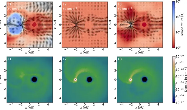
Table 2: Simulation parameters. The values ofMa,Mdand ˙Mdare the same for all simulations.
# a v∞ v∞/vorb Ra Cooling mg h¯ n
Test models
T1 3 15 0.41 20.8 Adiabatic 10−10 0.24 (0.16–0.40) 2×10⁵
T2 3 15 0.41 20.8 Isothermal 10−10 0.12 (0.01–0.36) 2×10⁵
T3 3 15 0.41 20.8 Bowen+Schure 10−10 0.13 (0.01–0.37) 2×10⁵
Test resolution
R1 5 15 0.53 34.7 Bowen+Schure 10−11 0.13 (0.01–0.25) 3.3×10⁶
R2 5 15 0.53 34.7 Bowen+Schure 4×10⁻¹¹ 0.20 (0.02–0.39) 1.1×10⁶ R3 5 15 0.53 34.7 Bowen+Schure 8×10⁻¹¹ 0.26 (0.03–0.49) 5.6×10⁵
Science models
V10a5 5 10 0.35 34.7 Bowen+Schure 2×10⁻¹¹ 0.17 (0.06–0.29) 2.2×10⁶
V15a5 5 15 0.53 34.7 Bowen+Schure 2×10⁻¹¹ 0.16 (0.01–0.32) 2.2×10⁶ V30a5 5 30 1.06 34.7 Bowen+Schure 2×10⁻¹¹ 0.29 (0.14–0.45) 2.2×10⁶
V150a5 5 150 5.31 34.7 Bowen+Schure 2×10⁻¹¹ 0.50 (0.27–0.78) 2.2×10⁶ V19a3 3 19.33 0.53 20.8 Bowen+Schure 2×10⁻¹¹ 0.07 (0.004–0.22) 106
Test sink radius V10a5s2 5 10 0.35 20.8 Bowen+Schure 8×10
−11 0.14 (0.01–0.43) 5.6×10⁵
V15a5s2 5 15 0.53 20.8 Bowen+Schure 2×10⁻¹¹ 0.08 (0.004–0.28) 2.2×10⁶ V30a5s2 5 30 1.06 20.8 Bowen+Schure 2×10⁻¹¹ 0.28 (0.14–0.45) 2.2×10⁶
Notes.The second column corresponds to the name of the model.ais the initial orbital separation of the system in AU.v∞is the assumed terminal
velocity of the wind in km s−1. The ratiov
∞/vorbis the ratio of the terminal velocity to the orbital velocity of the system.Rais the radius of the sink in R. Column 7 specifies the EoS for the model.mgcorresponds to the mass of the SPH particles in units of M. ¯hcorresponds to the mean smoothing length of the SPH particles within radiusafrom the center of mass of the system in units of AU. The numbers brackets correspond to the 95% confidence interval, i.e. 2.5% of the particles have values below the lower limit and 2.5% particles have values above the upper limit of the given interval. The final column gives the total number of particlesngenerated at the end of the simulation.
a few simulations with a smaller sink radius (see Table2). Each simulation was run for eight orbital periods.
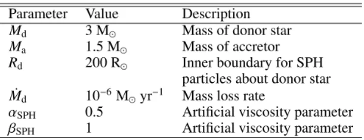
3.4. Testing the method
In this subsection, we compare our simulations (models T1, T2, T3 in Table2) with those ofTheuns & Jorissen(1993). The top panel of Figure1shows the velocity field of the gas in they=0 plane, perpendicular to the orbital plane, for models T1, T2 and T3 after 7.5 orbits. The colormap shows the temperature of the gas in they =0 plane. The donor star is located at x =1 AU,
z=0 AU and the companion star atx=−2 AU,z=0 AU. Gas expands radially away from the primary star. Similar toTheuns & Jorissen(1993), in the adiabatic case (model T1) we observe a bow shock close to the companion star where high temperatures are reached. The high-temperature regions are located symmet-rically above and below the star in this plane. The gravitational compression of the gas by the companion also enhances the tem-perature in this region, expanding the gas in the vertical direc-tion and preventing it from creating an accredirec-tion disk. On the other hand, when an isothermal equation of state is used (model T2), an accretion disk is formed around the companion. In addi-tion, two spiral arms are observed around both systems similar to those observed byTheuns & Jorissen(1993). These features can be seen in the bottom panel of Figure1, where density in the or-bital plane (z=0) is shown. Model T3 shows that using an EoS that includes cooling of the gas (Equation7) gives a similar out-flow structure as in the isothermal case, including the formation of an accretion disk. However, in this model there is an increase in temperature where the spiral shocks are formed. These effects are also found in our science simulations, which we describe in detail in section4.2.
3.5. Mass accretion rate and angular momentum loss
We measure the mass accretion rate by adding the massesmgof
the gas particles that entered the sink during each timestepδtin
the simulation. Due to the discreteness of the SPH particles, the resulting accretion rates will be subject to shot noise. This can be seen as fluctuations in the mass accreted as a function of time. In order to suppress statistical errors in the results, we average the mass accretion rate over longer intervals of time.
Measuring the angular momentum loss rate from the system is more complicated. An advantage of SPH codes is that they conserve angular momentum extremely well compared to Eule-rian schemes (Price 2012). One question that arises is at which distance an SPH particle is no longer influenced by the gravita-tional potential of the binary system. In order to determine this, we construct spherical shells at various radii rS from the
cen-ter of mass of the binary. In the same way as for the accretion rate, we compute the net mass-loss rate through such a surface. Each particleicarries angular momentumJi, of which we add
up the componentsJz,ialong thez-axis, perpendicular to the
or-bital plane. We compute the specific angular momentum of the outflowing mass as follows,
jloss =
PN
i Jz,i
∆Nmg
, (10)
with∆Nthe number of particles that crossed the shell during a timestep∆t. Similar to the accretion rate, we average the mass and angular-momentum loss over longer intervals of time to sup-press statistical fluctuations. We also verified that, once the sim-ulation has reached a quasi-steady state, the orthogonal (xandy) components of the angular momentum-loss are negligible.
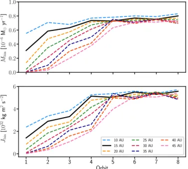
In Figure2 we show the resulting average mass and angu-lar momentum-loss per orbit in our standard model V15a5 (see Table 2) as a function of time for different shell radii rS.
Af-ter several orbits, both quantities become approximately con-stant in time and almost independent of the chosen shell radius. This steady state is reached later for larger radii, correspond-ing to the longer travel time of the wind particles to reach this distance from the donor star. The near-constancy of the angular-momentum loss rate as a function ofrSindicates that the torque
50 km s
14
2
0
2
4
x [AU]
4
2
0
2
4
z [AU]
T1
50 km s
14
2
0
2
4
x [AU]
4
2
0
2
4
z [AU]
T2
50 km s
14
2
0
2
4
x [AU]
4
2
0
2
4
z [AU]
T3
10
310
410
510
6Temperature [K]
4
2
0
2
4
x [AU]
4
2
0
2
4
y [AU]
T1
4
2
0
2
4
x [AU]
4
2
0
2
4
T2
4
2
0
2
4
x [AU]
4
2
0
2
4
T3
10
1710
1610
1510
1410
1310
1210
1110
10De
ns
ity
[g
cm
3
]
Fig. 1:Top:Flow structure in they=0 plane for different EoS after 7.5 orbits. The colormap shows the temperature aty=0. The white arrow on top of the velocity field plots corresponds to the magnitude of a 50 km s−1velocity vector. In the three images we
can observe the wind leaving the donor star radially at x =1 AU. The accretor star is located atx =−2 AU. For model T1, the temperatures reached in the region near the companion star are very high preventing material to settle into an accretion disk.Bottom:
The gas density in the orbital plane (z=0) is shown. The accretor is located atx=−2,y=0, and the AGB star at x=1,y=0. In the middle panel we see that for the isothermal EoS (T2) gas in the vicinity of the accretor settles into an accretion disk. When cooling is included (T3), an accretion disk around the companion is also formed.
gas operates inside a few times the orbital separationa. Beyond
rS≈10 AU (≈2a) the transfer of angular momentum to the gas
is essentially complete, and angular momentum is simply ad-vected outwards with the flow. We therefore adopt the the mass and angular momentum loss values measured atrS=3a, which
reach a steady state after about 4 orbits in model V15a5. The time taken to reach the quasi- steady state depends on the termi-nal velocity of the wind, being shorter for larger velocity.
Once a simulation has reached a quasi-steady state, we com-pute the mass accretion efficiencyβ=M˙a/M˙dfrom the average
mass accretion rate over the remaining N orbits in the simula-tion. Similarly, we average the angular momentum loss (Eq.10) over the lastNorbits to compute the value ofη, i.e. the specific angular momentum of the lost mass in units ofa2Ω.
4. Results
We performed 13 different simulations, listed in Table 2, for which we discuss the results in the following subsections. The first three simulations (T1-T3) are performed to test the EoS (see Sect.3.4). The following three simulations (R1-R3) correspond to the test of different SPH resolutions, compared to simulation V15a5 which we consider the standard model. For this model we chose an orbital separation of 5 AU and a terminal velocity of the wind of 15 km s−1. V10a5, V30a5 and V150a5 correspond to simulations with the same orbital separation but different
ve-locities of the wind, either larger or smaller than for the standard case. V10a5s2, V15a5s2 and V30a5s2 correspond to test simula-tions in which we study the effect of assuming a smaller sink ra-dius (Ra=0.06RL,a) on the mass-accretion rate and radius of the
accretion disk. Note that simulation V10a5s2 was performed at a lower resolution than the others. Finally in V19a3 we change the orbital separation to 3 AU, keeping the same ratio of the velocity of the wind to the orbital velocity of the system as in V15a5.
4.1. Convergence test
Choosing the best resolution for SPH simulations is not sim-ple and depends on the physical process under investigation. To determine the optimal resolution within a reasonable com-putational time, we performed four simulations of our standard model in which we vary the mass of the SPH particlesmg(R1,
R2, R3 and V15a5 in Table2). Note that a differentmgalso
im-plies a change in the average smoothing length ¯h of the SPH particles. Table2shows the value of ¯h within a radiusaof the center of mass of the binary, and the 95% confidence interval of smoothing-length values within this radius. The total num-ber of particlesn generated during one simulation is given by
n =M˙dtend/mg. Thus, the number of particles generated for the
lowest resolution (largestmg) isn=5.6×10⁵andn=3.3×10⁶
for the highest resolution (smallestmg). This last simulation ran
0.0 0.2 0.4 0.6 0.8 1.0
1 2 3 4 5 6 7 8
Orbit 0
2 4 6
10 AU 15 AU 20 AU
25 AU 30 AU 35 AU
40 AU 45 AU
˙Mbin
[
10
−
6M
yr
−
1]
˙Jbin
[
10
32
kg
m
2s
−
2]
Fig. 2: In the top panel we show the average mass loss per orbit for the standard model V15a5 measured at different radii from the center of mass of the binary as indicated by different colours. In the bottom panel the corresponding angular-momentum loss rate is shown. The black thick curve forrS=15 AU corresponds
to the radius at which we measure ˙Jbin.
Since the interest of this study is to obtain numerical es-timates for the average mass-accretion efficiency and average angular-momentum loss during the simulation, these were the quantities we used to check for convergence. Figure 3 shows the values obtained for these quantities (as explained in Sec-tion 3.5) as a function of the mass of the SPH particles mg.
The error bars in this figure correspond to five times the stan-dard error of the mean σm, which was estimated by means of σ2
m = 1/NPNi=1σ 2
m,orbi, where σm,orbi is the standard error of the mean per orbit3 andN the number of orbits during which the quasi-steady state has been reached. Since the number of timesteps over which the average is taken is large, the standard error turns out to be very small. This is the reason why we chose to plot five times the value ofσmin Figure3. Because the
sim-ulation with the highest resolution (smallestmg) only ran for 6
orbital periods, and the system reaches the quasi-steady state af-ter 4 orbits, the error in the mean is larger than for the other simulations.
One thing that can be seen from Figure3is that, even though by only a small amount, the accretion efficiency increases with increasing resolution, contrary to whatTheuns et al.(1996) ob-served. However, we note that in their work the accretion rate was computed by setting an accretion radius proportional to the resolution of the SPH particles (in terms of the smoothing length
h), whereas in our case the radius of the sink has the same
con-3 The standard error of the mean per orbit is:
σm,orb= 1
Np
v u tNp
X
i=1
( ˙mi− hm˙i)2,
whereNpis the number of timesteps (t1,t2, ...,tp) into which the orbit is divided, ˙mithe mass accretion rate at timetiandhmi˙ the average mass accretion rate per orbit.
stant value for all our models. On the other hand, the angular momentum per unit mass lost by the system is approximately independent of the resolution.
We also find that the time variability in the mass-accretion rate (described in Sect. 4.2.3) increases with increasing reso-lution. It is not clear why this takes place, but we should bear in mind that this variability could also be an artefact of the nu-merical method. As will be discussed in Sect. 4.2.3 there ap-pears to be a correlation between the accretion disk mass and the mass-accretion rate. Given that the results of SPH simula-tions for accretion disks depend on the formulation of artificial viscosity, we performed a test simulation with the lowest res-olution (mg = 8×10⁻¹¹) adopting artificial viscosity
parame-ters in Fiequal to those used by Wijnen et al.(2016) for their
protoplanetary disk models (αSPH = 0.1 and βSPH = 1). We
find almost the same value for the average mass-accretion rate (β=0.223±0.002, versusβ=0.221±0.002 for simulation R3). With this alternative prescription of artificial viscosity we find similar variability in the mass-accretion rate.
In order to guarantee reliable results within a reasonable computational time, the chosen resolution for the other simula-tions is the one in which the mass of the individual SPH particles ismg=2×10⁻¹¹M. For this simulation, the value ofβdiffers
by 9% compared to the value obtained for the simulation with largest resolution (R1). This is indicative of the numerical accu-racy of the accretion rates obtained in our simulation. By con-trast, the angular-momentum loss rates (η values) we measure differ by<0.4% between simulations at different resolution.
0.20
0.25
0.30
10
11
10
10
m
g
[M ]
0.50
0.52
0.54
Fig. 3: The mean values of theβ andη, relating to mass and angular momentum loss, as a function of the mass of the SPH particles used to test different resolutions for the simulations. The error bars correspond to the overall standard error of the meanσmmultiplied by a factor of 5 for better appreciation.
4.2. Summary of model results
4.2.1. Morphology of the outflow
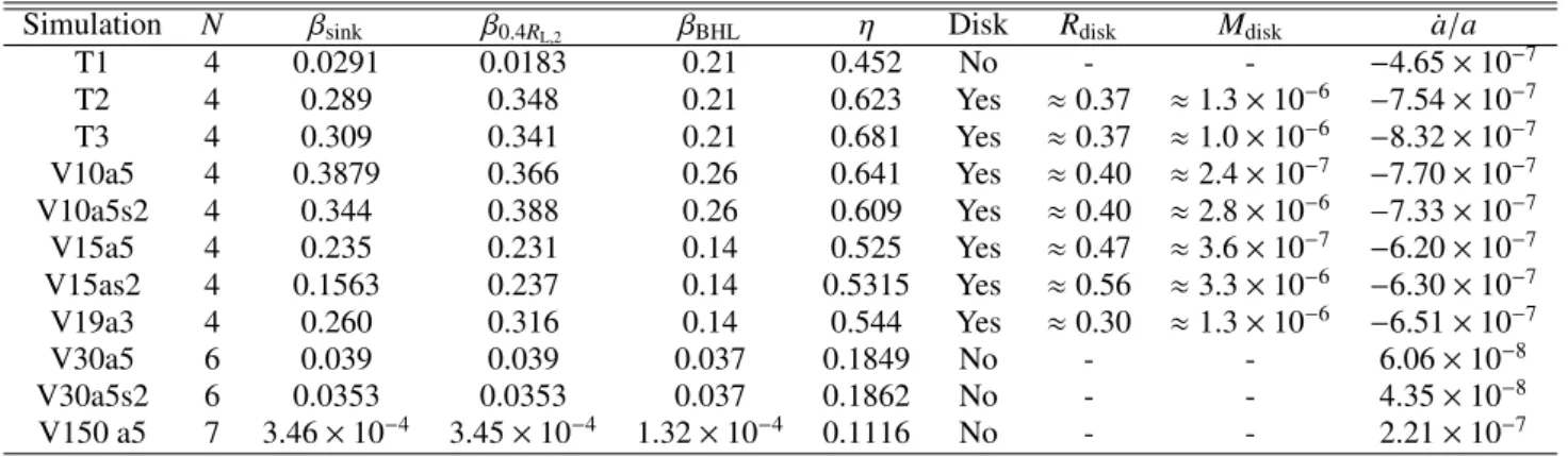
Table 3: Simulation results and orbital evolution parameters
Simulation N βsink β0.4RL,2 βBHL η Disk Rdisk Mdisk a˙/a
T1 4 0.0291 0.0183 0.21 0.452 No - - −4.65×10⁻⁷
T2 4 0.289 0.348 0.21 0.623 Yes ≈0.37 ≈1.3×10⁻⁶ −7.54×10⁻⁷
T3 4 0.309 0.341 0.21 0.681 Yes ≈0.37 ≈1.0×10⁻⁶ −8.32×10⁻⁷
V10a5 4 0.3879 0.366 0.26 0.641 Yes ≈0.40 ≈2.4×10⁻⁷ −7.70×10⁻⁷
V10a5s2 4 0.344 0.388 0.26 0.609 Yes ≈0.40 ≈2.8×10⁻⁶ −7.33×10⁻⁷
V15a5 4 0.235 0.231 0.14 0.525 Yes ≈0.47 ≈3.6×10⁻⁷ −6.20×10⁻⁷
V15as2 4 0.1563 0.237 0.14 0.5315 Yes ≈0.56 ≈3.3×10⁻⁶ −6.30×10⁻⁷
V19a3 4 0.260 0.316 0.14 0.544 Yes ≈0.30 ≈1.3×10⁻⁶ −6.51×10⁻⁷
V30a5 6 0.039 0.039 0.037 0.1849 No - - 6.06×10⁻⁸
V30a5s2 6 0.0353 0.0353 0.037 0.1862 No - - 4.35×10⁻⁸
V150 a5 7 3.46×10⁻⁴ 3.45×10⁻⁴ 1.32×10⁻⁴ 0.1116 No - - 2.21×10⁻⁷
Notes. Nis the number of orbits over which the values are averaged after the quasi-steady state is reached.βsinkis the averaged mas-accretion
efficiency measured from the net sink inflow.β0.4RL,2is the averaged mass-accretion efficiency measured from the net inflow into a shell of radius
0.4RL,2, i.e. it includes the mass inflow of the sink and of the accretion disk, if present.βBHLcorresponds to the mass accretion efficiency as predicted by BHL (Eq.5) withαBHL=1.ηis the averaged specific angular momentum of material lost.Rdiskis the approximate radius of the disk in AU after eight orbital periods, except for model V10a5, where the radius corresponds to 2 orbital periods.Mdiskis the mass withinRdisk. ˙a/ais the relative rate of change of the orbit as derived from Equation3in units of yr−1. Positive sign means the orbit is expanding, whereas negative sign means that the orbit is shrinking.
(V10a5, V15a5, and V19a3), two spiral arms are formed around the system. These spiral arms delimit the accretion wake of the companion star. Similar toTheuns & Jorissen (1993), we find that the inner spiral shock, wrapped around the donor star, is formed by stellar-wind material leaving the AGB star colliding with gas moving away from the companion star with vx > 0.
Near the companion star a bow shock is created by the wind coming from the AGB star as it approaches the accretor. The temperature of the gas in this region increases and material is deflected behind the star forming the outer spiral arm. The Mach number of the flow near the accretor has values between 2 and 6. Because of its proximity to the donor star, where the gas density is high, the inner spiral arm has higher densities than the outer spiral arm. In these systems we also observe an accretion disk around the companion (Sect.4.2.2). The disk is asymmetric and is rotating counterclockwise.
Figure4shows that for model V30a5 the density of the gas in the accretion wake is lower than in models withv∞ <vorb(note
that a different colour scale is used in this panel). The density of the accetion wake is high close to the companion star, but it decreases along the stream. Two spiral arms delineate the edge of the accretion wake, which converge into what appears to be a single arm close to the companion star. No accretion disk is observed in this model. For model V150a5 a single spiral arm is distinguished. The density along this stream is very low, be-cause for simulation V150a5 the gas density is much lower than for the other simulations and only a small fraction of the stellar wind is focused into the accretion wake. Also notice that given the low density of the gas, the effective resolution of this model is lower. Given the large velocity of the wind compared to the orbital velocity of the system, the wind escapes the system with-out being affected by the presence of the companion star and remains spherically symmetric.
If we compare simulations V15a5 and V30a5 we see that the angle formed by the inner high-density spiral arm and the axis of the binary changes as a function of the velocity of the wind. For the low-velocity model, this angle is very sharp and as the wind velocity increases the angle of the stream becomes more oblique. This is expected given that the angle of the accretion wake θ
depends on the apparent wind direction seen by the accretor in its orbit, such that tanθ=vorb/vwind.
4.2.2. Accretion disk
An accretion disk is formed around the accretor in the simula-tions with v∞/vorb < 1 (V10a5, V10a5s2 V15a5, V15as2 and
V19a3). Figure5shows the density of the gas in the orbital plane for the accretion disks formed around the secondaries for simula-tions V10a5, V15a5 and V19a3. One common feature is that the accretion disks are not symmetric. This asymmetry is associated with wind coming from the donor star colliding with material already present in the disk. Another feature in the flow pattern of the simulations is formed by two streams of gas feeding the disk: as seen from the velocity field in the corotating frame (not shown), one stream arises from material moving along the in-ner spiral arm withvx,vy < 0 and the second one comes from
material moving along the outer spiral arm withvx,vy>0.
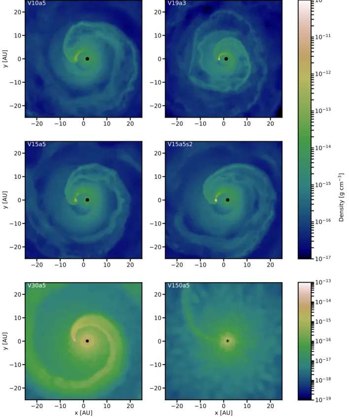
Even though the accretion disk is not symmetric, we approx-imate it as such in order to estapprox-imate its size and mass. We con-struct spheres of different radii centered at the position of the companion star and measure the mass within each sphere as a function of time. The size of the disk is taken as the radius of that sphere outside which the mass is approximately constant as a function of radius. The disk mass is taken as the total gas mass within that sphere. This approach is reasonable because the gas mass inside the spheres is dominated by the mass of the disk. Ta-ble3shows the resulting values of the accretion disk radius and mass for the simulations in which a disk was present after eight orbital periods, except for model V10a5 where the given radius and mass correspond to a time of 2 orbits.
20
10
0
10
20
20
10
0
10
20
y [AU]
V10a5
20
10
0
10
20
20
10
0
10
20
V19a3
20
10
0
10
20
20
10
0
10
20
y [AU]
V15a5
20
10
0
10
20
20
10
0
10
20
V15a5s2
20
10
0
10
20
x [AU]
20
10
0
10
20
y [AU]
V30a5
20
10
0
10
20
x [AU]
20
10
0
10
20
V150a5
10
1710
1610
1510
1410
1310
1210
1110
1010
1910
1810
1710
1610
1510
1410
13De
ns
ity
[g
cm
3
]
Fig. 4: Gas density in the orbital plane (z=0) for V10a5, V10a5s2, V15a5, V19a3, V30a5 and V150a5 after 7.5 orbits.
simulation the disk reaches a larger radius and gradually grows in mass, up to a value at the end of the simulation about 9 times larger than in V15a5 (see Table3). This can be understood as the smaller sink allows gas in the disk to spiral in to closer or-bits around the secondary by viscous effects, transferring angular momentum to the outer regions of the disk which thus grows in size. Such behaviour is physically expected, but simulations with even smaller sink radii and extending over a longer time are
re-quired to investigate the mass and radius of the disk and their possible variability.
1
0
1
x [AU]
1.5
1.0
0.5
0.0
0.5
1.0
1.5
y [AU
V10a5
0
10
20
30
40
Time [yr]
0.0
0.5
1.0
1.5
2.0
2.5
3.0
3.5
Ma
ss
[1
0
7
M
]
V10a5
1
0
1
x [AU]
1.5
1.0
0.5
0.0
0.5
1.0
1.5
y [AU]
V15a5
0
10
20
30
40
Time [yr]
0
1
2
3
4
Ma
ss
[1
0
7
M
]
V15a5
0.5
0.0
0.5
x [AU]
0.75
0.50
0.25
0.00
0.25
0.50
0.75
y [AU]
V19a3
0.0 2.5 5.0 7.5 10.0 12.5 15.0 17.5 20.0
Time [yr]
0.0
0.2
0.4
0.6
0.8
1.0
1.2
Ma
ss
[1
0
6
M
]
V19a3
10
1610
1510
1410
1310
1210
1110
1010
1710
1610
1510
1410
1310
1210
1110
1610
1510
1410
1310
1210
1110
10Fig. 5: The left-hand plots show the density in units of g cm−3 in the orbital plane of the region centered on the accreting star for three models withv∞/vorb <1, zooming in on the accretion disks. The size of the box corresponds to the Roche-lobe diameter of
the companion star. For models V15a5 and V19a3, the situation after 7.5 orbits is shown, whereas for model V10a5 we show the accretion disk before it disappears, but in the same orbital phase. In the right-hand panels we show the disk mass, i.e. the mass contained in a sphere of radiusRdisk(see Table3) as a function of time.
the sink particle. When performing a similar simulation but with a smaller sink radius, V10a5s2, the accretion disk remains for the rest of the simulation and gradually increases in mass, sim-ilar to what was seen in simulation V15a5a2 discussed above. The size of the disk remains smaller than in the models with a wind velocity of 15 km s−1. A similar pattern is found in model
V19a3 (bottom panel of Figure5), in which the disk mass in-creases with time. A longer simulation will be needed to see if it converges towards a constant value.
For the models in which v∞/vorb > 1, no accretion disk is
by the sink particle without forming an accretion disk. We con-clude that if an accretion disk were to form in this system it will be smaller than the assumed sink radius.
4.2.3. Mass-accretion rate
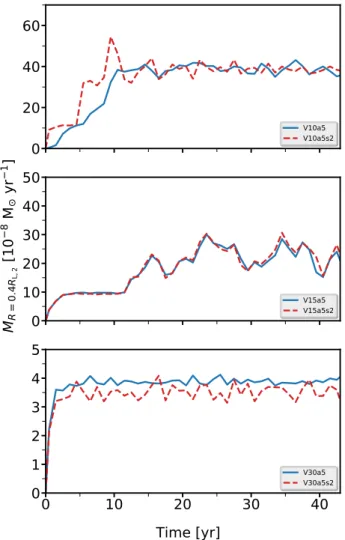
Figure 6 shows the average mass-accretion rate over intervals of one year for models V10a5, V15a5, V30a5 (solid lines), V10a5s2, V15a5s2 and V30a5s2 (dashed lines).
In models V15a5 (middle panel) and V19a3 (not shown), we find a lot of variation in the accretion rate, which clearly exceeds the noise associated with the finite number of particles accreted. This suggests a correlation between the mass of the accretion disk and the accretion rate. This can be observed if we compare the middle right panel of Figure5and the middle panel of Figure
6, where the peaks and troughs in the mass of the disk coincide in time with those observed in the mass-accretion rate. In the case of model V15a5s2, where the mass in the disk gradually increases with time, the accretion rate as a function of time also shows an increase (dashed line in the middle panel of Fig.6). The average accretion rate for model V15a5s2 is a factor of 1.5 lower than for model V15a5 where the sink radius is larger. For model V10a5 (top panel of Figure6), we find that after the accretion disk becomes smaller than the sink and is swallowed, the vari-ation in the accretion rate decreases. For model V10a5s2 with a smaller sink, although the accretion disk is present for the en-tire simulation, the variability in the accretion rate is smaller than for model V15a5s2 (where the accretion disk is also present over the entire simulation). However, we should note that the resolu-tion for model V10a5s2 is much lower. Similar to models V15a5 and V15a5s2, the mass-accretion efficiency is lower for model V10a5s2 than for model V10a5. In the bottom panel of the same figure, we show the accretion rate for model V30a5. Apart from the Poisson noise associated with the finite resolution of the SPH simulations, the accretion rate is constant in time. For the same simulation but with a smaller sink we find a slightly lower accre-tion efficiency.
We find that the mass that is not accreted in models V10a5s2 and V15a5s2 is stored in the accretion disk. Figure7shows the net mass inflow rate into a shell of radius 0.4RL,2around the
sec-ondary for models V10a5, V15a5 and V30a5 (solid lines) and their corresponding models with a smaller sink radius (dashed lines). The chosen shell radius is larger than the size of the ac-cretion disk in all the simulations, so that the inflow rate corre-sponds to the total mass-accumulation rate of the sink and the disk, ˙M0.4RL=M˙sink+M˙disk, since the amount of gas within this
volume that isnotin the disk is very small. In the steady state, the inflow rate we find in this way is insensitive to the chosen sink radius. For simulations V15a5 and V15a5s2, this combined ac-cretion rate is seen to be very similar and also shows similar vari-ability over time. A similar feature holds for simulation V10a5 and V10a5s2. Since it is likely that the mass in the disk will even-tually reach the stellar surface, this may be a better measure of the steady-state accretion rate that is insensitive to the assumed sink radius. In the case of models V30a5, V30a5s2, we observe the same small discrepancy in the inflow rate atR=0.4RL,2that
we find in Figure6. The net influx of mass within the shell is the same in both simulations, reflecting the steady-state condi-tion reached. However, when the sink radius is larger it captures material that may otherwise escape. Therefore, for simulations such as V30a5 in which no accretion disk is formed, our results provide only an upper limit to the amount of mass accreted.
In order to determine the long term evolution of the orbit, one of the quantities of interest from these simulations is the
average mass-transfer efficiencyβ. Given the results discussed above and shown in Figures6and7, we take the mass-transfer efficiency as β0.4RL = M˙0.4RL/M˙d. In Table 3, we provide the
mean values of this quantity for the science simulations, as well as the mean values for the material captured by the sink only, i.e.βsink = M˙sink/M˙d. In Figure8, we show the corresponding
values for the accretion efficiencyβ0.4RLas a function of the ratio
v∞/vorbfor the science simulations. The dotted line corresponds
toβBHL in equation 5 withαBHL = 1. Solid dots in the figure
correspond to models V15a5-V150a5 and stars to models T3 and V19a3, both of which havea=3 AU.
Model V150a5, in which we use a wind velocity ten times larger than the typical velocities of AGB winds, was set up to approximate the isotropic wind mode. Figure 8shows that for this model, our numerical result for the accretion efficiency ex-ceeds the expected value for BHL accretion by a factor of 2.5 (see also Table3). However, we note that the BHL accretion ra-dius for this simulation is smaller than the rara-dius of the sink, which will result in a discrepancy with the BHL prediction for the accretion efficiency. The dashed line in the same figure corre-sponds to the accretion efficiencyβsinkassuming the geometrical
cross section of the sink instead of the BHL cross section. The difference between the simulation result andβsinkis reduced to a
factor of 1.3.
Fig.8shows several interesting features. As the ratiov∞/vorb
increases, the value ofβdecreases, following a similar trend as expected from BHL accretion. However, forv∞/vorb<1 we find βvalues that exceed theβBHLby up to a factor of 1.5-2.3. For
the lowest wind velocity, the mass transfer efficiency is approxi-mately 40%. Finally, for models V15a5 and V19a3, which have the samev∞/vorbratio, the accretion efficiencies shown in Figure
7differ by a factor of 1.4.
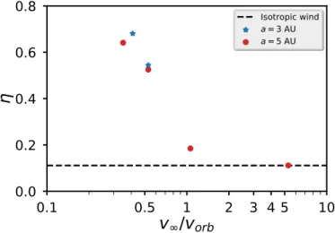
4.2.4. Angular-momentum loss
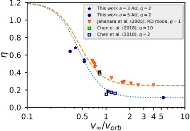
The second quantity of interest resulting from our simulations is the value of the specific angular momentum of the material lost by the system. Figure9shows the values of this quantity in units ofJ/µas a function ofv∞/vorbfor the different models. We
see that the smaller the velocity of the wind, the larger the spe-cific angular momentum of the material lost. This is consistent with the expectation that when the velocity of the wind is small compared to the relative orbital velocity of the system, more in-teraction between the gas and the stars occurs and more angular momentum can be transferred to the gas. This strong interaction is also seen in the large mass-accretion efficiency, as well as in the existence of a large accretion disk and in the structure of the spiral arms of the systems. The simulations withv∞<vorbshow
spiral arms that are more tightly wound around the system, and with higher gas densities, than the simulations for higher wind velocities (see Sect.4.2.1and Fig.4). These spiral arms corre-spond to the accretion wake of gas interacting with the secondary star. We interpret the loss of angular momentum as the result of a torque between the gas in this accretion wake and the binary system. The magnitude of this torque depends on the orientation of the wake and the density of the gas behind the companion star. When the accretion wake is approximately aligned with the binary axis and the density in the wake is relatively low, as in simulations withv∞/vorb > 1, the torque between the gas and
the binary will be small. The torque exerted on the gas will in-crease as the wake misaligns with the binary axis, and as the gas density in the accretion wake becomes higher. Both these effects occur for low values ofv∞/vorb, in particular in the inner spiral
0
20
40
60
V10a5 V10a5s2
0
10
20
30
40
50
V15a5 V15a5s2
0
10
20
30
40
0
1
2
3
4
5
V30a5 V30a5s2
Time [yr]
Ma
ss
ac
cr
et
ion
ra
te
[1
0
8
M
yr
1
]
Fig. 6: The average accretion rate over one-year intervals for models V15a5 (top), V10a5 (middle) and V30a5 (bot-tom) is shown in blue. The dashed red lines correspond to the year-averaged mass accretion rate for the corresponding models with a smaller sink radius.
0
20
40
60
V10a5 V10a5s2
0
10
20
30
40
50
V15a5 V15a5s2
0
10
20
30
40
0
1
2
3
4
5
V30a5 V30a5s2
Time [yr]
M
R=
0.
4R
L,2
[1
0
8
M
yr
1
]
Fig. 7: The net inflow rate into a sphere of radius 0.4RL,2
around the accretor star averaged over intervals of one year for the same models as in Figure6.
to the binary axis (Fig.4).Therefore, the transfer of angular mo-mentum from the orbit to the outflowing gas increases strongly with decreasingv∞/vorb.Furthermore, it implies that most of the
angular-momentum transfer occurs at short distances from the binary system, as is confirmed by the test discussed in Section
3.5(see Figure2).
Model V150a5 approximates the isotropic or fast wind mode fairly well. In this case, the ejected matter escapes from the sys-tem with very little interaction, only removing the specific angu-lar momentum of the orbit of the donor star. For this simulation, the value we obtained forηisηnum=0.112±0.001, very close to
the expected value for the mass ratio of the stars in our models,
ηiso=0.111 (dotted line in Fig.9).
An interesting result of our models is that for the same value ofv∞/vorb, but different orbital separations, the specific angular
momentum of the mass lost is very similar. For models V15a5
η≈0.52 and for V19a3,η≈0.54. Model V10a5 has the largest loss of angular momentum among the high-resolution simula-tions withη =0.64, although the low-resolution simulation T3 has an even large amount of angular-momentum loss,η=0.68.
5. Discussion
5.1. Assumptions and simplifications
A complete study of binary systems interacting via AGB winds requires the simultaneous modelling of hydrodynamics, radia-tive transfer, dust formation and gravitational dynamics. In this study, several simplifications have been made.
5.1.1. Wind acceleration
10
1
10
0
v /v
orb
10
4
10
3
10
2
10
1
10
0
Bondi-Hoyle Rsink
a = 3 AU a = 5 AU
Fig. 8: The fraction of mass accreted by the companion as a func-tion of v∞/vorb. The dotted line corresponds to BHL accretion
rate with αBHL = 1, and the dashed line to the accretion rate
for a geometrical cross section of sizeRsink. Dots correspond to
models in which the orbital separation is 5 AU and stars to mod-els in which a = 3 AU. The values shown are measured at a radius of 0.4RL,2(β0.4RL,2).
0.1
0.5
1
2 3 4 5
10
v /v
orb
0.0
0.2
0.4
0.6
0.8
Isotropic winda = 3 AU a = 5 AU
Fig. 9: The specific angular momentum of the mass lost from the system as a function ofv∞/vorb. The smaller the velocity of
the wind compared to the orbital velocity, the higher the specific angular momentum loss. For equal velocity ratios, the specific angular momentum is very similar. The dashed line shows the valueηisoexpected for an isotropic wind for a mass ratioq=2.
2018). For the orbital parameters assumed in our models,Rdustis
similar to or larger than the Roche-lobe radius of the donor star,
RL,1. As described inMohamed(2010) andAbate et al.(2013),
in this situation mass transfer can occur by WRLOF, i.e. by a dense flow through the inner Lagrangian point into the Roche lobe of the companion. However, given that the wind particles in our simulations are injected with predefined terminal velocities from the radius of the donor star, no WRLOF is observed.
If the gradual acceleration of the wind is taken into account, the density and velocity structure of the gas inside the orbit of the companion will be different which may affect the outflow morphology in our low wind-velocity simulations. To some ex-tent the effects of wind acceleration can be accounted for by as-suming an increasing velocity profile in Eq. 6, mimicking the
velocity profile of an AGB wind. The resulting acceleration in such models would still be spherically symmetric. In addition, the modified outflow in a binary can change the optical depth of the dust and thus affect the acceleration of the wind itself, making it non-isotropic. This can only be studied by explicitly modelling dust formation and radiative transfer in wind mass-transfer simulations (e.g. seeMohamed & Podsiadlowski 2012;
Chen et al. 2017) and is beyond the scope of the present study. For this reason, and although the simulations presented here give insight into the dependence of the angular-momentum loss and the accretion efficiency on thev∞/vorb ratio, our results should
be interpreted with some caution.
5.1.2. Accretion
Given the small radius of a main-sequence or white-dwarf com-panion star, resolving it spatially would be very computationally demanding. For this reason the accretor was modelled as a sink particle with radius equal to a fraction of the size of its Roche lobe. In the simulations where an accretion disk is formed, the in-ner disk radius is limited by the sink radius. However, physically there is no reason to expect that the disk will not extend inwards to the stellar radius by viscous spreading, and any gas captured in the disk will be transferred towards the stellar surface. As we have shown in Section4.2.3, the sum of the accretion rate onto the sink and the mass accumulation rate in the disk appears to be independent of the assumed sink radius, and should give a reliable measure of the mass transfer rate to the companion. On the other hand, we cannot be sure that all matter that approaches the surface of the star through the disk will be accreted, as some fraction of it may be expelled by a wind or jet formed in the inner part of the accretion disk. In simulations with larger wind veloc-ities where we do not find an accretion disk, it is possible that a disk is still formed at a smaller radius within the sink. However, some of the mass captured within the sink may not end up in the disk and reach the surface of the companion. For these reasons, and although our results for the mass accretion efficiency with different prescriptions for the artificial viscosity and sizes of the sink particle seem to converge, the values provided should be taken as upper limits.
5.1.3. Angular-momentum transfer