5455.pdf

(1)

New statistical learning methods for chemical

toxicity data analysis

by

Chaeryon Kang

A dissertation submitted to the faculty of the University of North Carolina at Chapel Hill in partial fulfillment of the requirements for the degree of Doctor of Philosophy in the Department of Biostatistics.

Chapel Hill 2011

Approved by:

Michael R. Kosorok Yufeng Liu Fred A. Wright

(2)

c

(3)

Abstract

New statistical learning methods for chemical toxicity data analysis. (Under the direction of Michael R. Kosorok.)

In the first part of the dissertation, we introduce the “change-line” classification and regression method to study latent subgroups. The proposed method finds a line which optimally divides a feature space into two heterogeneous subgroups, each of which yields a response having a different probability distribution or having a different re-gression model. The procedure is useful for classifying biochemicals on the basis of toxicity, where the feature space consists of chemical descriptors and the response is toxicity activity. In this setting, the goal is to identify subgroups of chemicals with different toxicity profiles. The split-line algorithm is utilized to reduce computational complexity. A two step estimation procedure, using either least squares or maximum likelihood for implementation, is described. Two sets of simulation studies and a data analysis applying our method to rat acute toxicity data are presented to demonstrate utility of the proposed method.

Second, the asymptotic properties in the change-line regression model are studied through empirical process techniques, including consistency and the rates of con-vergence of M-estimators in the change-line regression model. We prove that the estimator of the regression parameters achieves √n-consistency while the estimator of the change-line parameters are n-consistent.

(4)

(5)

Acknowledgments

It is a pleasure to thank many people who made this thesis possible.

First and foremost, I would like to express my sincere appreciation and gratitude to my advisor, Dr. Michael Rene Kosorok, for his support, financial assistance, and constant encouragement. Throughout my dissertation research period, he provided invaluable suggestions and good teaching. He made me believe that theory and ap-plication are not separate, rather, theory helps us to solve practical problem better.

I gratefully thank the members of my committee. I thank Dr. Yufeng Liu for his advice and help for computational problems in this research. I gratefully thank Dr. Fred A. Wright for constant encouragement and insightful comments on this thesis. My sincere thanks go to Dr. Hao Zhu for providing me the chemical toxicity data sets and helping me understand them better. Many thanks go in particular to Dr. Fei Zou for her invaluable comments and advice for this thesis.

My special thanks go to Dr. Donglin Zeng. He constantly encouraged me in my first and second years in UNC at Chapel Hill as my academic advisor, and patiently answered my questions about BIOS 760.

I would like to thank Dr. Jianwen Cai (Clinical and Translational Science Award),

(6)

Dr. Robert M. Hammer, Dr. John H. Gilmore (UNC Schizophrenia Research Cen-ter) and NC Center for Childrens Health Improvement for an excellent opportunity to work with them as a graduate research assistant (GRA) student. I also thank Dr. Chirayath M. Suchindran for his support and advice. I would like to acknowledge the advice and help of Dr. Gary Koch, Dr. Amy Herring, Dr. Bahjat Qaqish and Dr. Todd Schwartz for my GRA research. I also would like to thank Kosorok Research Group (KRG) and Statistical Learning and High-Dimensional Data (SLHDD) work-ing group for helpful discussion.

(7)

List of Figures

3.1 Plots for the change-line classification under various sample sizes . . . 41

3.2 RLOWESS curves for simulated data . . . 42

3.3 Plots for the change-line regression under various sample sizes . . . 44

3.4 Density plot under various scenarios . . . 45

3.5 Projection pursuit regression plot . . . 51

3.6 Change-line classification for the chemical toxicity data . . . 57

3.7 RLOWESS curves for the chemical toxicity data . . . 59

4.1 Figures to prove Claim 3 . . . 77

4.2 The first figure to prove Claim 4. . . 83

4.3 The second and third figures to prove Claim 4. . . 85

5.1 Flowchart of the IDC method withM feature categories. . . 99

5.2 Average prediction accuracies . . . 109

5.3 Result of the ToxRefDB data set . . . 117

5.4 Result of the ICCVAM data set . . . 118

6.1 Histogram and density plot of ˆα and ˆγ . . . 142

6.2 Scatter plots of ˆα against ˆγ . . . 142

6.3 2D contour plots (1) of ˆα and ˆγ . . . 143

6.4 2D contour plots (2) of ˆα and ˆγ . . . 143

6.5 3D contour plots of ˆα and ˆγ . . . 143

(12)

List of Tables

2.1 Interaction Tree . . . 13

3.1 Change-line classification under various sample sizes . . . 40

3.2 Change-line regression under various sample sizes . . . 43

3.3 Change-line classification for three different scenarios . . . 47

3.4 Change-line regression without heterogeneous subgroups . . . 48

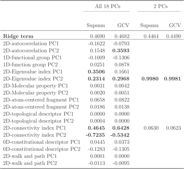
3.5 The estimates from projection pursuit regression . . . 52

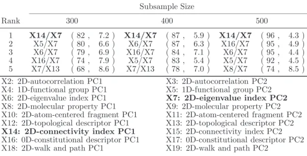
3.6 Top 5 pairs of PCs for the chemical toxicity data . . . 55

3.7 Change-line classification for the chemical toxicity data . . . 56

3.8 Simulation results of the hypothesis test . . . 66

5.1 Averages and standard error estimates . . . 108

5.2 Frequency of the selected base classifiers . . . 111

5.3 All endpoints for the chemical toxicity . . . 113

5.4 Ten categories of chemical descriptors. . . 114

5.5 Summary statistics for ToxRefDB and ICCVAM data . . . 119

5.6 The number of base classifiers to be combined . . . 122

5.7 The variation of the system size within CV . . . 123

5.8 Frequency of the selected base classifiers with SVM . . . 126

5.9 Frequency of the selected base classifiers with random forests . . . 127

5.10 Frequency of the selected base classifiers with Adaboost . . . 128

6.1 Change-line classification using probabilistic working model . . . 135

6.2 Probabilistic working model under various initial values for EM . . . . 137

(13)

6.4 Empirical validation of the rate of convergence . . . 144

(14)

Chapter 1 Introduction

In medicinal chemistry and toxicology, the assessment of potential toxicity associated with drugs and commercial chemicals is an important topic. Some of the chemicals may be hazardous to human health or to the environment. Standard toxicity assess-ment requires in vivo testing in animals, which is expensive, time consuming, and raises ethical concerns. For these reasons, only a small fraction of commercial chem-icals have been tested extensively. Thus, there is increasing interest in developing models for accurate toxicity prediction, to better prioritize chemicals for testing, with an ultimate goal of purely computational toxicity prediction. Quantitative Structure-Activity Relationship (QSAR) modeling is one of the most popular approaches to develop computational toxicity models [Richard, 2006]. QSAR approaches model the relationship between chemical structures and target biological activities and the re-sulting models are used to predict the target biological activities using the chemical descriptors of new compounds.

(15)

the size and complexity of biomedical data. These biomedical data contain rich in-formation about complex human diseases and biological processes that allows us to better understand disease mechanisms and to provide better treatment to patients. The problem is how to extract underlying information contained in such massive amounts of data. Statistical learning is widely used to resolve statistical problems that we face when we use high-dimensional and complex data. According to Hastie et al. [2009], “statistical learning can be broadly described as a statistical approach to extract important patterns and trends and understand ‘what the data says.’ We call this learning from the data.” Statistical learning can provide a useful tool not only to answer specific research questions but also to make discoveries that formulate new hypothesis. Statistical learning problems can be categorized as either super-vised learning (for example, classification or prediction of outcomes) or unsupersuper-vised learning (for example, clustering observations based on characteristic features). In this dissertation, we study two specific problems: heterogeneous latent subgroups in a population and the low-prediction accuracy of classification models. We propose two new statistical learning procedures to study these two problems, and apply those methods to improve QSAR models of animal toxicity.

1.1 The change-line method

It is scientifically reasonable to expect the relationship between toxicity activity and chemical descriptors to depend on some latent structure within the population. For example, there may be two groups of chemicals with normally distributed response (toxicity activity) values, one group with large mean and small variance and another group with small mean and large variance. In investigating such associations, it is also possible that a group of chemicals shows a positive relationship between toxicity

(16)

activity and a set of descriptors while another group of chemicals shows a negative relationship with the same descriptors. In such cases, we cannot identify the impor-tant latent structure using traditional classification and regression methods.

To address this latent classification and regression problem, we consider first the case in which the sample size is n, the feature space is p−dimensional, and there are only two latent groups separated by ap−dimensional hyperplane. Even in this appar-ently simple case, the computational complexity is prohibitive, even with moderate to small sample sizes. For this reason, we focus in this preliminary paper on the very simple setting where the feature space is two-dimensional and the latent subgroups of interest are divided by a line which we call the change-line. This simple initial imple-mentation will pave the way for the more general, higher dimensional methodology. When each group has a different probability distribution in the response, we call the approach “change-line classification” and focus on finding the line that divides the complete population into two subgroups and estimates the distribution parameters of the two groups. When each group has a different association between the response variable and a set of covariates (some of which may be also contained in the feature space), we call the approach “change-line regression” and focus on finding a line about which the regression parameters differ.

(17)

there have been numerous studies on the change-point problem in parametric, non-parametric, seminon-parametric, and Bayesian settings. However, when we consider the change-line setting where X ∈ R2_{, significant computational challenges arise} com-pared to the one-dimensional change-point problem. There have been a few studies considering the change problem in the two-dimensional case, but the approaches were not applicable to the general two-dimensional setting. The method we propose, in contrast, enables a general extension of the one-dimensional change-point problem to the change-line problem in a two-dimensional feature space.

When the response variable is binary, e.g.,Y ∈ {1,−1}, the problem can be roughly viewed as “latent classification” from machine learning. However, one can apply the latent classification method only when the response variable is binary (or at least categorical). Compared to the classical “latent classification” problem, our approach is more applicable to a broader range of response possibilities in the sense that it is applicable to both continuous and discrete response variables. Moreover, the pro-posed method combines some ideas from machine learning with statistical modeling. Thus, we can potentially reduce the non-reproducibility problem of the pure machine learning method using principled statistical inference and modeling methodology.

An alternative approach is to apply project pursuit regression (PPR, Friedman and Stuetzle [1981]) or support vector regression (SVR, Vapnik et al. [1996]) to analyze these types of data. Compared to PPR or SVR, the proposed change-line approach can more easily handle the setting where the feature space variablesX differ from the regression variables Z. This appears to be impossible for SVR. On the other hand, PPR could potentially be generalized to allow changing coefficients in a regression on

Z, where the change is a linear function of the feature space X. We do not pursue

(18)

this avenue further here.

A potential application for the change-line approach is development of person-alized medicine. Recently, there has been great interest in developing personperson-alized medicine in clinical trials. Some recent studies have shown that people can respond to the same treatment in different ways due to individual characteristics. For exam-ple, a recent study by Glynn et al. [2009] for the National Cancer Institute (NCI) found that a genetic variation located in the SOD2 gene is associated with different responses to the chemotherapy drug cyclophosphamide, which is used to treat breast cancer. Our method would be useful in studying heterogeneous subgroups of patients who respond to the treatments differently.

1.2 The interactive decision method

(19)

interactive method). It is scientifically reasonable to assume that different feature categories may be interactively associated, and that such relationships could affect the classification task.

In this dissertation, we propose the interactive decision committee (IDC) method to improve prediction accuracy in binary classification problems when high-dimensional feature variables are grouped into feature categories. The method uses the interac-tive relationships between existing feature categories to build base classifiers in the decision committee context. This is our first contribution. Our second contribution is to utilize a two-stage 5-fold cross-validation (CV) technique to choose the number of base classifiers to be combined. This technique reduces problems on overtraining by controlling the size of the decision committee method. In addition, we applied stacked generalization to learn a combination rule. We found that this procedure can improve classification performance compared to a single large, unaggregated classifier.

1.3 Outline of thesis

The rest of this dissertation is organized as follows. In Chapter 2, we provide a sum-mary of the literature review of the existing approaches to solving similar problems to the one described above. This includes an introduction of an efficient algorithm to consider all possible lines generated by two points in a two dimensional feature space. For the IDC method, a general setting for the decision committee method and aggregation rules, stacked generalizations, and a brief introduction to Support Vec-tor Machines, Random forests, and AdaBoost algorithms are provided. In Chapter 3, we describe a model and method for the change-line classification and regression

(20)

(21)

Chapter 2 Background

2.1 Change-line method

2.1.1 Projection pursuit regression

(22)

aspects, the change-line classification and regression method is similar to PPR. PPR is a type of nonparametric smoothing method, and it approximates the regression surface by a sum of general smooth functions of linear combinations of the predictors in an iterative way.

Let {X, Y}n

i=1 be a pair of random variables such that X is a random vector in

Rp_{, and} _Y _{is a response variable in}_R_{. Let} _ω

m, m=1,2, . . . , M be a unit p-vector of

unknown parameters. Then, the PPR model can be defined as f(X) =

M

∑

m=1

gm(ωmTX),

where gm(ωTX) is a ridge function, ωTms are projection direction vectors, and M

denotes the number of projections. M can be determined in various ways such as cross-validation or a forward stage-wise strategy that stops adding terms when the newly added term does not significantly improve the model. Basically, PPR finds the

gm and ωm that minimize the objective function n

∑

i=1 [ri−

M

∑

m=1

gm(ωmTxi)]2, (2.1)

where ri is a residual, and it is initialized to yi. Let us consider the simplest case of

one-dimensional PPR (M =1). PPR can be accomplished in a two-step procedure. For the first stage, given the direction vector ωand v={vi}={ωTxi}n_i₌₁, we construct

a smooth representation g(v) of the current residual as ordered in ascending values of v. It is usually obtained by a one-dimensional smoothing method such as local regression or the smoothing spline method so as to minimize (2.1). Next,ωis obtained by the use of a quasi-newton method as follows: let ˆω(k) _{be the estimate of}_ω _{at the}

kth _{iteration. By the quasi-newton method, we can write} _g(_ω_ˆ(k+1)T_x

i) ≈ g(ωˆ(k)Txi)

+g′(_ω_ˆ(k)T_x

(23)

as

n

∑

i=1[

ri−g(ωˆ(k+1)Txi)]2 ≈ n

∑

i=1

g′(ωˆ(k)Txi)2[ωˆ(k)Txi+

ri−g(ωˆ(k)Txi)

g′(_ω_ˆ(k)T)_x i −

ˆ

ω(k+1)Txi]2.

Thus, ˆω(k+1) _{can be estimated by weighted least squares regression with new a} re-sponse variable ˆω(k)T_x

i+

ri−g(ωˆ(k)Txi)

g′(_ω_ˆ(k)T_x i)

on thexi with weights g′(ωˆ(k)Txi)2 without

intercept. Once we find the direction vector ˆω(k+1)_{and ˆ}_v(k+1)

i =ωˆ(k+1)Txi, we can

com-pute the correspondingg(vˆ(k+1)T)_{. This process is repeated until the improvement in}

(2.1) is not significant compared to a user-defined threshold.

Huber [1985] and Hastie et al. [2009] discussed some shortcomings of PPR. One of the difficulties of PPR is interpretation of the fitted model. The results of one-dimensional PPR can be understandable as similar to linear regression, but it is not easy to interpret how a single term of projection affects the approximation in higher dimensional PPR (M ≥2). For this reason, PPR is useful for prediction rather than modeling of data except for one-dimensional PPR. Also, since PPR is a linear dimen-sion reducer, it works poorly in the case where a highly nonlinear structure exists in the data [Huber, 1985]. The demanding computational problem could be solved by newly developed efficient algorithms, but PPR is still a computationally expensive method. Although PPR itself is not widely used to solve statistical problems, it af-fects the development of new methodologies such as neural networks from machine learning and independent component analysis (ICA) which is a very popular method of analyzing brain images [Hastie et al., 2009].

(24)

2.1.2 Latent classification/Latent class regression

The change-line classification and regression model could be thought as a “binary

latent variable” model. That is, the distribution of the observations depends on a

binary latent variable, and this variable is completely determined by a line. Extensive literature exists on the latent class model or latent variable model: the following are two articles of particular interest.

Recently, Langseth and Nielsen [2005] developed the “latent classification model (LCM)”, which is a family of classifiers for a categorical response variable and a set of continuous attributes. LCM combines a naive Bayes model with a mixture of factor analysis (FA). FA reduces the dimensionality of the attributes space based on the covariance structure of the data. As a result, LCM produces a relatively small model, and it utilizes a set of latent variables to model correlations between attributes, which is not allowed in the classical naive Bayes method. Let Y be a categorical response variable,X be a set of continuous attributes, andZ be a set of latent variables which is also continuous. Conditionally onY =j, the latent variableZ is assumed to follow a Gaussian distribution and to be conditionally independent. Similarly, conditional on

Z =z, X is assumed to follow a Gaussian distribution independently. Langseth and Nielsen [2005] showed that whenever X∣ Y =j follows a Gaussian distribution, the joint distribution(Y, X)can be represented by an LCM. To learn the LCM classifier, the authors proposed an algorithm to score a model based on its accuracy, which is estimated by using a wrapper approach. Also, an Expectation-Maximization (EM)-algorithm was utilized to learn the model parameter in the Gaussian distribution for

(25)

and principle component analysis (PCA), the proposed LCM showed the best per-formance, and it produced a simpler model. In a later paper, Langseth and Nielsen [2009] extended the LCM to binary LCM by allowing binary attributes with contin-uous latent variables.

Guo et al. [2006] presented a regression model where both the categorical outcome and the continuous predictors are latent. For individual i, one is interested in the relationship between a q−dimensional continuous variable fi and a categorical

vari-able ci with K categories. However, neither fi nor ci is directly observable. Instead,

we observe a p−dimensional continuous vector X and j−dimensional binary response vectorYi to measurefi andci, respectively. In this article, the latent variables(fi, ci)

were assumed to be missing data, and two numerical methods were utilized to ob-tain maximum likelihood estimators: the Monte-Carlo Expectation and Maximization (MCEM) algorithm and the Gaussian quadrature approximation with a quasi-newton algorithm. Similar to the latent classification models, Yi is assumed to be

condition-ally independent of Xi given ci = c and fi = f. This implies that Yi and Xi are

related only through the relationship of ci and fi. Additionally, the latent factor fi

is assumed to follow a normal distribution in order to use the Gaussian quadrature approach.

Both the LCM and latent class regression methods were developed based on the assumption that the latent variable is continuous, and the probability distribution of the latent variable is known. This is different from the change-line approach be-cause we are interested in studying binary latent variables without any distributional assumption of a latent variable.

(26)

Table 2.1: Interaction Tree

x≤c∶tL x>c∶tR

Group 1 µL

1,y¯1L, s21, n1 µR1,y¯1R, s22, , n2 Group 2 µL

2,y¯2L, s23, n3 µR2,y¯2R, s24, n4

2.1.3 Subgroup analysis in machine learning

In subgroup analysis, one is interested in finding subgroups in a population that are sufficiently large and have statistically unusual characteristics related to a property of interest. For example, in comparing treatment effects, researchers are interested in the heterogeneity of the treatment effect across subgroups as well as the overall treatment effect. The traditional approach to subgroup analysis is based on test-ing interaction effects between treatment and a covariate of interest. When there exists a significant interaction effect, one evaluates the treatment effect within each subgroup. This approach is simple, but the potential subgroups tend to be subjective.

To avoid such subjectivity, Su et al. [2009] proposed a new subgroup analysis approach that combines the idea of recursive partitioning and an interaction tree (IT) procedure. Suppose we havenindependently and identically distributed observations {yi, zi, xi}, whereyi is a continuous response variable,zi is a binary response variable

for two treatments, and xi =(xi1, . . . , xip)T is a p−dimensional covariate vector. For

a continuous variable x and a threshold value c, observations satisfying x≤ c go to the left child node tL while others go to the right child node tR. Let {µ₁L,y¯₁L, s2₁, n1}

denote the population mean, sample mean, sample variance, and sample size for group 1 in the node tL. Similar notation applies to the other quantities as shown in Table

(2.1). Then, a statistic to assess the interaction between X and Z is defined by

t(s)= (y¯

L

1 −y¯L2)−(y¯1R−y¯2R) ˆ

σ√1/n1+1/n2+1/n3+1/n4

, where a pooled estimator of variance ˆσ=

4 ∑

i=1

(27)

and ωi = (ni −1)/(n−4). For a given split s, G(s) = t(s)2 converges to a χ2(1)

distribution. Therefore, in the first stage, we seek a best split s∗ = _{arg max}

s

G(s), and grow a tree by repeatedly splitting each node of tL and tR. To prune the large

tree, this paper utilized an interaction-complexity proposed by Breiman et al. [1984]. Finally, the best size subtree is selected based on the maximum interaction-complexity measure. A simulation study illustrated that the proposed method worked very well both for cases where heterogeneity exists in a population and where it does not. In spite of easy interpretation and good performance, this method has some limitations. It is based on the binary tree method, so the computational complexity of finding a thresholdcincreases as the dimension and the support ofXincrease. Also, a separate calculation is required to decide on an interaction-complexity measure, making this method more computationally intensive. In addition, this method can not handle two variables simultaneously to find the optimal split point.

2.1.4 Resampling or subsampling methods

In machine learning, some learning algorithms are too complex, so they require too much time and computation to train large amounts of data. In such cases, training on many random subsamples and averaging them is less time consuming. Similarly, boot-strapping can be used in this situation. Because these alternatives are available, few resampling methods for handling large computational complexity have been studied. Malzahn and Opper [2003] developed a novel method for the approximate calcula-tion of resampling averages in an analytical way. The method combined the replica trick with the Bayesian approach. By avoiding retraining subsamples, this method requires much less computational time than the Monte-Carlo resampling method for the Gaussian process model.

(28)

2.1.5 Change-point analysis

Since Page [1954] introduced a change-point problem in the context of quality con-trol, there has been a great deal of literature on change-point analysis in biostatistics, econometrics, and image analysis. One-dimensional change-point analysis has been studied intensively in both parametric and nonparametric ([Muller, 1992], [Wu and Chu, 1993]) approaches, and in both Frequentist and Bayesian ([Chernoff and Za-cks, 1964]) approaches. Most literature on change-point analysis has focused on two problems: testing for the existence of a change-point, and estimating and conducting inference regarding the location of the change-point.

One-dimensional change-point analysis

The general form of the model with a change-point in a one-dimensional covariate can be written as follow:

h(Y(θ;X, Z)) ∼C(X;γ)F(Z;β, τ)+{1−C(X;γ)}G(Z;δ, τ),

where C(X;γ) = 1{X > γ}, X ∈ R, Z ∈ Rp_{, and} _γ ∈ [_{a, b}]_. _F _and _G _{are known,}

(29)

knowledge of the true value of the change-point parameter (Pons [2003]; Kosorok and Song [2007]; Lee and Seo [2008]). This implies that asymptotic confidence intervals for model parameters with unknown change-points are the same as in a model with a change-point at known γ0. Please see Pons [2003], Kosorok and Song [2007], and Lee and Seo [2008] for more details.

A change-point analysis is frequently applied to the study of the dose-response relationship between a continuous exposure and risk of disease. In a dose-response study, a change point is the unknown level of continuous exposure where the dose-response relationship changes abruptly. Pastor and Guallar [1998] proposed a two-segmented logistic regression method to make inferences on the change-point param-eter in the binary response model. Interestingly, a simulation study with a finite sample showed that the maximum likelihood estimator (MLE) for regression param-eters depended highly on the MLE for the change-point paramparam-eters. When the MLE for the change-point parameter was close to the true value, the MLE for the regression parameter was also close to the true value. Pastor-Barriuso et al. [2003] extended the previous study in Pastor and Guallar [1998] to a more general regression function by allowing both abrupt change and more gradual transition between two different linear trends. The authors introduced a method incorporating a general transition function into the linear logistic regression model. However, both articles pointed out some limitations of the proposed methods due to the assumption of the existence of a change-point and the potential problem of model misspecification.

In a Cox regression model, the assumption of proportional hazards is not always satisfied over the whole range of a covariate, but it may hold within a range of the covariate. To handle this problem, Pons [2003] proposed a two-phase Cox regression

(30)

model with a change-point at an unknown threshold in a covariate as follows:

λθ(t∣Z)=λ(t)exp{αTZ1(t)+βTZ2(t)1{Z3≤γ}+δTZ2(t)1{Z3>γ}},

where λ is a hazard function of a survival time t, Z = (Z1, Z2, Z3) is a vector of a covariate, and γ is a scalar. Several important asymptotic properties of the estima-tors were obtained based on empirical process methodology. Pons [2003] utilized a maximum partial likelihood estimation method to estimate both regression param-eters and a change-point parameter. The Breslow estimator was used to estimate the cumulated hazard function. The author proved that the MLEs of the regres-sion parameters are √n−consistent while the MLE for the change-point parameter is n−consistent. Moreover, n(γˆn−γ0) converges weakly to the value of ˆvQ which is

almost surely a finite random time that maximizes a certain right continuous jump process Q. Denoting ξ=(α, β, δ), the limiting distributions of both√n(ξˆn−ξ0) and

√

n(Λˆn−Λ0) are asymptotically normal. Also, this paper proved that √n(ξˆn−ξ0) and n(γˆn−γ0)are asymptotically independent under the some conditions.

Kosorok and Song [2007] generalized Pons’s model to a general linear transforma-tion model, and studied a change-point problem occurring at the unknown threshold of a one-dimensional covariate in the transformation models under right censoring as follows:

P[T >t∣Z˜(t)]=Sz(t)≡Λ(∫ t

0 e

βT_Z₍_s₎₊

[α+ηT_Z

2(s)]1{Y>ζ}

dA(s)),

whereαis a scalar,ζ∈R,η∈Rq_{, and Λ is a known decreasing function with Λ}(₀)=₁_.

(31)

of a change-point parameter is an n-consistent estimator while the remaining NPM-LEs achieve √n-consistency. For the √n−consistent estimators, the authors derived a score operator and an information operator through a one-dimensional submodel approach for the infinite-dimensional parameter Λ. This article showed asymptotic normality of the regular parameters while the change-point parameter estimator con-verges weakly to some maximizer of a right-continuous jump process in some Skorohod space. The authors proposed several Monte-Carlo methods based on bootstrapping to make inferences about the change-point parameter and the regular estimators and for the test of the existence of a change-point. For the test of the existence of a change-point, the authors proposed a supremum score test statistic and a mean score test statistic based on the weighted bootstrapping method. Simulation studies showed that both the supremum and mean score test methods performed well, and the supre-mum score test method was more powerful then the mean score test.

Lee and Seo [2008] discussed a change-point problem in a threshold binary regres-sion model from a semiparametric point of view based on Manski’s maximum score estimator [Manski, 1975]. Suppose we observe a binary outcomeY that is determined by an unobservable continuous variableY∗_by_Y =₁{_Y∗≥₀}_{. The authors considered} a threshold regression model for Y∗ _{as follows:}

Y∗=βT

0W +δT0X1{D>γ0}+U,

where θ0 =(β0, δ0), W ∈Rq, Z ∈W, D∈R, and U is an unobserved random variable without imposing any parametric distribution. As Manski showed in his work (Man-ski [1975]; Man(Man-ski [1985]), (θ0, γ0) are identifiable up to scale under the conditional median independence assumption and some regularity conditions if the distribution of

X has sufficiently rich support. Also, it is assumed that∥θ0∥=1 andγ0≠0, otherwise

(32)

γ0 is not identifiable. Manski’s maximum score estimator is defined by

Sn(θ, γ)= ∑ i=1

n(2Yi−1)1{G(Xi, θ, γ)≥0},

where G(X, θ, γ) = βT_w+_δT_z₁(_d > _γ) _and _X = (_{W, Z, d})_{. Therefore, they obtain}

a maximum score estimator (θ,ˆγˆ) to maximize Sn over the parameter space. This

article proved that ˆθn has n1/3−consistency while ˆγn has n−consistency under some

assumptions. For the test of existence of a change-point, the authors proposed a hypothesis test based on bootstrap subsampling.

Two-dimensional change-point analysis

(33)

parameters.

Convergence rate under model misspecification

Banerjee and McKeague [2007] discussed the problem of the convergence rate of the change-point parameter under a misclassified model with a smooth curve. As shown previously, the convergence rate of the change-point parameter is n when an abrupt change occurs. Under the smooth curve setting, however, the convergence rate of the change-point parameter is n1/3_{, which is much slower than} _n_{. This implies that if} a working model is misspecified by a smooth curve, then the computed confidence interval for the estimated change-point parameter is misleadingly narrow, and this may result in unstable inferences. In this article, the authors considered the split-point problem in a binary decision tree for a nonparametric regression, and showed that all least squared estimators of model parameters and the split-point converge jointly at a cube-root rate. Therefore, a confidence interval for the split-point can be a good alternative for a confidence interval for the change-point parameter when we may not be sure a priori about the abrupt change. Based on the asymptotic joint distribution of the estimators, this article proposed various ways to construct a confidence interval for a split-point in the binary decision tree such as the subsampling bootstrap, Wald-type, and two statistics based on the residual sum of squares (RSS). According to the simulation study presented in the article, the subsampling bootstrap confidence interval was wider than the other three. The Wald-type confidence interval and the RSS-type confidence intervals showed a severe tendency toward undercoverage.

2.1.6 Split-line algorithm

In this section, we describe the basic idea and the main results of a novel algorithm developed by Kosorok [2008a] which is used for this study. This algorithm considers

(34)

all possible lines that can uniquely divide all points in a two-dimensional feature space into two groups in an efficient way regarding computational time and effort.

Let us suppose we have nobservations Xn=(x1, . . . , xn), where xi∈R2. Consider

a map X ↦ωT_X−_γ _for (_{ω, γ})∈_R2×_R_{. This line} _ωT_X−_γ _{can divide all points} _X n

into two groups by defining the classification ruleC(X)=1{ωT_X−_γ>₀}_{. To achieve}

parameter identifiability ofω and γ, we assume thatω∈S2_{. Let}_R

n(ω)≡{r1, . . . , rn}

be a set of ranks of ωT_X

j, j = 1, . . . , n for each ω. Let us further suppose that two

different ωi, ωj, for i ≠ j, generate classifier ci(X) = 1{ω_iTX −γi > 0} and cj(X) =

1{ωT

jX−γj >0}, respectively. We note that ci(X) can be identical to cj(X) up to

the value of γ if Rn(ωi) =Rn(ωj). This is true because we can find a γj such that

cj(X) generates the same classifying result as ci(X) for classifier ci(X). Therefore,

we can reduce the number of all possible lines that divide Xn into two groups if we

can remove some subset of theω’s that produce redundant ranksRn. Fortunately, the

following algorithm developed by Kosorok [2008a] gives an efficient way to enumerate

W ={ω1, . . . , ωk}, where k ≤n(n−1), that generates all possible unique rankings of

ωT_X _for _X

n. The basic idea of this algorithm is to consider the angle uij between

the line connected to any two points of(xi, xj)∈R2 and the X-axis, and then express

the line as ωT_X−_γ _where(_ω

1, ω2)=(cosu,sinu). Algorithm 1. (Split-line Algorithm [Kosorok, 2008a])

1. For every distinct pair of data pointsxi, xj ∈Xn, calculate the angleαij between

the line xj−xi and the vector (0,1). This can be done by taking the arctan of

the slope of the line xj−xi.

2. Add both the angle π

2 +αij and 3π

2 +αij (subtracting off 2π if the total >2π),

(35)

3. Do (2) for all 1≤j < i≤ n, to obtain Tn with no more than n(n−1) distinct

elements (there may be fewer) all in the range (0, π].

4. Sort the elements of Tn, and denote the resulting ordered distinct elements

t1, . . . , tk, where k≤n(n−1).

5. Compute

uj=

⎧⎪⎪⎪⎪ ⎪⎨ ⎪⎪⎪⎪⎪ ⎩

(tj+tj+1)

2 , for j=1, . . . , k−1 (tj+t1+2π)

2 , for j=k

where we take uk=uk−2π if uk>2π, and call the resulting collectionU.

6. let W be the set of vectors of the form (cosu,sinu) running over u∈U.

7. To obtain the hyperplanes, iterate through all values ofω∈W, and for each such

ω, we only need to check those values of γ that lie between the sorted values of

ωT_x

1, . . . , ωTxn.

Definition 1. A set W of ω’s has no “redundancy” if Rn(ω1)≠Rn(ω2) for ω1 ≠ω2,

ω1, ω2 ∈W. Also, W is “complete” if for any ω ∈S2, there exists a ω˜ ∈W such that

Rn(ω)=Rn(ω˜).

Theorem 1. The set W constructed as described above is complete and has no

re-dundancies.

2.2 The interactive decision committee method

In this section, we provide a brief review of literature on the decision committee method and background methods that were used for this study.

(36)

2.2.1 Literature review of the decision committee method

The basic idea of the decision committee method is to integrate multiple base clas-sifiers which are individually trained by a deterministic inducer (a mapping from a training sample to a classifier) into the combined classification system. Each base classifier can provide complementary information about the pattern to be classified, which may lead to better performance in the classification task [Vale et al., 2008]. In addition, aggregating multiple predictions from different base classifiers can resolve the problem of overtraining [Shin and Markey, 2006]. Aggregation is the procedure by which multiple classifiers are combined into a single large classifier. A good choice of the aggregation rule can improve the classification accuracy. There are many dif-ferent aggregation rules in the decision committee method literature (Clemen [1989]; Ali and Pazzani [1996]; Dietterich [1997]). We discuss aggregation rules in detail later in section 2.2.2.

(37)

One can increase the diversity among base classifiers through resampling individ-uals as training sets (for example, boosting [Freund and Schapire, 1997] and bagging [Breiman, 1996]), selecting different subsets of feature variables (for example, the ran-dom forest [Breiman, 2001] and the ranran-dom subspace algorithm [Ho, 1998]), or using different types of learning algorithms to build base classifiers. Recent research has improved classification performance further by integrating boosting or bagging with feature selection (for example, Stefanowski [2005] and Assareh et al. [2008]).

In ensemble feature selection, each base classifier is trained based on different subsets of feature variables. See Opitz [1999], Abeel et al. [2009], Vale et al. [2008], and Tuv et al. [2009] for more details. Many recent studies of chemical toxicity have utilized the ensemble feature selection method to develop QSAR models. Budka and Gabrys [2010] applied a ridge regression ensemble in which base classifiers were trained using different feature subsets selected by the “plus-L-takeaway-R” method [van der Heijden et al., 2004]. Dutta et al. [2007] proposed an ensemble feature selec-tion method to identify an optimal subset of chemical descriptors based on different types of learning algorithms applied simultaneously. Neither study, however, consid-ered the potential interactive relationship between existing categories of descriptors. Including these two studies, most published articles in the decision committee method literature have focused on finding better aggregation rules or on feature selection us-ing marginal prediction ability (Bauer and Kohavi [1999]; Assareh et al. [2008]; Tuv et al. [2009]).

(38)

2.2.2 Background of method

To set the stage for our contribution, we briefly introduce the basic idea of the decision committee method and related issues.

General setting for the decision committee method

Suppose we have training data consisting of n pairs {(yi, xi)}ni=1, where yi ∈{−1,1}

is a binary outcome for class level, and xi ∈ Rp is a p-dimensional feature vector.

Following the presentation in Kuncheva et al. [2001], we define a classifier as a map

C ∶ Rp ↦ {−₁_,₁}_{. Let} _µ(_C(_x)) _{denote the output, or class label of} _C_{. During the}

construction phase, multiple base classifiers C={C1, . . . , CL} are trained, and a

col-lection of first-level outputsµ(C(x))={µ(C1(x)), . . . , µ(CL(x))}are obtained. Then

the final class label ˆC can be obtained by aggregating the base classifiers through the aggregation rule F(C)defined in the next section.

Aggregation rules: Voting and stacking

As mentioned in section 2.2.1, one important component of the decision committee method is aggregation of the base classifiers. Researchers have focused on three meth-ods to aggregate base classifiers: selecting the best one (winner takes all), voting for the most popular class, and stacking with other learning algorithm. The winner takes all strategy selects one best base classifier. Voting for the most popular class takes an average over outputs from the base classifiers with or without weighting, and classifies the examples into the class that has the most votes.

(39)

method of learning with meta-level classifiers using predictions from the base clas-sifiers as inputs [Sigletos et al., 2005]. The original stacked generalization method can be briefly described as follows. Given a learning set Θ, one partitions data into {Θi1,Θi2}ni=1, where each Θi1 consists ofn−1 observations Θ, and Θi2 is the remaining individual of Θ. This is similar to the leave-one-out cross-validation (LOOCV) tech-nique, but one can use any cross-validation partition set to build sets of {Θi1,Θi2}. Suppose there are L different learning algorithms (generalizers), say G0

l, l =1. . . , L.

In the level-0 stage,{Θi1}n_i₌₁are used as level-0 inputs to trainG0_l level-0 classification

inducers. Applying L different learning rules to the remaining Θ2={Θi2}n_i₌₁ produces

level-0 outputs, {G0

l(Θ2)} L

l=1. In the level-1 stage, those L sets of level-0 outputs are used as level-1 inputs for stage-1 learning algorithm G1_{, and finally level-1 outputs} are obtained.

Wolpert [1992] discussed that stacked generalization can improve prediction by deducing the biases of the base classifiers for a given learning set. Many researchers, including Wolpert [1992] and Ting et al. [1997], have reported that stacked generaliza-tion produces better results than voting or selecting the best one in many empirical experiments. In practice, however, some experimental results based on real-world data have shown different results. Ting et al. [1997] showed that the performance of majority voting was better than stacked generalization or selecting the best one in a data set in which the standard error between the error rates of the worst performing level-0 classifier is small. Wolpert [1992] noted that stacked generalization may not perform well when it is applied to small, noisy data sets since reproduction of the learning set may not be achievable. Wolpert [1992] discussed some concerns related to stacked generalization, but we do not address those in this thesis. In this study, we combine base classifiers by using either voting (majority vote) or stacking.

(40)

1. Aggregation by voting. We first introduce two voting schemes that were used in this study. Suppose we have outputs {µ(C1(x)), . . . , µ(CL(x))}, where µ(Cl(x))

denotes the first-level output obtained from a first-level classifier Cl,l=1, . . . , L. The

simplest aggregation rule is to take the average of the outputs with the weight ω:

F1(C∣ω) = ∑

L

l=1ωl,tµ(Cl(x))

L ,

where ωl,t is a weight for each base classifier determined in the training phase. A

second aggregation rule is

F2(C) = βT

t R, whereβt=(RTtRt)−1RTtyt.

Here, R =(1, µ(C1(x)), . . . , µ(CL(x))) and Rt = (1, µ(C1,t(xt)), . . . , µ(C1,t(xt)))

de-note a collection {µ(Cl(x))}Ll=1 for the test set and the training set, respectively. xts

and yts are the covariates and known class labels for the training set. Then, the final

decision rule is

ˆ

C=⎧⎪⎪⎪⎪⎪⎨

⎪⎪⎪⎪⎪ ⎩

−1, if F(C)<c∗_, +1, if F(C)≥c∗_, where F(C)can be either F1(C∣ω)or F2(C).

2. Aggregation by stacked generalization. Second, we employed a special type of stacked generalization which is slightly different from the procedure proposed by Wolpert [1992]. Instead of using cross-validation, we split the data into a training set(Xt, Yt), validation set(Xv, Yv), and testing set(Xs, Ys). LetC_l0, l=1. . . Ldenote

(41)

classification task, and L learning rules are obtained. Next, we apply each learning rule to the validation set and obtain L sets of level-0 outputs {µ(C0

l(Xv))} L

l=1. Now {µ(C0

l(Xv)), Yv} L

l=1 are used as level-1 inputs for the stage-1 learning algorithm to learn stage-1 aggregation rule C1 ∶ {_µ(_C0

l(X))} L

l=1 ∈ {−1,1}L ↦ {−1,1}. Stacked generalization is used to combine L sets of binary outputs {−1,1} obtained from the level-1 classifiers.

Classification inducer: C-BSVM, AdaBoost(AdaBoost.M1), Random forests.

In this study, we employed three different learning algorithms as classification induc-ers: Support Vector Machine (SVM), AdaBoost (tree), and Random forests. In this section, we provide a brief review of these three learning algorithms.

1. Support Vector Machine. Support Vector Machines [Vapnik, 1998] are among the most popular machine learning algorithms based on the kernel method. SVMs exhibit state-of the art performance in the classification task in various biomed-ical data settings (Zhao et al. [2006]; Lienemann et al. [2007]; Thurston et al. [2009]; Yu et al. [2010]). In the classification problem, SVMs find a decision function f for a given set of attributes x, and predict the class label b of target y according to the sign of f(x) as follows:

b(x)=sign(f(x))=⎧⎪⎪⎪⎪⎪⎨

⎪⎪⎪⎪⎪ ⎩

+1, if f(x)≥0, −1, if f(x)<0.

SVMs provide multiple types of outputs, including a decision value f(x)∈R1 _{and a} class label b(x)∈ {−1,1}. Many different types of SVMs have been developed, and we utilize a bound constraint version of the C classification (C-BSVM) algorithm as a base classifier. To implement the C-BSVM algorithm, the ksvm function in

(42)

the libsvm library [Chang and Lin, 2001] in the R package [R Development Core Team, 2010] is utilized. In C-BSVM, the successive overrelaxation (SOR) algortim for quadratic programs is used to train SVMs by the modifiedTRONQP solver (Lin et al. [1999]; Karatzoglou et al. [2006]). For more details concerning the C-BSVM algorithm, we refer the reader to Mangasarian and Musicant [1999]. We use linear and radial basis kernels for all SVM models in data analysis, and the quadratic polynomial kernel was added for simulation studies:

Linear kernel ∶ k(x, x′)∶=<x, x′>

Quadratic polynomial kernel ∶ k(x, x′)=(scale ⋅<x, x′>+offset)2 Radial basis function kernel (RBF) ∶ k(x, x′)∶=exp(−σ∥x−x′∥2),

where <⋅,⋅> denotes inner product of two vectors, and k is a kernel function. Most internal parameters of SVM learning are obtained by the internal 5-fold CV. For the regularization margin in the Lagrange formulation, we use a default setup of 1 for a relatively simple but robust prediction function.

(43)

outcomes from the base classifiers by summing their probabilistic predictions, and then selecting the best prediction performance (weighted majority voting). Freund and Schapire [1997] proved that the VC-dimension of the final hypothesis ht∶X↦Y

generated by AdaBoost has a finite upper bound, thus these hypotheses belong to a VC-class. In this study, we implement AdaBoost by using the R package adabag.

Algorithm 2. AdaBoost (AdaBoost.M1) [Freund and Schapire, 1997] Assign initial

weights ω1

i =1/n, where n is the number of observations in the training set. For t=1

to T,

1. Set pt= wt

∑ni=1ωit.

2. Call WeakLearn_{(e.g. decision tree), providing it with the distribution} _pt_{: get}

back a hypothesis ht∶X↦Y.

3. Calculate the error of ht ∶ ǫt = ∑ni=1pti[ht(xi) ≠ yi], where for any predicate π,

[π] is defined to be 1 if π holds and 0 otherwise. Ifǫt>1/2, then set T=t-1 and

abort loop.

4. Set βt=₁₋ǫt_ǫ_t.

5. Update weight by ωt+1

i =ωitβ

1−[ht(xi)≠yi]

t

6. Repeat Step 1 to Step 5 and obtain the final outputhf(x)=arg maxy∈Y ∑

T

t=1(logβ1t) [ht(xi)≠yi] .

3. Random forests. As mentioned in the literature review, random forests [Breiman, 2001] are one of the most popular decision committee methods that in-crease diversity among base classifiers by using bootstrap samples and a random selection of features. A large number of trees are then combined by majority voting

(44)

without pruning for the individual trees. Breiman [2001] proved that the general-ization error for forests converges almost surely to a limit as the number of trees increases by the Strong Law of Large Numbers. Also, the author provided an upper bound for the generalization error which is ¯ρ(1−s2)/_s2_{, where ¯}_ρ_{is the mean value of} the correlation between individual trees andsis the strength of the set of trees. This indicates that random forests can improve classification performance by reducing the correlation between individual trees and improving each individual tree’s performance [Zhu, 2008]. Based on experimental results using 20 datasets, Brieman noted that random forests give results competitive with AdaBoost, but are more robust with re-spect to noise and are computationally faster than AdaBoost. It is interesting to note that random forests can show different behaviors in runs on the data sets compared to runs on larger data sets. In the runs on larger data sets, the strength of individual trees increased while correlation between trees converged more quickly. In this study, we implemented a random forests algorithm by using theRpackagerandomForests [Liaw and Wiener, 2002].

Algorithm 3. Random forests [Breiman, 2001]

1. For each k=1 to K, draw a bootstrap sample of the training data, say y, and

generate a random vector Θk.

2. Grow a maximal-depth tree using y and Θk, resulting in a classifier h(y,Θk).

3. After growing K trees, vote for the most popular class to make a final decision

hf(x).

2.3 Chemical toxicity data analysis

(45)

(QSAR) model is one of the most common methods used to predict chemical toxicity activity. The QSAR model focuses on studying a mathematical relationship between chemical structure and biological activity and predicting the biological activity for given descriptors of chemical structure. Therefore, prediction accuracy is one of the most important issues in the QSAR model in addition to quality of data. Due to the high-dimensionality of the descriptors, many QSAR models have been developed using learning techniques from machine learning such as support vector machines (SVMs) [Mazzatorta et al., 2006], random forests [Polishchuk et al., 2009], or neural networks (NNs) [Cherkasov, 2005], as well as statistical approaches such as partial least squares.

However, traditional QSAR models have a problem of low external prediction ac-curacy, and researchers have studied several approaches to overcome this problem. Zhu et al. [2008] developed various QSAR models to predict aquatic toxicity for a large set of chemical compounds. In this study, four consensus QSAR models were constructed by integrating all validated individual models in four different ways. In-dividual models include the kNN algorithm, SVM, multiple linear regression (MLR) with forward and backward stepwise variable selection, MLR with a genetic algorithm for variable selection, partial least squares regression (PLR) with a jackknife method to identify significant descriptors, associative neural networks (ASNN), and artificial neural networks (ANN). All consensus QSAR models outperformed any individual models with higher prediction accuracy to external validation sets. Martin et al. [2008] developed a QSAR methodology based on hierarchal clustering to predict tox-icological endpoints. First, the training data were divided by the use of a variation of Ward’s minimum variance clustering method based on molecular descriptor val-ues. Next, each cluster was evaluated to see if an acceptable QSAR model could be

(46)

(47)

Chapter 3 The change-line classification and

regression method

In this chapter, we present the method and the estimating procedure for the change-line classification model and the change-line regression models. Two sets of simulation studies are provided to examine feasibility of the proposed methods. Ad-ditional experiments are conducted to study the performance of the proposed method under several situations through additional Monte-Carlo simulations. The change-line classification method and PPR are applied to the chemical toxicity data set. A pre-liminary study for the hypothesis test for the presence of a change-line are presented at the end of this chapter.

3.1 Model and method

3.1.1 Data set-up and assumptions

Let us suppose we observe n independent and identically distributed (i.i.d.) realiza-tions of the random triple(Y, X, Z) in a probability space (X,A, P) such that

(48)

where C(X;ω, γ) = 1{ωT_X₋_γ > ₀}_, _ω = (_ω

1, ω2) ∈ S2 = {(ω1, ω2) ∈ R2 ∶ ∥ω∥ = 1}, and γ ∈[a, b]∈R. We assume that X ∈R2 _{is independent of random error} _ǫ_{, which} satisfies P ǫ =0, σ2 =_{P ǫ}2 <_∞_{, and} _γ _{is a constant within a bounded interval} [_{a, b}]_,

−∞<a<b<∞. We also assume thatP∥Z∥2<_∞_,_Z ∈_Rq_{, and}_Z _{is independent of} _ǫ_.

HereP denotes the true probability measure.

As a notation for the parameters, let θ = (ζ, ϕ), where ϕ = (ω, γ), and ζ =

(β1, . . . , βp, δ1, . . . , δp), and let ˆθnbe an M-estimator, where ˆθn≡(ζ,ˆ ϕˆ), ˆϕ=(ω,ˆ γˆ), and

ˆ

ζ=(βˆ1, . . . ,βˆp, δˆ1, . . . ,δˆp). Further, we assume that the true values of the model

pa-rameters from the two subgroups are different, that is, β0≠δ0 and a change occurs at (ω0, γ0)for identifiability of the true parameter valuesθ0. This assumption is made by many studies of change-point analysis, for examples, please see Pons [2003], Kosorok and Song [2007], and Lee and Seo [2008]. X is assumed to have a strictly bounded and positive density over [a, b] with P(ωT

0X<a)>0 and P(ω0TX >b)>0, where ω0 is a true parameter. We need an additional assumption that there exists an open set

A∈R2 _{such that the density of}_X _{on the closure ¯}_A_{is bounded below and}_ωT

0x=γ0 for some x∈A (assumption A). Also, the density of ωT

0X−γ is assumed to be positive in a neighbor of A (assumption B).

Since we assume that ∥ω∥=1 and γ ∈[a, b], we know that ω and γ are bounded and hence ˆω and ˆγ exist. As Kosorok [2008b] discussed, however, this setting does not guarantee the existence of the estimator for the model parameters. In this study, we assume that the model parameter ζ ranges over some known compact set H1 in

(49)

Let the parameter space H =H2

1 ×[a, b]× S2. In our present setting, we have as-sumed that the classifier C is completely determined by the two-dimensional feature space variable X. X can be either a subset of Z or a totally different variable from

Z. The primary goal of this study is to estimate θ through the least squares method or the maximum likelihood method so that we can find a line ωT_X₋_γ _{that divides}

the population into two subgroups and also obtain better estimates for the model parameters.

For the specific, change-line classification model we implement here, we assume there exist two subgroups, each of which follows a normal distribution with mean and variance (µ0, σ2₀) and (µ1, σ₁2), respectively. The corresponding model can be presented as

P(Y ≤u∣X;θ)=C(X;ω, γ)Φ(u−µ1

σ1 )

+{1−C(X;ω, γ)}Φ(u−µ0

σ0 )

, (3.2)

whereθ=(ζ, ϕ),ϕ=(ω, γ), and ζ=(µ0, µ1, σ20, σ12). We assume that the true value of the parameters of(µ0₀, σ₀2,0)are not equal to (µ0₁, σ₁2,0)for the heterogeneous variance model. Then, the loglikelihood function for model 3.2 can be written as

Mn(θ)=−

n1(θ)

2 {1+logσ 2 1(θ)}−

n0(θ)

2 {1+logσ 2 0(θ)},

where ci(θ) = 1{ωTxi −γ > 0} for xi ∈ R2, i = 1, . . . , n, n0(θ) = n−n1(θ), n1(θ) =

n

∑

i=1

ci(θ),µ0(θ)= ∑

n

i=1(1−ci(θ))yi

n0(θ) ,µ1(θ)= ∑

n

i=1ci(θ)yi

n1(θ) ,σ

2

0(θ)= ∑

n

i=1(1−ci(θ))(yi−µ0(θ))2

n0(θ)

and σ₁2(θ) = ∑

n

i=1ci(θ)(yi−µ1(θ))2

n1(θ) . Thus, the change-line classification problem is

to find a M-estimator ˆθn that maximizes Mn(θ) over the parameter space H, where

ˆ

θn≡(ζ,ˆ ϕˆ), ˆϕ=(ω,ˆ γˆ), and ˆζ=(µˆ0,µˆ1,σˆ02,σˆ12).

(50)

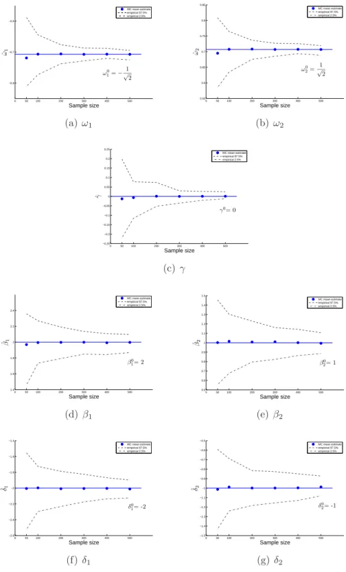
For change-line regression, in contrast, we assume that two subgroups have regres-sion models with different regresregres-sion parameters β and δ, respectively, whereβ0 ≠_δ0_, such that

E(Y;θ)=C(X;ω, γ)βTZ+{1−C(X;ω, γ)}δTZ, (3.3) where C(X)=1{ωT_X₋_γ >₀}_, _θ=(_{ζ, ϕ})_, _ϕ=(_{ω, γ})_{, and} _ζ =(_β

1, . . . , βp, δ1, . . . , δp).

In change-line regression, we estimate θ through least squares, which is the same as finding the M-estimator that maximizes Mn(θ)=nPnmθ where

Mn(θ)=− n

∑

i=1[

yi−C(xi;ω, γ)βTzi−{1−C(xi;ω, γ)}δTzi]

2

.

As before, let ˆθn be the maximizer of Mn(θ), where ˆθn ≡ (ζ,ˆ ϕˆ), ˆϕ = (ω,ˆ ˆγ), and

ˆ

ζ=(βˆ1, . . . ,βˆp, δˆ1, . . . ,δˆp).

3.1.2 Estimating procedure

In the present setting, the estimates are obtained in a similar way as done in Kosorok and Song [2007]. Before we begin estimation, we need to construct a set S(ω, γ)=

{(ω1, γ1), . . . ,(ωk, γk), k≤n(n−1)}, consisting of all possible lines generated by two

points (xi, xj) in R2 from n observations. In this thesis, S(ω, γ) is obtained by use

of the new algorithm developed by Kosorok [2008a], and described in Chapter 2.1.6. We search for γ by considering as candidates only elements of the set {γ1, . . . , γn−1} consisting of the midpoints of the sorted values of ωT_x

1, . . . , ωTxn.

The M-estimator ˆθn can be obtained in two steps. In the first step, for each fixed

(ω, γ) in S(ω, γ), we maximize the objective function Mn over model parameters

ζ to obtain the profile objective function pMn(ω, γ) ≡ sup ζ

Mn(ω, γ, ζ). In the

sec-ond step, (ωˆn,γˆn) can be obtained by searching for arg max

S(ω,γ)

(51)

search on the unit-circle for direction vector ω and on the line for a cut point γ. Let ˆζn = arg max

ζ

Mn(ζ,ωˆn,γˆn). By this procedure, we can obtain ˆθn = (ζ,ˆ γˆ) that

maximizes the objective function. Estimates for the model parameter obtained in this way are √n−consistent, and the estimate for the change-point parameters are

n−consistent. Also, this is an adaptive estimation procedure in the sense that we can have √n−consistent estimates for the model parameters whether or not we know the true value of the change-point parameter. We will show this in Chapter 4. Please see Pons [2003] and Kosorok and Song [2007] for similar results for the change-point model.

3.2 Simulation study

3.2.1 Change-line methods for heterogeneous subgroups

Two sets of simulation studies based on the Monte Carlo (MC) method were con-ducted to illustrate the applicability of the change-line classification and regression method.

Change-line classification model

The experimental data for the change-line classification model (3.2) were generated from the bivariate normal distribution with mean vector (µ0, µ1)T and covariance matrix Σ=diag(σ2

0, σ12). For all these simulations, the true values of the parameters were chosen as (ω0

1, ω20)=(−1/ √

2, 1/√2),γ0 =_0,(_µ0 0, σ

2,0

0 )=(2,4), (µ01, σ 2,0

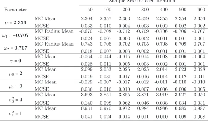
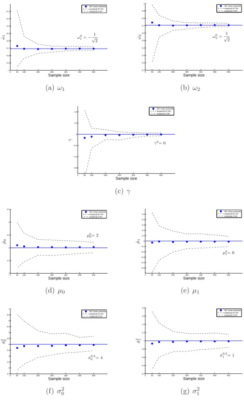
1 )=(0,1), and n0 = n1 = n/2. For a given sample size, 100 independently replicated samples were generated from the true model. Figure 3.1 and Table 3.1 display the results of simulations based on 100 replicated samples, with sample size ranging from 50 to 600. MC mean, MC standard error of estimates (MCSE), and 95% empirical

(52)

percentiles were calculated based on the 100 runs of simulations for each sample size. MC mean was calculated by θ¯ˆn =

100 ∑

j=1 ˆ

θn(j)/100, and MCSE was calculated by

¿ Á Á Á

À∑100j=1(θˆ( j)

n −(θ¯ˆn))2

100×(100−1) , where ˆθ

(j)

n denotes the estimate of the parameter θ from the

jth _{set of data,} _j = ₁_{, . . . ,}_{100. The MC radius mean for} (_ω

1, ω2) was calculated as (cos ¯û,sin ¯û), where û is estimate of the angle between the line ˆωT_X _{and the} _X_-axis.

Our method worked very well even for small sample sizes, and the MC mean of the estimates were close to the true values with smaller MCSE as sample size increased for both model parameters and change-line parameters.

To check the existence of an underlying change in the distribution ofY, a graphic examination was performed by displaying the Gaussian kernel estimates of the mean and standard deviation of Y. The Gaussian kernel estimates for the mean and stan-dard deviation were calculated by

ˆ

µ(y∣u) =

1

nh∑ n

i=1K(u−hui)yi

1

nh∑ n

i=1K(u−hui)

ˆ

σ(y∣u) =

¿ Á Á Ành1 ∑

n

i=1K(u−hui)(yi−µˆ(y∣u))2

1

nh∑ n

i=1K(u−hui)

,

where ui =ωˆTxi, i=1, . . . , n=600, K denotes the Gaussian kernel function, and h is

the bandwidth. We used the MC radius mean from the sample of size 600 for ˆω. Then we regressed the Gaussian kernel mean and standard deviation above onu by Robust Locally Weighted Least Squares Scatterplot Smoothing and a 1st _{degree polynomial}

(53)

Table 3.1: Summary statistics from 100 replications of simulation study for the change-line classification under various sample sizes : (50,100,200,300,400,500,600). For all simulations, true values of the parameter were chosen as (ω0

1 =

−1/√2, ω0₂ =1/√2, γ0 =₀_{, µ}0

0 =2, µ01=0, σ 2,0 0 =4, σ

2,0 1 =1).

Sample Size for each iteration

Parameter 50 100 200 300 400 500 600

MC Mean 2.304 2.357 2.363 2.359 2.355 2.354 2.356

α₌2.356

MCSE 0.033 0.010 0.004 0.003 0.002 0.002 0.002 MC Radius Mean -0.670 -0.708 -0.712 -0.709 -0.706 -0.706 -0.707

ω₁_{= −}0.707

MCSE 0.024 0.007 0.003 0.002 0.001 0.001 0.001 MC Radius Mean 0.743 0.706 0.702 0.705 0.708 0.709 0.707

ω₂ ₌0.707

MCSE 0.018 0.007 0.003 0.002 0.001 0.001 0.001 MC Mean -0.064 -0.044 -0.015 -0.014 -0.008 -0.006 -0.004

γ₌0

MCSE 0.028 0.011 0.005 0.003 0.002 0.001 0.001 MC Mean 2.099 2.053 2.026 2.025 2.014 2.023 2.028

µ₀₌2

MCSE 0.049 0.030 0.017 0.016 0.014 0.012 0.011 MC Mean -0.029 -0.007 -0.017 -0.012 -0.011 -0.010 -0.010

µ1=0

MCSE 0.036 0.016 0.010 0.007 0.006 0.006 0.005 MC Mean 3.693 3.851 3.855 3.871 3.919 3.927 3.950

σ₀2₌4

MCSE 0.140 0.098 0.062 0.046 0.038 0.034 0.031 MC Mean 0.931 0.970 0.972 0.984 0.986 0.985 0.987

σ₁2₌1

MCSE 0.041 0.024 0.014 0.011 0.010 0.009 0.008

5455.pdf

New statistical learning methods for chemical

toxicity data analysis

Abstract

Acknowledgments

Table of Contents

List of Figures

List of Tables

Chapter 1

Introduction

1.1

The change-line method

1.2

The interactive decision method

1.3

Outline of thesis

Chapter 2

Background

2.1

Change-line method

2.1.1

Projection pursuit regression

2.1.2

Latent classification/Latent class regression

2.1.3

Subgroup analysis in machine learning

2.1.4

Resampling or subsampling methods

2.1.5

Change-point analysis

2.1.6

Split-line algorithm

2.2

The interactive decision committee method

2.2.1

Literature review of the decision committee method

2.2.2

Background of method

2.3

Chemical toxicity data analysis

Chapter 3

The change-line classification and

regression method

3.1

Model and method

3.1.1

Data set-up and assumptions

3.1.2

Estimating procedure

3.2

Simulation study

3.2.1

Change-line methods for heterogeneous subgroups