CAHN-HILLIARD PHASE-FIELD MODEL BASED ON THE INVARIANT ENERGY QUADRATIZATION METHOD
XIAOFENG YANG∗, JIA ZHAO†, QI WANG‡, ANDJIE SHEN§
Abstract. How to develop efficient numerical schemes while preserving the energy stability at the discrete level is a challenging issue for the three component Cahn-Hilliard phase-field model. In this paper, we develop first and second order temporal approximation schemes based on the “Invariant Energy Quadratization” approach, where all nonlinear terms are treated semi-explicitly. Consequently, the resulting numerical schemes lead to a well-posed linear system with the symmetric positive definite operator to be solved at each time step. We rigorously prove that the proposed schemes are unconditionally energy stable. Various 2D and 3D numerical simulations are presented to demonstrate the stability and the accuracy of the schemes.
Key words. Phase-field; Chan-Hilliard; Three phase; Unconditional Energy Stability; Invariant Energy Quadrati-zation; Linear.
1. Introduction. The phase-field (i.e. the diffuse-interface) method is a robust modeling ap-proach to simulate the free interface problem (cf. [1,9,11,19,22,25,26,26,27,31,32,35,56,60,61,65,67,68], and the references therein). Its essential idea is to use one (or more) continuous phase-field variable(s) to describe different phases in the multi-components system (usually immiscible), and represents the interfaces by thin, smooth transition layers. The constitutive equations for those phase-field variables can be derived from the energetic variational formalism, the governing system of equations is thereby well-posed and thermo-dynamically consistent. Consequently, one can carry out mathematical analy-ses to obtain the existence and uniqueness of solutions in appropriate functional spaces, and to develop convergent numerical schemes.
For an immiscible, two phase system, the commonly used free energy for the system consists of (i) a double-well bulk part which promotes either of the two phases in the bulk, yielding a hydrophobic contribution to the free energy; and (ii) a conformational capillary entropic term that promotes hydrophilic property in the multiphase material system. The competition between the hydrophilic and hydrophobic part in the free energy enforces the coexistence of two distinctive phases in the immiscible two-phase system. The corresponding binary system can be modeled either by the Allen– Cahn equation (second order) or the Cahn–Hilliard equation (fourth order). For both of these models, there have been many theoretical analysis, algorithm developments and numerical simulations available in literatures (cf. [1,22,25,32]).
The generalization from the two-phase system to multi-phases have been studied by many works (cf. [2,3,5–7,14,15,20,21,28–30,38]). Specifically, for the system with three components, the general framework is to adopt three independent phase variables (c1, c2, c3) while imposing a hyperplane link condition among the three variables (c1+c2+c3 = 1). The bulk part of the free energy is simply a summation of the original double-well energy for each phase variable [6,7,27]. Moreover, in order to ensure the boundedness (from below) of the free energy, especially for the total spreading case
∗Corresponding author, Department of Mathematics, University of South Carolina, Columbia, SC 29208, USA.
Email: [email protected]. This author’s research is partially supported by the U.S. National Science Foundation under grant numbers DMS-1200487 and DMS-1418898.
†Department of Mathematics, University of North Carolina at Chapel Hill, Chapel Hill, NC, 27599, USA. Email: [email protected].
‡Department of Mathematics, University of South Carolina, Columbia, SC 29208; Beijing Computational Science
Re-search Center, Beijing, China; School of Mathematics, Nankai University, Tianjin, China; Email: [email protected]. This author’s research is partially supported by grants of the U.S. National Science Foundation under grant number DMS-1200487 and DMS-1517347, and a grant from the National Science Foundation of China under the grant number NSFC-11571032.
§Department of Mathematics, Purdue University, West Lafayette, IN 47906; Email:[email protected]. This
author’s research is partially supported by the U.S. National Science Foundation under grants 1419053, DMS-1620262 and AFOSR grant FA9550-16-1-0102.
1
where some coefficients of the bulk energy become negative, an extra sixth order polynomial term is needed [6,7], which couples the three phase variables altogether.
It is challenging to develop efficient schemes while preserving the energy stability to solve the three component Cahn-Hilliard phase-field system, since all three phase variables are nonlinearly coupled. Although a variety of numerical algorithms have been developed for it, most of the existing methods are either first-order accurate in time, or energy unstable, or highly nonlinear, or even the combinations of these features. We refer to [7] for a summary on recent advances about the three-phase models and their numerical approximations. For the developments of numerical methods, we emphasize that the preservation of energy stability laws is critical to capture the correct long time dynamics of the system especially for the preassigned grid size and time step. Furthermore, the energy-law preserving schemes provide flexibility for dealing with stiffness issue in phase-filed models. For the binary phase field model, it is well known that the simple fully implicit or explicit type schemes will induce quite severe stability conditions on the time step so they are not efficient in practice (cf. [17,18,43,44,52]). Such phenomena appear in the computations of the three component Cahn-Hilliard model as well (cf. the numerical examples in [7]). In particular, the authors of [7] concluded that (i) the fully implicit discretization of the six-order polynomial term leads to convergence of the Newton linearization method only under very tiny time step practically; (ii) it is an open problem about how to prove the existence and convergence of the numerical solutions for the fully implicit type scheme theoretically for the total spreading case; (iii) it is questionable to establish convex-concave decomposition for the six order polynomial term; and (iv) the semi-implicit scheme is the best choice that the authors in [7] can obtain since it is unconditionally energy stable for arbitrary time step, and the existence and the convergence can be thereby proved. However, the semi-implicit schemes referred in [7] are nonlinear, thus they require some efficient iterative solvers in the implementations.
The focus of this paper is to develop stable (unconditionally energy stability) and more efficient (linear) schemes to solve the three component Cahn-Hilliard system. Instead of using traditional dis-cretization approaches like simple implicit, stabilized explicit, convex splitting, or other various tricky Taylor expansions to discretize the nonlinear potentials, we adopt the Invariant Energy Quadratiza-tion(IEQ) approach, that has been successfully applied in the context of other models in the authors’ other work (cf. [23,54,58,59,62,70]). However, the application of IEQ method to the three compo-nent model is faced with new challenges due to the particular nonlinearities including the Lagrange multiplier term, and the sixth order polynomial potential. The essential idea of the IEQ method is to transform the free energy into a quadratic form of a new variable via a change of variables since the nonlinear potential is usually bounded from below. The new, equivalent system still retains a similar energy dissipation law in terms of new variables. For the time-continuous case, the energy law of the new reformulated system is equivalent to the energy law of the original system. A great advantage of such a reformulation is that all nonlinear terms can be treated semi-explicitly, which in turn leads to a linear system. Moreover, the resulting linear system is symmetric positive definite, thus it can be solved efficiently with simple iterative methods such as CG or other Krylov subspace methods. Using this new strategy, we develop a series of linear and energy stable numerical schemes, without introducing artificial stabilizers as in [43,52] or using convex splitting approach (cf. [10,16,50,51]).
In summary, the new numerical schemes that we develop in this paper possess the following properties: (i) the schemes areaccurate(ready for second order or even higher order in time); (ii) they areunconditionally energy stable; and (iii) they areefficient and easy to implement(lead to symmetric positive definite linear system at each time step). To the best of our knowledge, the proposed schemes are the first such schemes for solving the three-phase Cahn-Hilliard phase-field system that can have all these desired properties. In addition, when the three component Cahn-Hilliard model is coupled with the hydrodynamics (Navier-Stokes), the proposed schemes can be easily applied without any essential difficulties.
case. In Section 4, we present various 2D and 3D numerical simulations to validate the accuracy and efficiency of the proposed schemes. Finally, some concluding remarks are presented in Section 5.
2. Model System. We now introduce the three component Cahn-Hilliard phase-field model proposed in [6,7]. Let Ω be a smooth, open bounded, connected domain in Rd, d = 2,3. Let c
i (i= 1,2,3) be thei−thphase function (or order parameter) which represents the volume fraction of thei−th component in the fluid mixture, i.e.,
(2.1) ci=
(
1 inside the i-th component,
0 outside the i-th component.
In the phase-field framework, a thin (of thickness) but smooth layer is used to connect the interface that is between 0 and 1. The three unknownsc1, c2, c3are linked though the relationship:
c1+c2+c3= 1. (2.2)
This is the link condition for the vectorC= (c1, c2, c3), where it belongs to the hyperplane
S={C= (c1, c2, c3)∈R3, c1+c2+c3= 1}. (2.3)
In the two-phase model, the free energy of the mixture is as follows,
Ediph(c) = Z
Ω 3
4σ|∇c| 2+ 12σ
c
2(1−c)2dx, (2.4)
whereσis the surface tension parameter, the first term contributes to the hydrophilic type (tendency of mixing) of interactions between the materials and the second part, the double well bulk energy term represents the hydrophobic type (tendency of separation) of interactions. As the consequence of the competition between the two types of interactions, the equilibrium configuration will include a diffusive interface with thickness proportional to the parameter; and, asapproaches zero, we expect to recover the sharp interface separating the two different materials (cf., for instance, [8,13,64]).
There exist several generalizations from the two-phase model to the three-phase model (cf. [6,7, 29]). In this paper, we adopt below the approach in [7], where the free energy is defined as:
Etriph(c
1, c2, c3) = Z
Ω 3
8Σ1|∇c1| 2+3
8Σ2|∇c2| 2+3
8Σ3|∇c3| 2+12
F(c1, c2, c3)
dx,
(2.5)
where the coefficient of entropic terms Σi can be negative for some specific situations.
To be algebraically consistent with the two-phase systems, the three surface tension parameters
σ12, σ13, σ23should verify the following conditions:
Σi=σij+σik−σjk, i= 1,2,3. (2.6)
The nonlinear potential F(c1, c2, c3) is:
F(c1, c2, c3) =σ12c21c22+σ13c21c23+σ23c22c23+c1c2c3(Σ1c1+ Σ2c2+ Σ3c3) + 3Λc21c22c23. (2.7)
Sincec1, c2, c3 satisfy the hyperplane link condition (2.2), the free energy can be rewritten as
where
F0(c1, c2, c3) = Σ1 2 c
2
1(1−c1)2+Σ2 2 c
2
2(1−c2)2+Σ3 2 c
2
3(1−c3)2,
P(c1, c2, c3) = 3Λc21c22c23, (2.9)
and Λ is a non negative constant.
Therefore, the time evolution ofciis governed by the gradient of the energy Etriph with respect to theH−1(Ω) gradient flow, namely, the Cahn-Hilliard type dynamics as
cit= M0 Σi∆µi, (2.10)
µi=−3
4Σi∆ci+ 12
∂iF+β, i= 1,2,3,
(2.11)
with the initial condition
ci|(t=0)=c0i, i= 1,2,3, c01+c02+c03= 1, (2.12)
whereβ is the Lagrange multiplier to ensure the hyperplane link condition (2.2), that can be derived as
β=−4ΣT ( 1 Σ1∂1F+
1 Σ2∂2F+
1 Σ3∂3F), (2.13)
with
3 ΣT =
1 Σ1
+ 1 Σ2
+ 1 Σ3
.
(2.14)
We consider in this paper either of the two type boundary conditions below:
(i) all variables are periodic,or (ii)∂nci|∂Ω=∇µi·n|∂Ω= 0, i= 1,2,3, (2.15)
wheren is the unit outward normal on the boundary∂Ω.
It is easily seen that the three chemical potentials (µ1, µ2, µ3) are linked through the relation
µ1 Σ1 +
µ2 Σ2+
µ3 Σ3 = 0. (2.16)
Remark2.1. In the physical literatures, the coefficient Σi is called the spreading coefficient of the phase i at the interface between phases j and k. Since Σi is determined by the surface tensions σi,j, it might not be always positive. If Σi>0, the spreading is said to be “partial”, and ifΣi<0, it
is called “total”.
The following lemmas hold (cf. [6]):
Lemma2.1. There existsΣ>0 such that
Σ1|ξ1|2+ Σ1|ξ1|2+ Σ1|ξ1|2≥Σ
|ξ1|2+|ξ2|2+|ξ3|2
,∀ξ1+ξ2+ξ3= 0, (2.17)
if and only if the following condition holds:
Σ1Σ2+ Σ1Σ3+ Σ2Σ3>0,Σi+ Σj>0,∀i6=j. (2.18)
For any Λ>0, the bulk free energy F(c1, c2, c3)defined in (2.8)is bounded from below ifc1, c2, c3 is
on the hyperplane S in 2D. Furthermore, the lower bound only depends onΣ1,Σ2,Σ3 andΛ.
Remark2.2. From Lemma2.1, when (2.18)holds, the summation of the gradient entropy term is bounded from below since ∇(c1+c2+c3) = 0, i.e.,
Σ1k∇c1k2+ Σ2k∇c2k2+ Σ3k∇c3k2≥Σ(k∇c1k2+k∇c2k2+k∇c3k2)≥0. (2.19)
Remark2.3. The bulk part energyF(c1, c2, c3)defined in (2.8)has to be bounded from below in
order to form a meaningful physical system. For partial spreading case (Σi>0∀i), one can drop the six order polynomial term by assuming Λ = 0 since F0(c1, c2, c3) ≥0 is naturally satisfied. For the
total spreading case, Λhas to be non zero. Moreover, to ensure the non-negativity forF,Λhas to be large enough.
For 3D case, it is shown in [6] that the bulk energy F is bounded from below whenP(c1, c2, c3)
takes the following form:
P(c1, c2, c3) = 3Λc21c22c32(φα(c1) +φα(c2) +φα(c3)) (2.20)
whereφα(x) = (1+1x2)α with0< α≤ 178.
Since (2.9) is commonly used in literatures (cf. [6,7]), we adopt it as well for convenience. Nonetheless, it will be clear that the numerical schemes we develop in this paper can deal with ei-ther (2.9)or (2.20)without any difficulties.
Remark2.4. The system (2.10)-(2.11)is equivalent to the following system with two order pa-rameters,
cit= M0 Σi∆µi,
µi=−3
4Σi∆ci+ 12
∂iF+β, i= 1,2, c3= 1−c1−c2,
µ3 Σ3 =−(
µ1 Σ1+
µ2 Σ2). (2.21)
We omit the detailed proof since it is quite similar to Theorem 3.1in section 3.
The model equation (2.10)-(2.11) follows the dissipative energy law. More precisely, by taking theL2inner product of (2.10) with−µi, and of (2.11) withcit, and perform integration by parts, we obtain
−(cit, µi) =
M0 Σi k∇µik
2, (2.22)
(µi, cit) = 3
4Σi(∇ci, ∂t∇ci) + 12
(∂iF, cit) + (β, cit).
(2.23)
Taking summation of the two equalities fori= 1,2,3, and notice that (β,(c1+c2+c3)t) = (β,(1)t) = 0, we obtain the energy dissipative law as
d dtE
triph(c
1, c2, c3) =−M0 1
Σ1k∇µ1k 2+ 1
Σ2k∇µ2k 2+ 1
Σ3k∇µ3k 2. (2.24)
Since (µ1, µ2, µ3) satisfies the condition (2.16), if (2.18) holds, we can derive
−M0 1
Σ1k∇µ1k 2+ 1
Σ2k∇µ2k 2+ 1
Σ3k∇µ3k 2
≤ −M0Σ(k∇µ1k 2
Σ2 1
+k∇µ2k 2
Σ2 2
+ k∇µ3k 2
Σ2 3
)≤0.
3. Numerical schemes. We develop in this section several first and second order, uncondition-ally energy stable and linear numerical schemes for solving the three component phase-field model (2.10)-(2.11). To this end, the main challenges are how to discretize the following three terms includ-ing (i) the nonlinear term associated with the double well potential F0, (ii) the six order polynomial termP, (iii) the Lagrange multiplier termβ, especially when some Σi<0 (total spreading).
We notice that for the two-phase Cahn-Hilliard model, the discretization of the nonlinear, cubic polynomial term induced from the double well potential had been well studied (cf. [27,32,34,37, 49]). In summary, there are two commonly used techniques to discretize it in order to preserve the unconditional energy stability. The first is the so-called convex splitting approach [16,23,24,40,71,72], where the convex part of the potential is treated implicitly and the concave part is treated explicitly. The convex splitting approach is energy stable, however, it produces nonlinear schemes, thus the implementations are often complicated with potentially high computational costs.
The second technique is the so-called stabilization approach [9,33,36,41–43,45–48,52,53,55,57, 63,66,69], where the nonlinear term is treated explicitly. In order to preserve the energy law, a linear stabilizing term has to be added, and the magnitude of that term usually depends on the upper bound of the second order derivative of the G-L potential. The stabilized approach leads purely linear schemes, thus it is easy to implement and solve. However, it appears that second order schemes based on the stabilization are only conditionally energy stability [43]. On the other hand, the nonlinear potential may not satisfy the condition required for the stabilization. A feasible remedy is to make some reasonable revisions to the nonlinear potential in order to obtain a finite bound, for example, the quadratic order cut-off functions for the double well potential (cf. [43,52]). Such method is particularly reliable for those models with maximum principle. If the maximum principle does not hold, modified nonlinear potentials may lead to spurious solutions.
For the three component Cahn-Hilliard model system, the above two approaches cannot be easily applied. First of all, even though the convex-concave decomposition can be applied to F0, it is not clear how to deal with the sixth order polynomial term [7]. Second, it is uncertain whether the solution of the system satisfies certain maximum principle so the condition required for stabilization is not satisfied. Third, unconditional energy stable schemes are hardly obtained for both approaches if second order schemes are considered.
We aim to develop numerical schemes that are efficient (well-posed linear system), stable (uncon-ditionally energy stable), and accurate (ready for second order or even higher order in time). To this end, we use the IEQ approach, without worrying about whether the continuous/discrete maximum principle holds or a convexity/concavity splitting exists.
3.1. Transformed system. Since F(c1, c2, c3) is always bounded from below from Lemma2.2 for 2D and Remark 2.3for 3D. Therefore, we can rewrite the free energy functional F(c1, c2, c3) to the following equivalent form
F(c1, c2, c3) = (F(c1, c2, c3) +B)−B, (3.1)
whereBis some constant to ensureF(c1, c2, c3)+B >0. Furthermore, we define an auxiliary function as follows,
U =pF(c1, c2, c3) +B. (3.2)
In turn, the total free energy (2.5) can be rewritten as
Etriph(c
1, c2, c3, U) = Z
Ω 3
8Σ1|∇c1| 2+3
8Σ2|∇c2| 2+3
8Σ3|∇c3| 2+12
U
2dx− 12
B|Ω|,
(3.3)
cit= M0 Σi∆µi, (3.4)
µi=−3
4Σi∆ci+ 24
HiU+β, i= 1,2,3,
(3.5)
Ut =H1c1t+H2c2t+H3c3t, (3.6)
where
H1= δU
δc1 = 1 2
Σ1 2 (c1−c
2
1)(1−2c1) + 6Λc1c22c23 p
F(c1, c2, c3) +B
,
(3.7)
H2= δU
δc2 = 1 2
Σ2
2 (c2−c22)(1−2c2) + 6Λc21c2c23 p
F(c1, c2, c3) +B
,
(3.8)
H3= δU
δc3 = 1 2
Σ3
2 (c3−c23)(1−2c3) + 6Λc21c22c3 p
F(c1, c2, c3) +B
,
(3.9)
β=−8ΣT( 1 Σ1
H1+ 1 Σ2
H2+ 1 Σ3
H3)U. (3.10)
The transformed system (3.4)–(3.6) in the variablesc1, c2, c3, U form a closed PDE system with the following initial conditions,
ci(t= 0) =c0i, i= 1,2,3,
U(t= 0) =U0= q
F(c0
1, c02, c03) +B. (3.11)
Since the equations (3.6) for the new variablesU is only ordinary differential equation with time, the boundary conditions of the new system (3.4)-(3.6) are still (2.15).
Remark3.1. The system (3.4)-(3.6)is equivalent to the following two order parameter system
cit= M0 Σi∆µi,
µi=−3
4Σi∆ci+ 24
HiU+β, i= 1,2, Ut=H1c1t+H2c2t+H3c3t,
(3.12)
with
c3= 1−c1−c2,
µ3 Σ3
=−(µ1 Σ1
+ µ2 Σ2
).
(3.13)
Since the proof is quite similar to Theorem3.1, we omit the proof here.
We can easily obtain the energy law for the new system (3.4)-(3.6). Taking theL2 inner product of (3.4) with −µi, of (3.5) with∂tci, of (3.6) with−24U, taking the summation fori= 1,2,3, and noticing that (β, ∂t(c1+c2+c3)) = 0 from Remark3.1, we still obtain the energy dissipation law as
d dtE
triph(c
1, c2, c3, U) =−M0 1
Σ1k∇
µ1k2+ 1 Σ2k∇
µ2k2+ 1 Σ3k∇
µ3k2
≤ −M0Σ(k∇µ1k 2
Σ2 1
+ k∇µ2k 2
Σ2 2
+k∇µ3k 2
Σ2 3
)≤0.
Remark3.2. The new transformed system(3.4)-(3.6)is equivalent to the original system(2.10)
-(2.11)since (3.2)can be obtained by integrating (3.6)with respect to the time. Therefore, the energy law (3.14) for the transformed system is exactly the same as the energy law (2.24) for the original system.
We emphasize that we will develop energy stable numerical schemes for the new transformed system (3.4)- (3.6). The proposed schemes will follow a discrete energy law corresponding to (3.14)
instead of the energy law for the original system (2.24).
Letδt >0 denote the time step size and set tn =n δt for 0 ≤n≤ N with T = N δt. We also denote by (f(x), g(x)) = RΩf(x)g(x)dxthe L2 inner product of any two functions f(x) andg(x), and bykfk=p(f, f) theL2 norm of the functionf(x).
3.2. First order scheme. We now present the first order time stepping scheme to solve the system (3.4)-(3.6) where the time derivative is discretized based on the first order backward Euler method.
Assuming that (c1, c2, c3, U)n are already calculated, we compute (c1, c2, c3, U)n+1from the fol-lowing temporal discrete system:
cni+1−cni
δt =
M0 Σi ∆µ
n+1 i , (3.15)
µni+1=− 3 4Σi∆c
n+1
i +
24
H
n
iUn+1+βn+1, i= 1,2,3, (3.16)
Un+1−Un=H1n(cn1+1−cn1) +H2n(cn2+1−cn2) +H3n(cn3+1−cn3), (3.17)
where
H1n= 1 2
Σ1
2 (cn1−cn12)(1−2cn1) + 6Λcn1cn22cn32 p
F(cn
1, cn2, cn3) +B
,
(3.18)
H2n= 1 2
Σ2
2 (cn2−cn22)(1−2cn2) + 6Λcn12cn2cn32 p
F(cn
1, cn2, cn3) +B
,
(3.19)
Hn 3 =
1 2
Σ3
2 (cn3−cn32)(1−2cn3) + 6Λcn12cn22cn3 p
F(cn
1, cn2, cn3) +B
,
(3.20)
βn+1=−8
ΣT(
1 Σ1H
n 1 +
1 Σ2H
n 2 +
1 Σ3H
n 3)Un+1. (3.21)
The initial conditions are (3.11), and the boundary conditions are
(i) all variables are periodic,or (ii)∂ncni+1|∂Ω=∇µin+1·n|∂Ω= 0, i= 1,2,3. (3.22)
We immediately derive the following result which ensures the numerical solutions satisfy the hyperplane condition (2.2).
Theorem 3.1. The system of (3.15)-(3.17)is equivalent to the following scheme with two order
parameters,
cni+1−cni
δt =
M0 Σi ∆µ
n+1 i , (3.23)
µni+1=− 3 4Σ1∆c
n+1
i +
24
H
n
iUn+1+βn+1, i= 1,2, (3.24)
Un+1−Un=Hn
with
cn3+1= 1−cn1+1−cn2+1, (3.26)
µn3+1 Σ3 =−(
µn1+1 Σ1 +
µn2+1 Σ2 ). (3.27)
Proof. From (3.21), we can easily show that the following indentity holds,
24
( Hn
1 Σ1
+H n 2 Σ2
+H n 3 Σ3
)Un+1+βn+1( 1 Σ1
+ 1 Σ2
+ 1 Σ3
) = 0.
(3.28)
• (i) We first assume that (3.23)-(3.27) are satisfied, and derive (3.15)-(3.16). By taking the summation of (3.23) fori= 1,2, and applying (3.26) and (3.27), we obtain
cn3+1−cn 3
δt =
M0 Σ3
∆µn3+1. (3.29)
From (3.28), (3.24), (3.26) and (3.27), we obtain
µn3+1=−Σ3(µ n+1 1 Σ1 +
µn2+1 Σ2 )
=−Σ3
−34∆cn1+1− 3 4∆c
n+1
2 +
24
( Hn
1 Σ1
+H n 2 Σ2
)Un+1+βn+1( 1 Σ1
+ 1 Σ2
)
= 3 4Σ3∆c
n+1
3 +
24
H
n
3Un+1+βn+1. (3.30)
• (ii) We then assume that (3.15)-(3.16) are satisfied, and derive (3.23)-(3.27). By taking the summation of (3.15) fori= 1,2,3, we derive
Sn+1−Sn
δt =M0∆Θ
n+1, (3.31)
whereSn=cn
1+cn2+cn3 and Θn+1= Σ11 µ n+1 1 + Σ21µ
n+1 2 +Σ31µ
n+1
3 . From (3.16) and (3.28), we derive
Θn+1=−34∆Sn+1.
(3.32)
By taking theL2inner product of (3.31) with−Θn+1, of (3.32) withSn+1−Sn, and taking the summation of the two equalities above, we derive
3 8(k∇S
n+1k2− k∇Snk2+k∇Sn+1− ∇Snk2) +δtM
0k∇Θn+1k2= 0. (3.33)
SinceSn= 1, the lefthand side of (3.33) is a sum of non negative terms, thus∇Sn+1= 0, and
∇Θn+1= 0, i.e., the functionsSn+1and Θn+1are constants. Then (3.32) leads to Θn+1= 0, and (3.31) leads to Sn+1= Sn = 1. Thus we obtain (3.26). By dividing Σi for (3.16) and taking the summation of it fori= 1,2,3, and applying (3.28) and (3.26), we obtain (3.27).
The most impressing part of the above scheme if we notice that the nonlinear coefficientHiof the new variableU are treated explicitly, which can tremendously speed up the computations in practice. Moreover, we can rewrite the equations (3.17) as follows:
Un+1=Hn
whereQn
1 =Un−H1ncn1−H2ncn2−H3ncn3. Thus, the system (3.15)- (3.17) can be rewritten as
cni+1−cni
δt =
M0 Σi ∆µ
n+1 i , (3.35)
µni+1=− 3 4Σi∆c
n+1
i +
24
H
n
i(H1ncn1+1+H2ncn2+1+H3ncn3+1) (3.36)
+βn+1+24
H
n
iQn1, i= 1,2,3,
Theorem 3.2. Assuming (2.18), the linear system (3.35)-(3.36)for the variableΦ= (cn1+1,cn2+1,
cn3+1)T is symmetric (self-adjoint) and positive definite.
Proof. Taking theL2inner product of (3.35) with 1, we derive Z
Ω
cni+1dx= Z
Ω
cnidx=· · ·= Z
Ω
c0idx. (3.37)
Letα0 i = |Ω1|
R
Ωc0idx,γ0i = |Ω1| R
Ωµ n+1
i dx, and define
b
cni+1=cni+1−α0
i,µbni+1=µ n+1 i −γi0. (3.38)
Thus, from (3.35)-(3.36), (bcni+1,µbni+1) are the solutions for the following equations with unknowns (Ci, µi),
Ci
M0δt − 1 Σi∆µi=
b
cn i
M0δt, (3.39)
µi+γi0=− 3
4Σi∆Ci+ 24
H
n
iP1n+1+βn+1+gin, (3.40)
whereP1n+1=H1nC1+H2nC2+H3nC3 and
C1+C2+C3= 0, Z
Ω
Cidx= 0, Z
Ω
µidx= 0. (3.41)
We define the inverse Laplace operatoru(withRΩudx= 0)→v:= ∆−1u by
∆v=u,
Z
Ω
vdx= 0,
with the boundary conditions either (i)vis periodic,or (ii)∂nv|∂Ω= 0 (3.42)
Applying−∆−1 to (3.39) and using (3.40), we obtain
− Σi
M0δt∆ −1C
i−3
4Σi∆Ci+ 24
H
n
iP1n+1+βn+1−γ0i =−Σi∆−1 b
cn i
M0δt−g n
i, i= 1,2,3. (3.43)
We express the above linear system (3.43) asAC=b, whereC= (C1, C2, C3)T.
For any Φ = (φ1, φ2, φ3)T,Ψ = (ψ1, ψ2, ψ3)T with P3i=1φi = P3i=1ψi = 0 and RΩφidx = R
Ωψidx= 0, we can easily derive
(AΦ,Ψ) = (Φ,AΨ),
thusAis self-adjoint. Meanwhile, we have
(AΦ,Φ) = 1
M0δt(Σ1(−∆ −1φ
1, φ1) + Σ2(−∆−1φ2, φ2) + Σ3(−∆−1φ3, φ3))
+3
8(Σ1k∇φ1k 2+ Σ
2k∇φ2k2+ Σ3k∇φ3k2) +24
kH
n
1φ1+H2nφ2+H3nφ3k2 (3.45)
Letdi= ∆−1φi, i.e.,
∆di=φi, Z
Ω
didx= 0, (3.46)
with periodic boundary conditions or∂ndi|∂Ω= 0. Therefore, we have
(−∆−1φi, φi) =k∇dik2. (3.47)
Furthermore,Z=d1+d2+d3 satisfies
∆Z= 0,
Z
Ω
Zdx= 0,
(3.48)
with periodic boundary conditions or∂nZ|∂Ω= 0. ThusZ=d1+d2+d3= 0. From (2.19), we derive
(AΦ,Φ)≥M1
0δtΣ(k∇d1k 2+
k∇d2k2+k∇d3k2) + 3
8Σ(k∇φ1k 2+
k∇φ2k2+k∇φ3k2)
+ 24
kH
n
1φ1+H2nφ2+H3nφ3k2≥0, (3.49)
and (AΦ,Φ) = 0 if and only if Φ = 0. Thus we conclude the theorem.
Remark3.3. We can show the well-posedness of the linear systemAC=bfrom the Lax-Milgram theorem noticing that the linear operator Ais bounded and coercive inH1(Ω). We leave the detailed
proof to the interested readers since the proof is rather standard.
The stability result of the first order scheme (3.15)-(3.17) is given below.
Theorem 3.3. When (2.18)holds, the first order linear scheme (3.15)-(3.17)is unconditionally
energy stable, i.e., satisfies the following discrete energy dissipation law:
1
δt(E
n+1
1st −E1nst)≤ −M0Σ
k∇µn+1 1 k2 Σ2
1
+k∇µ n+1 2 k2 Σ2
2
+ k∇µ n+1 3 k2 Σ2
3
.
(3.50)
whereEn
1st is defined by
E1nst= 3 8Σ1k∇c
n 1k2+
3
8Σ2k∇c n 2k2+
3
8Σ3k∇c n 3k2+
12
kU
n
k2−12 B|Ω|.
(3.51)
Proof. Taking theL2inner product of (3.15) with−δtµn+1
i , we obtain
−(cni+1−cni, µni+1) =δt
M0 Σik∇µ
n+1 i k2. (3.52)
Taking theL2inner product of (3.16) withcn+1
i −cni and applying the following identities
we derive
(µni+1, cni+1−cni) = 3
8Σi(k∇c n+1
i k2− k∇cnik2+k∇cni+1− ∇cnik2)
+24
(H
n
i Un+1, cni+1−cni) + (βn+1, cni+1−cni). (3.54)
Taking theL2inner product of (3.17) with 24
Un+1, we obtain
12
kUn+1k2− kUnk2+kUn+1−Unk2
= 24
Hn
1(cn1+1−cn1), Un+1
+ Hn
2(cn2+1−cn2), Un+1
+ Hn
3(cn3+1−cn3), Un+1
.
(3.55)
Combining (3.52), (3.54), taking the summation fori= 1,2,3 and using (3.55) and (3.26), we have
3 8
3 X
i=1
Σik∇cni+1k2− k∇cnik2
+3 8
3 X
i=1
Σik∇cni+1− ∇cnik2
+12
kUn+1k2− kUnk2=−M 0( 1
Σ1k∇µ n+1 1 k2+
1 Σ2k∇µ
n+1 2 k2+
1 Σ3k∇µ
n+1 3 k2)
≤ −M0Σ(k∇µn1+1k2+k∇µ2n+1k2+k∇µn3+1k2)≤0. (3.56)
Noticing thatP3i=1∇(cni+1−cni) = 0, we derive
3 X
i=1
Σik∇cni+1− ∇cnik2
≥Σ 3 X
i=1
k∇cni+1− ∇cnik2
≥0.
(3.57)
Therefore, the desired result (3.50) is obtained.
Remark3.4. We remark that the discrete energy E1st defined in (3.51) is bounded from below.
Such property is particularly significant. Otherwise, the energy stability does not make any sense. The essential idea of the IEQ method is to transform the complicated nonlinear potentials into a simple quadratic form in terms set of some new variables via a change of variables. Such a simple way of quadratization provides some great advantages. First, the complicated nonlinear potential is transferred to a quadratic polynomial form that is much easier to handle. Second, the derivative of the quadratic polynomial is linear, which provides the fundamental support for linearization method. Third, the quadratic formulation in terms of new variables can automatically keep this property of positivity (or bounded from below) of the nonlinear potentials.
We must notice that the convexity is required in the convex splitting approach [16]; and the bound-edness for the second order derivative is required in the stabilization approach [43,52]. Compared with those two methods, the IEQ method provides much more flexibilities to treat the complicated nonlinear terms since the only request of it is that the nonlinear potential has to be bounded from below.
Meanwhile, the choices of new variables are not unique. For instance, for the partial spreading case where Σi>0, ∀i, we can define four functions Ub1,Ub2,Ub3, V as follows,
b
Ui=ci(1−ci), i= 1,2,3,
Thus the free energy becomes
E(Ub1,Ub2,Ub3, V) = Z
Ω 3
8Σ1|∇c1| 2+ 3
8Σ2|∇c2| 2+ 3
8Σ3|∇c3| 2
+12
Σ1 2 Ub
2 1 +
Σ2 2 Ub
2 2+
Σ3 2 Ub
2
3+ 3ΛV2
dx.
(3.59)
For this new definition of the free energy, one can carry about the similar analysis. The details are left to the interested readers.
However, we notice this particular transformation only works for the partial spreading case. For the total spreading case, since for some i, Σi <0, the energy defined in (3.59)may not be bounded from below. This is the particular reason that we define the new variable U in (3.2)in this paper.
As can be seen in this paper, the IEQ approach is able to provide enough flexibilities to derive the equivalent PDE system, and hence the corresponding numerical schemes with unconditional energy stabilities.
Remark3.5. The proposed scheme follows the new energy dissipation law (3.14)instead of the energy law for the originated system (2.24). For time-continuous case, (3.14)and (2.24)are identical. For time-discrete case, the discrete energy law (3.50)is the first order approximation to the new energy law (3.14). Moreover, the discrete energy functional E1nst+1 is also the first order approximation to
E(φn+1)(defined in(2.5)), sinceUn+1is the first order approximations toqF(cn+1
1 , cn2+1, cn3+1) +B,
that can be observed from the following facts, heuristically. We rewrite (3.17)as follows,
Un+1−
q
F(cn1+1, cn2+1, cn3+1) +B=Un− q
F(cn
1, cn2, cn3) +B+Rn+1, (3.60)
whereRn+1=O(P3i=1(c n+1
i −cni)2).
Since Rk = O(δt2)for 0≤ k≤n+ 1 and U0 = p
F(c0
1, c02, c03) +B, by mathematical induction
we can easily get
Un+1= q
F(cn1+1, cn2+1, c3n+1) +B+O(δt). (3.61)
3.3. Second order scheme based on Crank-Nicolson. We now present a second order time stepping scheme to solve the system (3.4)-(3.6).
Assumming that (c1, c2, c3, U)n and (c1, c2, c3, U)n−1 are already calculated, we compute (c1,c2,
c3,U)n+1 from the following temporal discrete system
cit=
M0 Σi ∆µ
n+1 2 i , (3.62)
µn+12
i =−
3 4Σi∆
cni+1+cni
2 +
24
H
∗ iUn+
1 2 +βn+
1
2, i= 1,2,3, (3.63)
Un+1−Un=H∗
where
Un+1 2 = U
n+1+Un
2 ,
c∗i = 3 2c n i − 1 2c
n−1 i ,
H1∗= 1 2
Σ1
2 (c∗1−c∗12)(1−2c∗1) + 6Λc∗1c∗22c∗32 p
F(c∗
1, c∗2, c∗3) +B
,
H2∗= 1 2
Σ2
2 (c∗2−c∗22)(1−2c∗2) + 6Λc∗12c∗2c∗32 p
F(c∗
1, c∗2, c∗3) +B
,
H3∗= 1 2
Σ3
2 (c∗3−c∗32)(1−2c∗3) + 6Λc∗12c∗22c∗3 p
F(c∗1, c∗2, c∗3) +B
,
βn+12 =−8
ΣT(
1 Σ1
H1∗+ 1 Σ2
H2∗+ 1 Σ3
H3∗)Un+ 1 2. (3.65)
The initial conditions are (3.11), and the boundary conditions are
(i) all variables are periodic,or (ii)∂ncni+1|∂Ω =∇µn+ 1 2
i ·n|∂Ω= 0, i= 1,2,3. (3.66)
The following theorem ensures the numerical solution (cn1+1, cn2+1, cn3+1) always satisfies the hy-perplane link condition (2.2).
Theorem 3.4. The system (3.62)-(3.64) is equivalent to the following scheme with two order
parameters,
cni+1−cni
δt =
M0 Σi∆µ
n+1 2 i , (3.67)
µn+12
i =−
3 4Σi∆
cni+1+cni
2 +
24
H
∗ iUn+
1
2 +βn+12, i= 1,2, (3.68)
with
cn3+1= 1−cn1+1−cn2+1, (3.69)
µn+12 3 Σ3
=−(µ n+1
2 1 Σ1
+ µ n+1
2 2 Σ2
).
(3.70)
Proof. The proof is omitted here since it is similar to that for Theorem3.1.
Similar to the first orders scheme, we can rewrite the system (3.64) as follows,
Un+1=H1∗c1n+1+H2∗c2n+1+H3∗cn3+1+Qn2, (3.71)
whereQn
2 =Un−H1∗cn1−H2∗cn2−H3∗cn3. Thus, the system (3.62)- (3.64) can be rewritten as
cni+1−cni
δt =
M0 Σi ∆µ
n+1 2 i , (3.72)
µn+12
i =−
3 4Σi∆
cni+1+cni
2 +
24
H
∗
i(H1∗cn1+1+H2∗cn2+1+H3∗cn3+1) (3.73)
+βn+12+ 24
H
∗
Theorem 3.5. The linear system (3.72)-(3.73) for the variable Φ = (c1n+1, cn2+1, cn3+1)T is
self-adjoint and positive definite.
Proof. The proof is omitted here since it is similar to that for Theorem3.2.
The stability result of the second order Crank-Nicolson scheme (3.62)-(3.64) is given below.
Theorem 3.6. Assuming (2.18), the second order Crank-Nicolson scheme (3.62)-(3.64)is
uncon-ditionally energy stable and satisfies the following discrete energy dissipation law:
1
δt(E
n+1
cn −Ecnn) =−M0
1
Σ1k∇µ n+1
2 1 k2+
1 Σ2k∇µ
n+1 2 2 k2+
1 Σ3k∇µ
n+1 2 3 k2
≤ −M0Σ
k∇µn+1 2 1 k2 Σ2
1
+ k∇µ n+1
2 2 k2 Σ2
2
+k∇µ n+1
2 3 k2 Σ2
3
,
(3.74)
whereEn
cn that is defined by
En cn =
3 8Σ1k∇c
n 1k2+
3
8Σ2k∇c n 2k2+
3
8Σ3k∇c n 3k2+
12
kU
nk2−12
B|Ω|.
(3.75)
Proof. Taking theL2inner product of (3.62) with−δtµn+1
i , we obtain
−(cni+1−cni, µ n+1
2 i ) =δt
M0 Σik∇µ
n+1 2 i k2. (3.76)
Taking theL2inner product of (3.63) withcn+1
i −cni, we obtain
(µn+12 i , c
n+1 i −c
n i) =
3
8Σi(k∇c n+1 i k
2
− k∇cnik2)
+24
(H
∗ iUn+
1 2, cn+1
i −c n
i) + (βn+ 1 2, cn+1
i −c n i). (3.77)
Taking theL2inner product of (3.17) with 24 Un+
1
2, we obtain
24
(H1∗(c1n+1−cn1), Un+ 1
2) + (H∗
2(cn2+1−cn2), Un+ 1
2) + (H∗
3(cn3+1−cn3), Un+ 1 2)
= 12
(kU
n+1k2− kUnk2) (3.78)
Combining (3.76), (3.77) fori= 1,2,3 and (3.78), we derive
3 8
3 X
i=1
Σik∇cni+1k2− k∇cnik2
+12
kUn+1k2− kUnk2
=−M0( 1 Σ1k∇µ
n+1 2 1 k2+
1 Σ1k∇µ
n+1 2 1 k2+
1 Σ1k∇µ
n+1 2 1 k2)
≤ −M0Σ0(k∇µ n+1
2 1 k2 Σ2
1
+k∇µ n+1
2 2 k2 Σ2
2
+ k∇µ n+1
2 3 k2 Σ2
3 ).
(3.79)
Thus we obtain the desired result (3.74).
Remark3.6. We remark that the energy law for the second order Crank-Nicolson scheme is “=” instead of “≤” (the first equality in (3.74)).
Assumming that (c1, c2, c3, U)n and (c1, c2, c3, U)n−1 are already calculated, we compute (c1,c2,
c3,U)n+1 from the following discrete system:
3cni+1−4cn i +cni−1
2δt =
M0 Σi∆µ
n+1 i , (3.80)
µni+1=−34Σ1∆cni+1+ 24
H
†
iUn+1+βn+1, i= 1,2,3, (3.81)
3Un+1−4Un+Un−1=H1†(3cn1+1−4cn1+cn1−1) (3.82)
+H2†(3cn2+1−4cn2+cn2−1) +H3†(3cn3+1−4cn3 +cn3−1),
where
c†i = 2cni −cni−1
H1†= 1 2
Σ1
2 (c†1−c†1 2
)(1−2c†1) + 6Λc†1c†2 2
c†3 2
q
F(c†1, c†2, c†3) +B
H2†= 1 2
Σ2
2 (c†2−c†2 2
)(1−2c†2) + 6Λc†1 2
c†2c†3 2
q
F(c†1, c†2, c†3) +B
H3†= 1 2
Σ3 2 (c
† 3−c†3
2
)(1−2c†3) + 6Λc1†2c†22c†3
q
F(c†1, c†2, c†3) +B
βn+1=−8
ΣT(
1 Σ1
H1†+ 1 Σ2
H2†+ 1 Σ3
H3†)Un+1. (3.83)
The initial conditions are (3.11), and the boundary conditions are
(i) all variables are periodic,or (ii)∂ncni+1|∂Ω=∇µin+1·n|∂Ω= 0, i= 1,2,3. (3.84)
Similar to the first order scheme and the second order Crank-Nicolson scheme, the hyperplane link condition still holds for this scheme.
Theorem 3.7. The system (3.80)-(3.82) is equivalent to the following scheme with two order
parameters,
3cni+1−4cni +cni−1
2δt =
M0 Σi∆µ
n+1 i , (3.85)
µni+1=− 3 4Σi∆c
n+1
i +
24
H
†
iUn+1+βn+1, i= 1,2, (3.86)
cn3+1= 1−cn1+1−cn2+1,
(3.87)
µn3+1 Σ3 =−(
µn1+1 Σ1 +
µn2+1 Σ2 ). (3.88)
Proof. The proof is omitted here since it is similar to that for Theorem3.1.
Similar to the two previous schemes, we can rewrite the sysytem (3.82) as
Un+1=H1†c1n+1+H2†c2n+1+H3†cn3+1+Qn3, (3.89)
whereQn
3 =U −H1†c1 −H2†c2 −H3†c3 and V = 4V
n
−Vn−1
(3.80)- (3.82) can be rewritten as
3cni+1−4cni +cni−1
2δt =
M0 Σi∆µ
n+1 i , (3.90)
µni+1=− 3 4Σi∆c
n+1
i +
24
H
†
i(H1†cn1+1+H2†cn2+1+H3†cn3+1) (3.91)
+βn+1+24
H
†
iQn3, i= 1,2,3,
Theorem 3.8. The linear system (3.90)-(3.91) for the variable Φ = (c1n+1, cn2+1, cn3+1)T is
self-adjoint and positive definite.
Proof. The proof is omitted here since it is similar to that for Theorem3.2.
Theorem 3.9. The second order scheme (3.80)-(3.82)is unconditionally energy stable and
satis-fies the following discrete energy dissipation law:
1
δt(E
n+1 bdf −E
n
bdf)≤ −M0 1
Σ1k∇µ n+1 1 k2+
1 Σ2k∇µ
n+1 2 k2+
1 Σ3k∇µ
n+1 3 k2
≤ −M0Σ
k∇µn+1 1 k2 Σ2
1
+k∇µ n+1 2 k2 Σ2
2
+ k∇µ n+1 3 k2 Σ2
3
,
(3.92)
whereEn
bdf is defined by
Enbdf= 3 8Σ1
k∇cn 1k2
2 +
k2∇cn
1− ∇cn1−1k2 2
+3
8Σ2 k∇cn
2k2
2 +
k2∇cn
2− ∇cn2−1k2 2
+3 8Σ3
k∇cn 3k2
2 +
k2∇cn
3− ∇cn3−1k2 2
+ 12
kUnk2
2 +
k2Un−Un−1k2 2
−12
B|Ω|.
(3.93)
Proof. Taking theL2inner product of (3.80) with−2δtµn+1
i , we obtain
−(3cni+1−4cni +cni−1, µ n+1 i ) = 2δt
M0 Σik∇µ
n+1 i k
2. (3.94)
Taking theL2inner product of (3.80) with 3cn+1
i −4cni+cni−1, and applying the following identities the following identity
2(3a−4b+c, a) =|a|2− |b|2+|2a−b|2− |2b−c|2+|a−2b+c|2, (3.95)
we derive
(µni+1,3cni+1−4cni +cni−1) = 3 8Σi
k∇cni+1k2− k∇cnik2+k2∇cin+1− ∇cnik2− k2∇cni − ∇cni−1k2
+ 3 8Σik∇c
n+1
i −2∇cni +∇cni−1k2
+ 24
(H
†
Taking theL2inner product of (3.82) with 24
Un+1, we obtain
12
kUn+1k2− kUnk2+k2Un+1−Unk2− k2Un−Un−1k2+kUn+1−2Un+Un−1k2
= 24
(H1†(3cn1+1−4cn1+cn1−1), Un+1) + (H2†(3cn2+1−4c2n+cn2−1), Un+1)
+ (H3†(3cn3+1−4cn
3+cn3−1), Un+1)
.
(3.97)
Combining (3.76), (3.77) fori= 1,2,3 and (3.78), we derive
3 8
3 X
i=1
Σik∇cni+1k2+k2∇cni+1− ∇cnik2 −3 8 3 X i=1
Σik∇cnik2+k2∇cni − ∇cni−1k2 +3 8 3 X i=1
Σik∇cni+1−2∇cni +∇cni−1k 2+12
kUn+1k2+k2Un+1−Unk2
−12
kUnk2+k2Un−Un−1k2+ 12
kU
n+1−2Un+Un−1k2
=−2δtM0 1
Σ1k∇µ n+1 1 k2+
1 Σ2k∇µ
n+1 2 k2+
1 Σ3k∇µ
n+1 3 k2
≤ −2δtM0Σ
k∇µn+1 1 k2 Σ2
1
+ k∇µ n+1 2 k2 Σ2
2
+k∇µ n+1 3 k2 Σ2
3
.
(3.98)
SinceP3i=1(∇cni+1−2∇cni +∇cni−1) = 0, from Lemma2.1, we have
3 X
i=1 n
Σik∇cni+1−2∇cni +∇cni−1k2 o ≥Σ 3 X i=1 n
k∇cni+1−2∇cni +∇cni−1k2 o
≥0.
(3.99)
Therefore, we obtain (3.92) after we drop the unnecessary positive terms in (3.98).
Remark3.7. From formal Taylor expansion, we find
kφn+1k2+k2φn+1−φnk2 2δt
−kφ
nk2+k2φn−φn−1k2
2δt
∼ =kφ
n+2k2− kφnk2
2δt
+O(δt2)∼= d
dtkφ(t
n+1)k2+O(δt2), (3.100)
and
kφn+1−2φn+φn−1k2
δt ∼=O(δt
3) (3.101)
for any variable φ. Therefore, the discrete energy law (3.92) is a second order approximation of
d
dtEtriph(φ)in (3.14).
4. Numerical Simulations. We present in this section several 2D and 3D numerical experi-ments using the schemes constructed in the last section. The computational domain is Ω = (0,1)d, d= 2,3. We use the second order central finite difference method in space with 128d grid points in all simulations.
Unless otherwise explicitly specified, the default parameters are
Coarseδt Fineδt L2−Error Order L1−Error Order L∞−Error Order
0.01 0.005 7.120e-3 – 3.969e-1 – 3.950e-4 –
0.005 0.0025 3.816e-3 0.90 2.112e-1 0.91 2.067e-4 0.93
0.0025 0.00125 1.999e-3 0.93 1.101e-1 0.94 1.062e-4 0.96
0.00125 0.000625 1.028e-3 0.96 5.645e-2 0.96 5.395e-5 0.98
0.000625 0.0003125 5.225e-4 0.98 2.863e-2 0.98 2.719e-5 0.99
0.0003125 0.00015625 2.635e-4 0.99 1.442e-2 0.99 1.365e-5 0.99
0.00015625 0.000078125 1.323e-4 0.99 7.239e-3 0.99 6.842e-6 1.0
Table 4.1
TheL2, L1, L∞numerical errors att= 1that are computed by the first order scheme LS1 using various temporal
resolutions. The order parameters are of (4.1)and1282grid points are used to discretize the space.
Coarseδt Fineδt L2−Error Order L1−Error Order L∞−Error Order
0.01 0.005 3.636e-3 – 1.541e-1 – 2.460e-4 –
0.005 0.0025 1.205e-3 1.59 4.972e-2 1.63 9.311e-5 1.40
0.0025 0.00125 3.590e-4 1.75 1.453e-2 1.78 2.999e-5 1.63
0.00125 0.000625 9.936e-5 1.85 3.941e-3 1.88 8.653e-6 1.79
0.000625 0.0003125 2.626e-5 1.92 1.030e-3 1.93 2.336e-6 1.89
0.0003125 0.00015625 6.759e-6 1.96 2.636e-4 1.97 6.080e-7 1.94
0.00015625 0.000078125 1.715e-7 1.98 6.671e-5 1.98 1.551e-7 1.97
Table 4.2
TheL2, L1, L∞numerical errors att= 1that are computed by the second order scheme LS2-CN using various
temporal resolutions. The order parameters are of (4.1)and1282 grid points are used to discretize the space.
4.1. Accuracy test. For convenience, we denote the first order scheme (3.15)-(3.17) by LS1, the second order scheme (3.62)-(3.64) by LS2-CN, the scheme (3.80)-(3.82) by LS2-BDF.
We set the initial condition as follows,
φ3= 1
2(1 + tanh
R−0.15
),
φ1= 1
2(1−φ3)(1 + tanh
y−0.5
),
Coarseδt Fineδt L2−Error Order L1−Error Order L∞−Error Order
0.01 0.005 6.368e-3 – 5.374e-1 – 5.018e-4 –
0.005 0.0025 2.584e-3 1.30 2.143e-1 1.33 1.811e-4 1.47
0.0025 0.00125 9.528e-4 1.44 7.588e-2 1.50 5.836e-5 1.63
0.00125 0.000625 3.172e-4 1.59 2.443e-2 1.64 2.244e-5 1.38
0.000625 0.0003125 9.641e-5 1.72 7.488e-3 1.71 7.170e-6 1.65
0.0003125 0.00015625 2.626e-5 1.88 2.095e-3 1.84 1.955e-6 1.87
0.00015625 0.000078125 7.012e-6 1.91 6.424e-4 1.70 5.099e-7 1.94
Table 4.3
TheL2, L1, L∞numerical errors att= 1that are computed by the second scheme LS2-BDF using various temporal
resolutions. The order parameters are of (4.1)and1282grid points are used to discretize the space.
Fig. 4.1. Theoretical shape of the contact lens at the equilibrium between two stratified fluid components [6].
whereR=p(x−0.5)2+ (y−0.5)2. Since the exact solutions are not known, we compute the errors by adjacent time step. We present the summations of the L2, L1 and L∞ errors of the three phase variables at t = 1 with different time step sizes in Table 4.1, 4.2 and 4.3 for the three proposed schemes. We observe that the schemes LS1, LS2-CN and LS2-BDF asymptotically match the first order and second order accuracy in time, respectively.
4.2. Liquid lens between two stratified fluids. Next, we perform simulations for the classical test case of a liquid lens that is initially spherical sitting at the interface between two other phases. For the accuracy reason, we always use the second order scheme LS2-CN and take the time step
δt= 0.001.
The equilibrium state in the limit→0 can be computed analytically: the final shape of the lens is the union of two pieces of circles, the contact angles being given as a function of the three surface tensions by the Young relations as shown in Fig. 4.1(cf. [6,27,39]).
sinθ1
σ23 = sinθ2
σ13 = sinθ3
σ12 . (4.3)
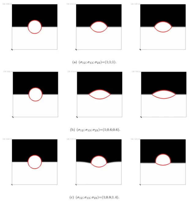
(a) (σ12;σ13;σ23)=(1;1;1).
(b) (σ12;σ13;σ23)=(1;0.6;0.6).
(c) (σ12;σ13;σ23)=(1;0.8;1.4).
Fig. 4.2. The dynamical behaviors until the steady state of a liquid lens between two stratified fluids for the partial spreading case, with three sets of different surface tension parameters σ12, σ13, σ23, where the time step isδt= 0.001
and1282grid points are used. The color in black (upper half ), white (lower half ) and red circle (lens) represent fluids
I, II, and III respectively.
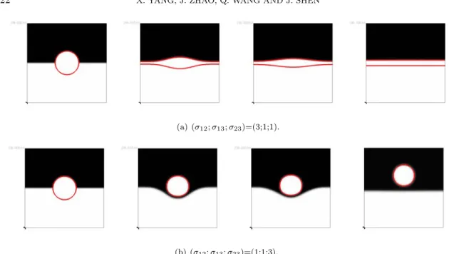
(a) (σ12;σ13;σ23)=(3;1;1).
(b) (σ12;σ13;σ23)=(1;1;3).
Fig. 4.3. The dynamical behaviors until the steady state of a liquid lens between two stratified fluids for the total spreading case (no junction points), with two sets of different surface tension parametersσ12, σ13, σ23, where the time
step isδt= 0.001and1282 grid points are used. The color in black (upper half ), white (lower half ) and red circle
(lens) represent fluids I, II, and III respectively.
angles at equilibrium becomeθ1< θ3< θ2, which is consistent to the formulation (4.3) as well. We then simulate the total spreading case (no junction point) in Fig. 4.3. We set the three surface tension parameters σ12= 3, σ13= 1, σ23= 1. From (4.3), the three contact angles can be computed as θ1 = θ2 = π and θ3 = 0, that can be observed in Fig. 4.3 (a), where the third fluid component
c3 totally spread to a layer. For the final case, we set σ12 = 1, σ13 = 1, σ23 = 3. By (4.3), it can be computed that the three contact angles at equilibrium are θ1 = 0, θ2 = θ3 =π, which indicates that the first and third fluid components c1, c3 are totally spread, andc2 stays inside the first fluid component, as shown in Fig. 4.3(b). We remark that all numerical results are qualitatively consistent with the computation results obtained in [6,29].
4.3. Spinodal decomposition in 2D. In this example, we study the phase separation behavior, the so-called the spinodal decomposition phenomenon. The process of the phase separation can be studied by considering a homogeneous binary mixture, which is quenched into the unstable part of its miscibility gap. In this case, the spinodal decomposition takes place, which manifests in the spontaneous growth of the concentration fluctuations that leads the system from the homogeneous to the two-phase state. Shortly after the phase separation starts, the domains of the binary components are formed and the interface between the two phases can be specified [4,12,73]. For the accuracy reason, we always use the second order scheme LS2-CN and take the time stepδt= 0.001.
The initial condition is taken as the randomly perturbed concentration fields as follows.
φi= 0.5 + 0.001rand(x, y), ci|(t=0)= φi
φ1+φ2+φ3
, i= 1,2,3,
(4.4)
where the rand(x, y) is the random number in [−1,1] and has zero mean. To label the three phases, we use pink, grey and yellow to represents phases I, II, and III respectively.
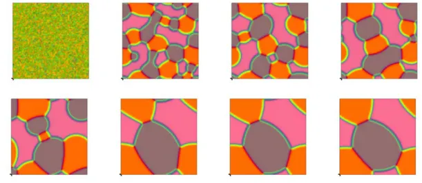
Fig. 4.4. The 2D dynamical evolution of the three phase variableci, i= 1,2,3for the partial spreading case, where order parameters are(σ12;σ13;σ23) = (1 : 1 : 1), the time step isδt= 0.001and1282 grid points are used. Snapshots
of the numerical approximation are taken att= 0,1000,2000,5000,10000,20000,25000,30000. The color in pink , grey and yellow represents the three phases I, II, and III respectively.
Fig. 4.5. The 2D dynamical evolution of the three phase variables ci, i= 1,2,3 for the partial spreading case, where the order parameters are(σ12;σ13;σ23) = (1,0.8,1.4), the time step isδt= 0.001and1282grid points are used.
Snapshots of the numerical approximation are taken att= 0,1000,2000,5000,10000,20000,25000,30000. The color in pink , grey and yellow represents the three phases I, II, and III respectively.
presents a very regular shape where the three contact angles areθ1=θ2=θ3= 23π. In Fig. 4.5, with the same initial condition, we set the surface tension parameters are σ12 = 1, σ13 = 0.8, σ23 = 1.4. The final equilibrium solution aftert= 30000 presents show three different contact angles that obey
θ1 < θ3< θ2 which is consistent to the example Fig. 4.2(c). The total spreading case is simulated in Fig. 4.6, in which we set the surface tension parameters areσ12= 1, σ13= 1, σ23 = 3. The final equilibrium solution aftert= 30000 presents that no junction points appear, similar as Fig. 4.3(b).
Fig. 4.6. The 2D dynamical evolution of the three phase variable ci for the total spreading case (no junction points), where the order parameters are(σ12;σ13;σ23) = (1,1,3), the time step isδt= 0.001and1282grid points are
used. Snapshots of the numerical approximation are taken att = 0,1000,2000,5000,10000,20000, 25000,30000. The color in pink , grey and yellow represents the three phases I, II, and III respectively.
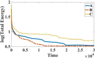
Fig. 4.7. Time evolution of the free energy functional using the algorithm LS2-CN usingδt= 0.001for the three order parameters set of A : (σ12;σ13;σ23) = (1,0.8,1.4) (partial spreading), B : (σ12;σ13;σ23) = (1,1,1)(partial
spreading), andC: (σ12;σ13;σ23) = (1,1,3)(total spreading). The x-axis is time, and y-axis islog10(total energy).
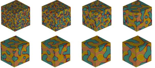
4.4. Spinodal decomposition in 3D. Finally, we present 3D simulations of the phase sepa-ration dynamics using the second order scheme LS2-CN and time step δt = 0.001. In order to be consistent with the 2D case, the initial condition reads as follows,
φ(t= 0) = 0.5 + 0.001rand(x, y, z),
(4.5)
where the rand(x, y, z) is the random number in [−1,1] with zero mean.
Fig. 4.8. The 3D dynamical evolution of the three phase variables ci, i= 1,2,3 for the partial spreading case, where the order parameters are(σ12;σ13;σ23) = (1 : 1 : 1)and time step isδt= 0.001. 1283 grid points are used to
discretize the space. Snapshots of the numerical approximation are taken att= 50,100,200,500,750,1000,1500,2000. The color in pink , grey and yellow represents the three phases I, II, and III respectively.
Fig. 4.9. The 3D dynamical evolution of the three phase variableci, i= 1,2,3for the partial spreading case, where the order parameters are (σ12;σ13;σ23) = (1 : 0.8 : 1.4)and time step is δt= 0.001. 1283 grid points are used to
discretize the space. Snapshots of the numerical approximation are taken att= 50,100,200,500,750,1000,1500,2000. The color in pink , grey and yellow represents the three phases I, II, and III respectively.
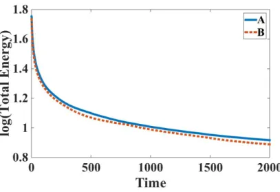
4.4. We observe that the three components accumulate, as shown in 2D case. In Fig. 4.9, we set the surface tension parametersσ12= 1, σ13= 0.8, σ23= 1.4, we observe that the three components accumulate but with different contact angles which is also consistent to the 2D case. In Fig. 4.10, we present the evolution of the free energy functional, in which the energy curves show the decays with time.
Fig. 4.10.Time evolution of the free energy functional using the algorithm LS2-CN usingδt= 0.001for the three order parameters set of A: (σ12;σ13;σ23) = (1,0.8,1.4)andB : (σ12;σ13;σ23) = (1,1,1). The x-axis is time, and
y-axis islog10(total energy).
convex splitting and the stabilized approach and enjoy the following desirable properties: (i)accurate
(up to second order in time); (ii)unconditionally energy stable; and (iii)easy to implement(one only solves linear equations at each time step). Moreover, the resulting linear system at each time step is symmetric, positive definite so that it can be efficiently solved by any Krylov subspace methods with suitable (e.g., block-diagonal) pre-conditioners.
To the best of our knowledge, these new schemes are the first schemes that are linear and un-conditionally energy stable for the three component Cahn-Hilliard phase-field model. These schemes can be applied to the hydro-dynamically coupled three phase model without essential difficulty. Al-though we considered only time discretization in this study, it is expected that similar results can be established for a large class of consistent finite-dimensional Galerkin approximations since the proofs are all based on a variational formulation with all test functions in the same space as the space of the trial functions.
REFERENCES
[1] D. M. Anderson, G. B. McFadden, and A. A. Wheeler. Diffuse-interface methods in fluid mechanics. 30:139–165, 1998.
[2] J. W. Barrett and J. F. Blowey. An improved error bound for a finite element approximation of a model for phase separation of a multi-component alloy.IMA J. Numer. Anal., 19:147168, 1999.
[3] J. W. Barrett, J. F. Blowey, and H. Garcke. On fully practical finite element approximations of degenerate cahn-hilliard systems.ESAIM: M2AN, 35:713748, 2001.
[4] K. Binder. Collective diffusion, nucleation and spinodal decomposition in polymer mixtures. J. Chem. Phys., 79:6387–6409, 1983.
[5] J. F. Blowey, M. I. M. Copetti, and C.M. Elliott. Numerical analysis of a model for phase separation of a multi-component alloy.IMA J. Numer. Anal., 16:111139, 1996.
[6] F. Boyer and C. Lapuerta. Study of a three component cahn-hilliard flow model. ESAIM: M2AN, 40:653687, 2006.
[7] F. Boyer and S. Minjeaud. Numerical schemes for a three component cahn-hilliard model. ESAIM: M2AN, 45:697738, 2011.
[8] G. Caginalp and X. Chen. Convergence of the phase field model to its sharp interface limits.Euro. Jnl of Applied Mathematics, 9:417–445, 1998.
[10] W. Chen, S. Conde, C. Wang, X. Wang, and S. Wise. A linear energy stable scheme for a thin film model without slope selection.Preprint, 2011.
[11] A. Christlieb, J. Jones, K. Promislow, B. Wetton, and M. Willoughby. High accuracy solutions to energy gradient flows from material science models.Journal of Computational Physics, 257:192–215, 2014.
[12] P. G. de Gennes. Dynamics of fluctuations and spinodal decomposition in polymer blends.J. Chem. Phys., 7:4756, 1980.
[13] K. R. Elder, M. Grant, N. Provatas, and J. M. Kosterlitz. Sharp interface limits of phase-field models.Phys. Rev. E., 64:021604, 2001.
[14] C. M. Elliott and H. Garcke. Diffusional phase transitions in multicomponent systems with a concentration dependent mobility matrix.Physica D, 109:242256, 1997.
[15] C. M. Elliott and S. Luckhaus. A generalised diffusion equation for phase separation of a multi-component mixture with interfacial free energy.IMA Preprint Series, 887:242256, 1991.
[16] D. J. Eyre. Unconditionally gradient stable time marching the Cahn-Hilliard equation. InComputational and mathematical models of microstructural evolution (San Francisco, CA, 1998), volume 529 ofMater. Res. Soc. Sympos. Proc., pages 39–46. MRS, 1998.
[17] X. Feng, Y. He, and C. Liu. Analysis of finite element approximations of a phase field model for two-phase fluids. Math. Comp., 76(258):539–571, 2007.
[18] X. Feng and A. Prol. Numerical analysis of the allen-cahn equation and approximation for mean curvature flows. Numer. Math., 94:33–65, 2003.
[19] M. G. Forest, Q. Wang, and X. Yang. Lcp droplet dispersions: a two-phase, diffuse-interface kinetic theory and global droplet defect predictions.Soft Matter, 8:9642–9660, 2012.
[20] H. Garcke, B. Nestler, and B. Stoth. A multiphase field concept: numerical simulations of moving phase boundaries and multiple junctions.SIAM J. Appl. Math., 60:295315, 2000.
[21] H. Garcke and B. Stinner. Second order phase field asymptotics for multi-component systems. Interface Free Boundaries, 8:131–157, 2006.
[22] M. E. Gurtin, D. Polignone, and J. Vi˜nals. Two-phase binary fluids and immiscible fluids described by an order parameter.Math. Models Methods Appl. Sci., 6(6):815–831, 1996.
[23] D. Han, A. Brylev, X. Yang, and Z. Tan. Numerical analysis of second order, fully discrete energy stable schemes for phase field models of two phase incompressible flows. in press, DOI:10.1007/s10915-016-0279-5, J. Sci. Comput., 2016.
[24] D. Han and X. Wang. A Second Order in Time, Uniquely Solvable, Unconditionally Stable Numerical Scheme for Cahn-Hilliard-Navier-Stokes Equation.J. Comput. Phys., 290:139–156, 2015.
[25] D. Jacqmin. Calculation of two-phase Navier-Stokes flows using phase-field modeling.J. Comput. Phys., 155(1):96– 127, 1999.
[26] M. Kapustina, D.Tsygakov, J. Zhao, J. Wessler, X. Yang, A. Chen, N. Roach, Q.Wang T. C. Elston, K. Jacobson, and M. G. Forest. Modeling the excess cell surface stored in a complex morphology of bleb-like protrusions. PLOS Comput. Bio., 12:e1004841, 2016.
[27] J. Kim. Phase-field models for multi-component fluid flows.Commun. Comput. Phys., 12(3):613–661, 2012. [28] J. Kim, K. Kang, and J. Lowengrub. Conservative multigrid methods for ternary cahn-hilliard systems.Commun.
Math. Sci., 2:53–77, 2004.
[29] J. Kim and J. Lowengrub. Phase field modeling and simulation of three-phase flows.Interfaces Free Boundaries, 7:435466, 2005.
[30] H. G. Lee and J. Kim. A second-order accurate non-linear difference scheme for the n-component cahn-hilliard system.Physica A, 387:47874799, 2008.
[31] T. S. Little, V. Mironov, A. Nagy-Mehesz, R. Markwald, Y. Sugi, S. M. Lessner, M. A.Sutton, X. Liu, Q. Wang, X. Yang, J. O. Blanchette, and M. Skiles. Engineering a 3d, biological construct: representative research in the south carolina project for organ biofabrication.Biofabrication, 3:030202, 2011.
[32] C. Liu and J. Shen. A phase field model for the mixture of two incompressible fluids and its approximation by a Fourier-spectral method.Physica D, 179(3-4):211–228, 2003.
[33] C. Liu, J. Shen, and X. Yang. Decoupled energy stable schemes for a phase-field model of two-phase incompressible flows with variable density.J. Sci. Comput., 62:601–622, 2015.
[34] J. Lowengrub, A. Ratz, and A. Voigt. Phase field modeling of the dynamics of multicomponent vesicles spinodal decomposition coarsening budding and fission.Physical Review E, 79(3), 2009.
[35] J. Lowengrub and L. Truskinovsky. Quasi-incompressible Cahn-Hilliard fluids and topological transitions.R. Soc. Lond. Proc. Ser. A Math. Phys. Eng. Sci., 454(1978):2617–2654, 1998.
[36] L. Ma, R. Chen, X. Yang, and H. Zhang. Numerical approximations for allen-cahn type phase field model of two-phase incompressible fluids with moving contact lines.Comm. Comput. Phys., 21:867–889, 2017. [37] C. Miehe, M. Hofacker, and F. Welschinger. A phase field model for rate-independent crack propagation:
Ro-bust algorithmic implementation based on operator splits. Computer Methods in Applied Mechanics and Engineering, 199:2765–2778, 2010.
[38] B. Nestler, H. Garcke, and B. Stinner. Multicomponent alloy solidification: Phase-field modeling and simulations. Phys. Rev. E, 71:041609, 2005.
[39] J. S. Rowlinson and B. Widom. Molecular theory of capillarity.Clarendon Press, 1982.
![Fig. 4.1. Theoretical shape of the contact lens at the equilibrium between two stratified fluid components [6].](https://thumb-us.123doks.com/thumbv2/123dok_us/8287822.2194681/20.892.285.583.516.705/fig-theoretical-shape-contact-equilibrium-stratified-fluid-components.webp)