DESIGN AND CONTROL OF SERVICE CENTERS
Nelson Lee
A dissertation submitted to the faculty of the University of North Carolina at Chapel Hill in partial fulfillment of the requirements for the degree of Doctor of
Philosophy in the Department of Statistics and Operations Research.
Chapel Hill 2013
Approved by: Vidyadhar Kulkarni Nilay Argon
Jasleen Kaur Shu Lu
c 2013 Nelson Lee
ABSTRACT
Nelson Lee: DESIGN AND CONTROL OF SERVICE CENTERS (Under the direction of Vidyadhar Kulkarni)
A service center is a facility with multiple heterogeneous servers providing special-ized service to multiple types of customers. Design and control problems of service centers arise in many practical applications such as cloud computing, data centers, health care facilities, call centers, etc. With the motivation of reducing energy con-sumption in data centers, this dissertation investigates the design and control prob-lems from three different perspectives that are applicable to the service centers in general.
The first study provides decision models to determine optimal static assignment and routing policies, explicitly taking into account the stochastic fluctuations of de-mand along with the autocorrelations and cross-correlations of the different traffic streams. We consider several possible performance measures and formulate the de-sign problem as a mixed integer nonlinear programming problem. We also develop an efficient heuristic algorithm to enhance scalability. We observe numerically that the optimal routing policy tries to combine the negatively correlated traffic streams, and separate the positively correlated traffic streams.
that results in solutions that satisfy the given performance requirements with min-imum energy consumption. We also evaluate our policy with actual data collected from the VCL at North Carolina State University.
ACKNOWLEDGEMENTS
Five years ago, I came to North Carolina without knowing any single person here. When I look back, I cannot believe how many new mentors and friends I have met along this wonderful five-year Ph.D. journey.
First of all, I would like to express my deepest gratitude to my advisor, Professor Vidyadhar Kulkarni, for his priceless guidance and persistent encouragement over the past four years, which made my dissertation research a truly joyful and rewarding journey. He intrigued me not only the knowledge but more importantly, the attitude toward research.
TABLE OF CONTENTS
LIST OF TABLES . . . ix
LIST OF FIGURES . . . x
1 INTRODUCTION . . . 1
1.1 Related Work . . . 4
1.1.1 Data Center . . . 5
1.1.2 Call Center and Contact Center . . . 7
1.1.3 Health Care System . . . 7
2 OPTIMAL STATIC ASSIGNMENT AND ROUTING POLICIES 9 2.1 Introduction . . . 9
2.1.1 Related Work . . . 10
2.2 Problem Formulation . . . 12
2.3 Analysis of the Queueing Model . . . 15
2.3.1 Stability . . . 15
2.3.2 The Queuing Time Process . . . 16
2.3.3 Expected Waiting Time . . . 18
2.3.4 Expected Queue Length . . . 18
2.4 Optimal Assignment and Routing Policies . . . 18
2.5 Diffusion Approximation . . . 20
2.6 Convex Quadratic Model . . . 29
2.7 Solution . . . 37
2.7.2 Numerical Example I . . . 40
2.7.3 Numerical Example II: Virtual Computing Laboratory . . . . 48
2.8 Acknowledgment . . . 52
3 ENERGY EFFICIENT VIRTUAL COMPUTING LABS . . . 54
3.1 Introduction . . . 54
3.2 Problem Formulation . . . 55
3.3 The Stochastic Model . . . 57
3.3.1 Dedicated Pool . . . 58
3.3.2 Flexible Pool . . . 60
3.3.3 Modified SIPP Approach . . . 61
3.4 Data . . . 63
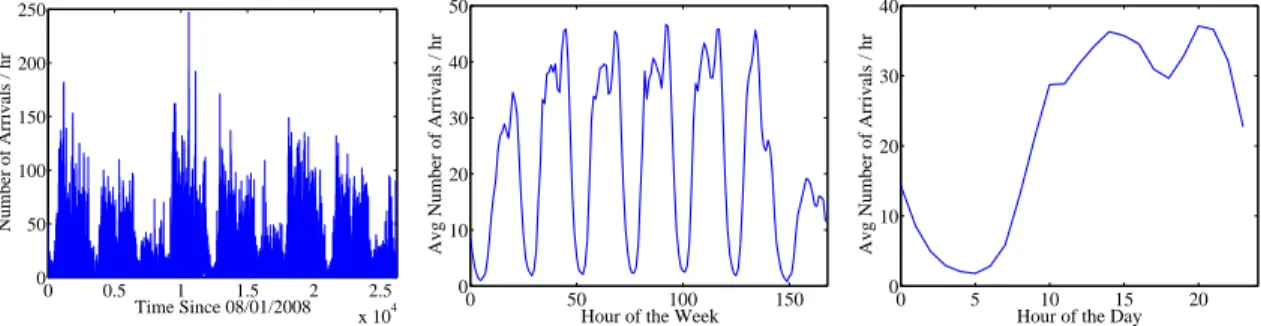
3.4.1 Arrival Data . . . 64
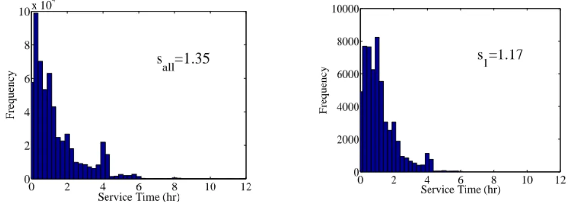
3.4.2 Service Time Data . . . 67
3.5 Simulation . . . 68
3.5.1 Synthetic Simulation . . . 68
3.5.2 Actual Data Simulation . . . 71
4 OPTIMAL ARRIVAL RATE AND SERVICE RATE CONTROL 76 4.1 Introduction . . . 76
4.2 Problem Formulation . . . 78
4.3 The Discounted Cost Optimal Policy . . . 80
4.4 The Average Cost Optimal Policy . . . 89
4.5 Service Rate Control with Batch Arrivals . . . 93
4.6 Acknowledgment . . . 94
5 CONCLUSIONS AND EXTENSIONS . . . 95
5.1 Conclusions . . . 95
LIST OF TABLES
2.1 Removal Progress Using Queueing Model . . . 44
2.2 Removal Progress Using Diffusion Approximation Model . . . 45
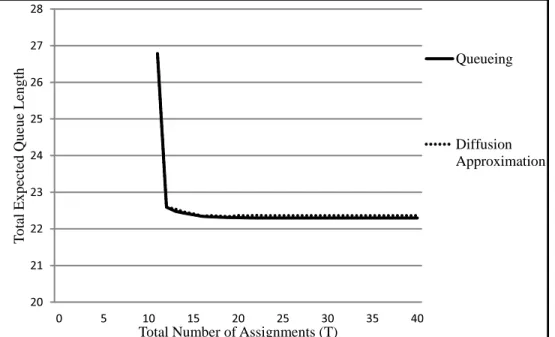
2.3 Example I: Total Expected Queue Length . . . 48
2.4 Example II: Total Expected Queue Length . . . 52
LIST OF FIGURES
2.1 Example I: Total Expected Queue Length . . . 48
2.2 Example II: Total Expected Queue Length . . . 53
3.1 Cumulative Relative Frequency of Arrivals . . . 65
3.2 Aggregated Arrivals (Overall) . . . 65
3.3 Aggregated Arrivals (Weekly Cycle) . . . 65
3.4 Aggregated Arrivals (Daily Cycle) . . . 65
3.5 Arrivals of Type 1 (Overall) . . . 66
3.6 Arrivals of Type 1 (Weekly Cycle) . . . 66
3.7 Arrivals of Type 1 (Daily Cycle) . . . 66
3.8 Arrivals of Type 10 (Overall) . . . 66
3.9 Arrivals of Type 10 (Weekly Cycle) . . . 66
3.10 Arrivals of Type 10 (Daily Cycle) . . . 66
3.11 Arrivals of Type 100 (Overall) . . . 66
3.12 Arrivals of Type 100 (Weekly Cycle) . . . 66
3.13 Arrivals of Type 100 (Daily Cycle) . . . 66
3.14 Service Times of All Application Sets . . . 67
3.15 Service Times of Application Set 1 . . . 67
3.16 Service Times of Application Set 10 . . . 67
3.17 Service Times of Application Set 100 . . . 67
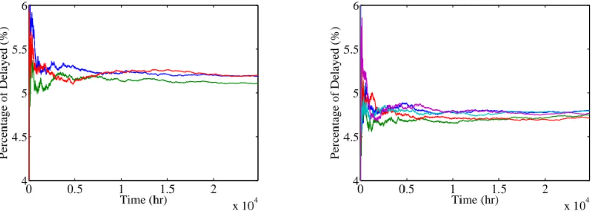
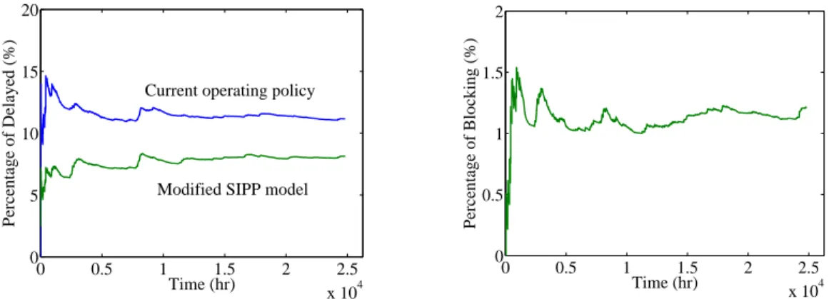
3.18 Percentage of Delayed (SIPP Model) . . . 69
3.19 Percentage of Delayed (Modified SIPP) . . . 69
3.20 Percentage of Blocking (SIPP Model) . . . 70
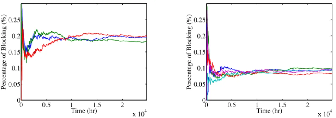
3.21 Percentage of Blocking (Modified SIPP) . . . 70
3.24 Percentage of Blocking (Modified SIPP) . . . 73
3.25 Number of Servers (Overall) . . . 74
3.26 Number of Servers (Weekly Cycle) . . . 74
CHAPTER 1: INTRODUCTION
A service center is a facility with multiple heterogeneous servers providing spe-cialized services to multiple types of customers. An incoming customer of each type requests a service requiring a random amount of time that may depend on customer type and/or server. The arrival processes of the incoming customers of different types form stochastic traffic streams that may be dependent on each other. The design and control problems of service centers of our interests include:
(1) Assignment: determine which server to enable to serve which set of customer types;
(2) Routing: determine which customer should be served by which server; (3) Sizing: determine the number of servers of each type;
(4) Scheduling: determine when to activate and de-activate servers;
(5) Rate control: determine the arrival rates of customers and the service rates of servers.
The objective of this kind of problems is usually to minimize the overall costs while fulfilling the requirements for quality of service, or to maximize appropriate system performance measure given the resource constraints.
centers are increasing rapidly these days. A modern data center usually consists of hundreds or thousands of servers. The energy consumption is becoming an important issue in large-scale computing environments, both economically and ecologically.
Although no official figures of server utilization in data centers are reported, it has been estimated that the common resource utilization is between 15 and 20 percents (Vogels [63]). The under-utilized servers result in hardware and energy wastage. With the motivation of reducing energy consumption in data centers, we investigate the design and control problems from three different perspectives that are applicable in more general settings. We consider the computers in data center as the servers in service center. A transaction request is an incoming customer of a certain type, who requires a specialized software application to serve. Transaction requests of each type form a traffic stream to the data center (service center).
In the past, organizations used to host most of their services on dedicated servers, i.e., each server could provide only one service. For example, payroll, inventory man-agement, and sales applications may be hosted on separate servers. A major reason to use dedicated servers is to avoid conflicts between services. However, dedicated servers most likely do not operate at their maximum capacities. They are usually expensive, under-utilized, and energy-consuming.
Nowadays, data center design and control have more flexibility due to technology improvements such as server virtualization and voltage control.
flexibility to run multiple isolated software application sets on a shared resource, and the benefit of server consolidation.
We investigate the benefit of server consolidation in service centers in Chapter 2, explicitly taking into account the stochastic fluctuations of demand along with the autocorrelations and cross-correlations of the different traffic streams. Most litera-ture in this area assumes independent traffic streams. In reality, the traffic streams usually have cycles and are correlated to each other, either positively or negatively. The service center performance can be further improved if we take these factors into consideration (Li [45]). We focus on Problems (1) and (2) together, and provide schemes to determine an optimal static assignment and routing policy with corre-lated traffic streams. Note that this study does not intend to minimize the system operating cost (energy consumption), but it has potential to be extended to further investigate how one can reduce the required number of servers while satisfying a given quality of service requirement by taking account the correlations between different traffic streams into design. We consider several possible performance measures and formulate the design problem as a mixed integer nonlinear programming problem. We also develop an efficient heuristic algorithm to enhance scalability, and compare the different policies using the heuristic algorithms. We observe numerically that the optimal routing policy tries to combine the negatively correlated traffic streams, and separate the positively correlated traffic streams.
may receive immediate service. However, this goal is unrealistic due to the large number of application sets. Using Erlang-B model, we provide a server scheduling and operating policy that results in solutions that satisfy the given performance requirements with minimum energy consumption. We also evaluate our policy with actual data collected from the VCL at North Carolina State University.
On modern servers, the frequencies of the processors, which determine the service rates, are usually controllable via voltage control. One usually observes a linear rela-tionship between service rates of servers and their processor frequencies, but a cubic relationship between power consumption of servers and their processor frequencies (Chen et al. [16], DVFS+DFS voltage and frequency scaling mechanism in Ghandi et al. [23]). This motivates us to look at Problem (5), and study the structural proper-ties of optimal arrival rate and service rates of multi-server queues in Chapter 4. The cost structure we consider includes customer holding cost which is a non-decreasing convex function of the number of customers in the system, server operating cost which is a non-decreasing convex function of the chosen service rate, and system op-erating reward which is a non-decreasing concave function of the chosen arrival rate. We formulate the problem as a continuous-time Markov decision process and derive structural properties of the optimal control policies under both discounted cost and average cost criterions. We show that the optimal arrival rate is non-increasing in the number of customers in the system, while the optimal service rate is non-decreasing in the number of customers in the system.
1.1
Related Work
design and control of queueing systems. Buzacott and Shanthikumar [15] focus on the design of queueing systems, and covers some of sizing, assignment, and routing problems that are of our interests. Stidham [58] also discusses design problems of queueing system from several aspects. However, none of these papers or the references therein consider the assignment and routing policies simultaneously with correlated arrival traffic as we do in Chapter 2.
Green, Kolesar, and Soares [28], and Green, Kolesar, and Whitt [29] discuss several scheduling problems of service centers with time-varying demands. Their methods mostly focus on the applications to service systems with human agents that are restricted with certain types of schedules. Unlike human agents, the computer systems considered in Chapter 3 may be ready for service in only a few minutes and it is relatively easy to change the number of servers. Hence, we propose a modification to their methods which takes advantage of real time information.
Sobel [55], Serfozo [51], Stidham and Weber [60], and Stidham [57] have reviewed most of the existing studies on the optimal control problems of queueing systems. Although Serfozo [51] and Anderson [4] have studied the optimal arrival rate and service rate control of a multi-server system, the cost structure we consider in Chapter 4, which is motivated by its application to data center operations, is different from those in their studies.
There are many other related papers on design and control of service centers with specific applications. We discuss some of most related ones in the following three separate subsections based on their applications.
1.1.1
Data Center
deter-ministic capacity demands for each customer type. They formulate the problem as a bin packing problem. Since the bin packing problem is NP-hard (Johnson et al. [37]), they introduce heuristic algorithms to solve the problem. However, these studies do not take into account the system performance requirements.
Chen et al. [16] consider a data center hosting multiple identical servers and providing multiple services. This paper assumes the servers can be turned on/off with adjustable service rates. The objective is to minimize the operating cost, in-cluding power consumption cost and setup cost, while satisfying average response time requirements. Anselmi, Amaldi, and Cremonesi [7] and Anselmi, Cremonesi, and Amaldi [8] consider multi-tiered services in the data centers. The objective is to minimize the number of servers used while satisfying performance requirements, such as end-to-end response time constraints and utilization constraints. Utiliza-tion constraints, similar to capacity demand constraints in Bichler et al. [12] and Speitkamp and Bichler [56], are linear, while end-to-end response time constraints are nonlinear. They assume each service tier can only be served by one server, and different application tiers can be served by a common server. They also consider load-balanced system, where traffic can be evenly split to multiple servers. Gandhi et al. [23] aim to minimize mean response time of a data center given total power consumption constraint assuming incoming traffic is evenly split to multiple servers. However, these papers do not address the issue of determining the routing policies as we do in Chapter 2 or the nonhomogeneous Poisson arrivals as we do in Chapter 3.
1.1.2
Call Center and Contact Center
Gans, Koole, and Mandelbaum [24] have a thorough discussion on the design and control of call centers. Wallace and Whitt [64] propose a staffing algorithm for call centers with performance constraints. Their paper states that the call centers can significantly decrease the number of servers if each agent has two skills instead of one. On the other hand, the additional benefit is not significant when the number of skills for each agent increases beyond two. They provide a heuristic algorithm and use simulation to solve the staffing problems. Their staffing algorithm is similar to our heuristic algorithm for finding the assignment policy in Chapter 2, but ours has a different type of routing policy involved.
Whitt [68], Harrison and Zeevi [34], and Bassamboo, Harrison, and Zeevi [11] approach call center problems by using multi-class stochastic fluid models. The ob-jective in these papers is to minimize the sum of staffing cost and expected aban-donment cost. Customer abanaban-donment plays a key role in their models. With fluid models, the problems or subproblems are formulated as linear programming prob-lems. However, the same framework may not be suitable for data center problems, because the overflow and customer abandonment are commonly seen in call centers but are less significant in data centers.
1.1.3
Health Care System
skill level is known. The objective is to minimize the labor costs while satisfying the demand. They further formulate the problem as a shortest path problem to improve the solution in order to satisfy human resource requirements such as workload, off weekends, and rotations.
CHAPTER 2: OPTIMAL STATIC ASSIGNMENT AND ROUTING POLICIES FOR SERVICE CENTERS WITH CORRELATED
TRAFFIC
2.1
Introduction
implementing dynamic policies accordingly involves a considerable communication overhead and typically nullifies the potential benefits of dynamic policies. Further-more, our optimal static routing policy will depend upon major system parameters, such as arrival rates, service rates, covariances between streams, etc. In practice, we may monitor these parameters continuously and adjust the optimal routing policy periodically to adapt the changes in these system parameters. We refer readers to Borst [14], Sethuraman and Squillante [52], Guo, Lu, and Squillante [30], and the references therein for deeper discussion of the motivation of static routing policy.
2.1.1
Related Work
Borst [14], Buzacott and Shanthikumar [15] (Section 6), and Sethuraman and Squillante [52] provide the structures of the optimal policy and frameworks for deter-mining an optimal routing policy with multiple classes of customers. Shanthikumar and Xu [53] and Guo, Lu, and Squillante [30] also have similar analysis on routing policies but with a single class of customer. Assuming a single class of customer and the service times are known upon arrivals, Harchol-Balter, Crovella, and Murta [33] compare several routing policies such as round-robin, random splitting, and join-the-shortest-queue. All the above mentioned papers mostly focus on optimal routing policies and assume either dedicated or fully flexible servers (i.e. each server can serve any type of customers). Gurvich, Armony, and Mandelbaum [31] and Gurvich and Whitt [32] study the sizing and routing problem of service system with multiple types of customers and servers, but the former paper assumes fully flexible servers and the latter one assumes the available assignments between type of customer and server are given. Thus none of these papers consider the assignment and routing policies simultaneously.
can postpone the routing decision until a server becomes free, if such a flexibility was possible. Several researchers have considered such a possibility. For example, Andrad´ottir, Ayhan, and Down [5, 6] and Tekin, Andrad´ottir, and Down [62] use the fluid model to determine maximum system capacity or throughput under dynamic server assignment policies and provide generalized round-robin policies that achieve the system capacity or throughput arbitrarily close to these upper bounds for queue-ing networks with flexible servers. However, they do not intend to optimize other system performance measures such as mean waiting time or queue length.
Moreover, most literature in this area assumes independent traffic streams. In reality, the traffic streams usually have cycles and are correlated to each other, either positively or negatively. The service center performance can be further improved if we take these factors into consideration (Li [45]). Hence, in this chapter, we consider the optimization problems aiming to optimize a system performance measure and taking into account both the stochastic fluctuations and the natural correlation between traffic streams of services.
in Section 2.7. We conclude that the policy out of the third method is the quickest to derive, and does quite well compared to the other two policies. We also observe numerically that the optimal routing policy tries to combine the negatively correlated traffic streams, and separate the positively correlated traffic streams.
2.2
Problem Formulation
Consider a service center having M servers with N specialized service (or cus-tomer) types. Each server can provide service to multiple types and a given service type can be handled by multiple servers. Without loss of generality, we assume that an incoming customer requires exactly one type of service. (If they need more than one, we can simply define the combination as a new type.) Let
dn,k =
1, if server k is enabled to provide service type n, 0, otherwise,
forn ∈ {1, . . . , N}andk ∈ {1, . . . , M}. The matrixd= [dn,k] is called the assignment
matrix and describes the assignment policy.
We assume the total arrival process to the system is a Poisson Process (PP) with a fixed rateλ. The inter-class dependence and cross-class dependence of arrival processes are modeled by using a stochastic process{Zi, i≥0}, whereZiis the service
type of theitharriving customer. We assume{Z
i, i≥0}is an irreducible discrete time
Markov chain (DTMC) with state space{1, . . . , N}, transition probability matrix Θ, and steady state distribution π. We can introduce dependence among the arrival processes of different types of customers by a suitable choice of Θ.
When a customer of type n arrives to the system, it is routed to server k with probability αn,k. We assume that the waiting places for customers are with the
servers. Hence an arriving customer needs to be immediately routed to one of the servers that can serve him. A customer of typen can be routed to serverk (αn,k >0)
determines this routing of customers to servers is called a routing policy. The matrix α = [αn,k] is called the routing matrix that describes the static routing policy. The
vectorαk = [α1,k, . . . , αN,k]0 is called the routing vector of serverk. Each server has a
single queue with unlimited space for all classes of customers. The service discipline is first-come-first-served (FCFS) for each server. The service times of customers of type n at server k are iid random variables, with cumulative distribution function (cdf) Fn,k, mean sn,k, and variance σn,k2 . The service rate of type n customer at
server k is µn,k = 1/sn,k. We then define sk = [s1,k, . . . , sN,k], s2k = [s21,k, . . . , s2N,k],
and σ2
k = [σ12,k, . . . , σN,k2 ].
Now, the arrival rate, the service time distributions, the assignment policy, and the routing policy will determine the performance of the system. Our aim is to identify the static assignment and routing policy that will optimize the system performance. We first introduce the optimization model to determine the optimal assignment and routing policy in the service centers.
First consider a given assignment policy d. A given routing policy α is called d-feasible if it only routes a customer to a server that is enabled to serve it, that is
dn,k= 0 ⇒αn,k = 0, for all n, k.
For a fixed feasible routing policy, each server can be analyzed as a single-server queue where the inter-arrival times and the service times are modulated by αk =
[α1,k, . . . , αN,k]0 and {Zi, i≥0}(See Adan and Kulkarni [1].)
Let Lk(αk) be the expected number of customers in queue k (including any in
service), given a feasible routing policyα. The objective is to minimize the expected total number of customers in the system in steady state. We shall show in the next section that Lk(αk) is highly nonlinear in αk.
Problem P(d)
min Ψ(d, α) =
M
X
k=1
Lk(αk), (2.2.1)
s.t. α is d-feasible. (2.2.2)
Letα∗(d) be the optimal d-feasible routing policy obtained by solving P(d). Let
Ψ∗(d) = Ψ(d, α∗(d)). (2.2.3)
We next formulate the assignment and routing problem together. First note that for a fixed n and k, any d-feasible policy with dn,k = 0 is d-feasible with dn,k = 1
(all other components being the same). Hence Ψ(d) is a decreasing function of each component of d. Thus in the absence of any further constraints on d, it is optimal setdn,k = 1 for alln and k, i.e., enable every server to handle each type of customer.
In practice enabling the servers has a cost. There are many ways of modeling such a cost. We handle this in the simplest possible fashion by insisting that at most T of the dn,k’s can be set to one, where T is a given integer satisfying N ≤T ≤N M.
If all assignments cost the same, this is one way of handling the budget constraint. (Alternatively, one can limit the number of assignments on each server or each type of service, or associate costs with setting anydn,k = 1 and include a budget constraint.)
With this, we can formulate the combined routing and assignment problem as the following mixed integer nonlinear programming program (MINLP):
Problem P
min Ψ∗(d), (2.2.4)
s.t.
N
X
n=1
M
X
k=1
dn,k ≤T, (2.2.5)
dn,k ∈ {0,1}, ∀n ∈ {1, . . . , N}, k∈ {1, . . . , M}. (2.2.6)
is the optimal routing policy. Eq. (2.2.5) guarantees that total number of all assign-ments does not exceed the limitT.
We need to computeLk(αk) in order to solve P(d) and P. We do that in the next
section.
2.3
Analysis of the Queueing Model
Letdbe an assignment policy andαbe ad-feasible policy. The incoming customer of type n gets routed to queue at server k with probability αn,k, and has service
time distribution Fn,k(·). One can consider the customers being routed to servers
other than server k as having zero service times. Let Si,k be the service time of
the ith arriving customer (including those with zero service time) to queue k. Thus
customers arrive to queue k according to PP(λ), the type of the ith customer is Z i,
and the service time of a customer of type n is given by
Gn,k(y) = P(Si,k ≤y|Zi =n) = 1−αn,k(1−Fn,k(y)).
Adan and Kulkarni [1] have analyzed a queueing system of this type. We restate some of their results here.
2.3.1
Stability
Let Xn(t) be the number of requests of service type n to the system over time
(0, t], Yn,k(t) be the number of requests of service type n being routed to server k
over time (0, t], and Bk(t) be the number of requests being routing to server k over
time (0, t], i.e.,
Bk(t) = N
X
n=1
Yn,k(t) = N
X
n=1
Bin(αn,k, Xn(t)).
Let X(t) = PN
n=1Xn(t) be the total number of arrivals over (0, t]. Then we know
that
λ = lim
t→∞
We define the arrival rate of customers of type n as
λn= lim t→∞
E(Xn(t))
t .
Conditioning on X(t), we get
λn= lim t→∞
E(Xn(t))
t = limt→∞
EhEPX(t)
r=1 1{Zr=n}
X(t)
i
t = limt→∞
E(πnX(t))
t =λπn, (2.3.1) and the rate at which customers arrive at queue k is given by
λk(αk) = lim t→∞
E(Bk(t))
t = limt→∞
EPN
n=1Yn,k(t)
t = lim
t→∞
PN
n=1E[E(Bin(αn,k, Xn(t))|Xn(t))]
t = lim
t→∞
PN
n=1E(αn,kXn(t))
t =λπαk. (2.3.2)
The expected service time of a customer arriving at queue k in steady state is given by
sk(αk) = skdiag[π]αk/παk. (2.3.3)
Thus the queue at server k is stable if
λk(αk)sk(αk) =λskdiag[π]αk <1 (2.3.4)
We shall say the system is stable if queue k is stable for k = 1,2, . . . , M.
2.3.2
The Queuing Time Process
Let Wi,k be the waiting time (excluding service time) of the ith customer joining
the queue in front of server k. Let φin,k(z) =E(e−zWi,k;Z
i =n), Re(z)≥0, i≥0. (2.3.5)
Assume stability condition holds, and define
φn,k(z) = lim i→∞φ
i
Define the LaplaceStieltjes transform (LST) of the service time as follows: ˜
Gn,k(z) =
Z ∞
0
e−ztdGn,k(t), (2.3.7)
˜
Gk(z) = diag[ ˜G1,k(z), . . . ,G˜N,k(z)]. (2.3.8)
In addition, let eN be an N-vector whose elements are all one. The main result is
given in the following theorem.
Theorem 2.3.1 (Adan and Kulkarni [1]).
The transform vector φk(z) = [φ1,k(z), . . . , φN,k(z)] satisfies
φk(z)[λG˜k(z)Θ + (z−λ)IN] =zvk, (2.3.9)
φk(0)eN = 1, (2.3.10)
where IN is an N dimensional identity matrix. Let Γk1 andΓk2 be the first and second
moments of service times at server k:
Γk1 =diag[α1,ks1,k, . . . , αN,ksN,k], (2.3.11)
Γk2 =diag[α1,k(σ12,k+s21,k), . . . , αN,k(σN,k2 +s2N,k)]. (2.3.12)
The vector vk = [v1,k, . . . , vN,k] is given by the unique solution to the following N
linear equations:
vkan= 0, n ∈ {2, . . . , N}, (2.3.13)
vkλ−1eN =π(λ−1IN −Γk1)eN, (2.3.14)
where an is a non-zero vector satisfying
[λG˜k(zn)Θ + (zn−λ)IN]an = 0, n∈ {2, . . . , N}, (2.3.15)
and zn is the solution of z to
det(λG˜k(z)Θ + (z−λ)IN) = 0, (2.3.16)
with z1 = 0 and Re(zn)>0 for i= 2, . . . , N.
2.3.3
Expected Waiting Time
Define
mn,k = lim
i→∞E(Wi,k;Zi =n), (2.3.17)
mk = [m1,k, . . . , mN,k]. (2.3.18)
Theorem 2.3.2(Adan and Kulkarni [1]). The vectormk satisfies the following
equa-tions:
mk(IN −Θ) =π(Γk1Θ−λ
−1I
N) +vkλ−1IN, (2.3.19)
mk(λ−1IN −Γk1)eN =
1 2πΓ
k
2eN, (2.3.20)
where vk is as in Theorem 2.3.1.
The expected queueing time in queue of server k is then given by mkeN. Thus,
the expected queueing time in queue plus service time of customers being routed to server k is
mk+
πΓk
1
παk
eN. (2.3.21)
2.3.4
Expected Queue Length
By Little’s law and the result from Eq. (2.3.21), we know that the expected queue length of serverk is given by
Lk(αk) =λπαk
mk+
πΓk
1
παk
eN. (2.3.22)
This is a highly nonlinear function ofαk, and difficult to compute due to necessity of
solving Eq. (2.3.16)
2.4
Optimal Assignment and Routing Policies
Problem P(d)
min Ψ(d, α) =
M
X
k=1
mk+
πΓk1 παk
eN, (2.4.1)
s.t.
M
X
k=1
αn,k = 1, ∀n∈ {1, . . . , N}, (2.4.2)
αn,k ≤dn,k, ∀n ∈ {1, . . . , N}, k∈ {1, . . . , M}, (2.4.3)
λskdiag[π]αk <1, ∀k∈ {1, . . . , M}, (2.4.4)
αn,k ≥0, ∀n ∈ {1, . . . , N}, k∈ {1, . . . , M}. (2.4.5)
Eq. (2.4.2) guarantees that the traffic of each type is routed to at least one server, while Eq. (2.4.3) prevents the traffic of any class from being routed to a server that is not enabled to handle it (that is, the routing policy is d-feasible). Eq. (2.4.4) is the stability constraint.
Let α∗(d) be the optimal routing policy provided by solving P(d). Define
Ψ∗(d) = Ψ(d, α∗(d)) =
M
X
k=1
Lk(α∗k(d)). (2.4.6)
We can model the combined assignment and routing problem as: Problem P
min Ψ∗(d), (2.4.7)
s.t.
N
X
n=1
M
X
k=1
dn,k ≤T, (2.4.8)
dn,k ∈ {0,1}, ∀n ∈ {1, . . . , N}, k∈ {1, . . . , M}. (2.4.9)
Let d∗ be the optimal assignment policy obtained by solving the above nonlinear mixed integer problem P. Then α∗∗ = α∗(d∗) is the optimal routing policy. Note that the objective function Eq. (2.4.1) is not in a closed form since the mk’s are
the calculation is complicated and makes Lk(αk) difficult to be used in the objective
function. Hence we develop an approximation for Lk in the next section.
2.5
Diffusion Approximation
In this section we introduce a diffusion approximation to estimate the expected queue lengths when traffic intensity is high. We define ˜Lk(αk) as an approximation
toLk(αk).
Define the long run variance-covariance matrix Σ = [Σn,j] as
Σn,j = lim t→∞
Cov(Xn(t), Xj(t))
t , n, j ∈ {1, . . . , N}. (2.5.1) The next theorem shows how to compute this Σ.
Theorem 2.5.1. Suppose the arrival process is modulated by a DTMC {Zi, i ≥ 0}
as described in Section 2.2. Then the variance-covariance matrix Σ is given by
Σ = λ{diag[π] +diag[π][(Θ−eNπ)(IN −Θ +eNπ)−1]
+ [(Θ−eNπ)(IN −Θ +eNπ)−1]0diag[π]}. (2.5.2)
Proof. By (8) from Good [26], we know that
E[Xn(t)Xj(t)|A(t) = r] =1{n=j}πnr+ 2
r 2
πnπj
+rπn[(Θ−eNπ)(IN −Θ +eNπ)−1]n,j
and hence
E[Xn(t)Xj(t)] =E[E(Xn(t)Xj(t)|A(t) )]
=E(A(t)){1{n=j}πn+πn[(Θ−eNπ)(IN −Θ +eNπ)−1]n,j
+πj[(Θ−eNπ)(IN −Θ +eNπ)−1]j,n}
+πnπjE[A(t) (A(t)−1)] +O(1)
=λt{1{n=j}πn+πn[(Θ−eNπ)(IN −Θ +eNπ)−1]n,j
+πj[(Θ−eNπ)(IN −Θ +eNπ)−1]j,n}+πnπj(λt)2+O(1). (2.5.4)
Then we can derive Σn,j,
Σn,j = lim t→∞
Cov[Xn(t), Xj(t)]
t = limt→∞
E[Xn(t)Xj(t)]−E[Xn(t)]E[Xj(t)]
t =λ{1{n=j}πn+πn[(Θ−eNπ)(IN −Θ +eNπ)−1]n,j
+πj[(Θ−eNπ)(IN −Θ +eNπ)−1]j,n}, (2.5.5)
and hence
Σ =λ{diag[π] + diag[π][(Θ−eNπ)(IN −Θ +eNπ)−1]
+ [(Θ−eNπ)(IN −Θ +eNπ)−1]0diag[π]}. (2.5.6)
Similar to the queuing model discussed in Section 2.3, we consider the limiting behavior of one single server at a time. For any server k, the inter-arrival times and service times are regulated by αk and {Zi, i ≥ 0}. However, unlike the analysis of
queueing model, we only consider the customers that are actually routed to each server. For any given k, we define {Ui,k, i ≥ 1} to be the sequence of inter-arrival
times to server k. Clearly, this is not an iid sequence, and hence the arrival process {Bk(t), t≥0} generated by it is not a renewal process. Similarly, let {Vi,k, i≥1} be
Our first step is to approximate it by aGI/GI/1 queue. To do this we construct an iid sequence {U˜i,k, i≥ 1} of inter-arrival times, so that the first two moments of
the arrival process {B˜k(t), t ≥ 0} generated by it match the first two moments of
{Bk(t), t≥0}. The precise statement is given in the theorem below.
Theorem 2.5.2. Let {U˜i,k, i ≥ 1} be an iid sequence of non-negative random
vari-ables and {B˜k(t), t≥0} be the renewal process generated by it. Suppose
E( ˜Ui,k) =
1 λπαk
, (2.5.7)
Var( ˜Ui,k) =
αk0(Σ−λdiag[π])αk+λπαk
(λπαk)3
. (2.5.8)
Then
lim
t→∞
E( ˜Bk(t))
t = limt→∞
E(Bk(t))
t , (2.5.9)
lim
t→∞
Var( ˜Bk(t))
t = limt→∞
Var(Bk(t))
t . (2.5.10)
Proof. Given that
E( ˜Ui,k) =
1 λπαk
, (2.5.11)
we know that
lim
t→∞
E( ˜Bk(t))
t =λπαk (2.5.12)
by the elementary renewal theorem. This shows that Eq. (2.5.9) holds since we also know that
lim
t→∞
E(Bk(t))
t =λπαk. (2.5.13)
from Eq. (2.3.2).
By Theorem 8.7 of Kulkarni [40], we know that
lim
t→∞
Var( ˜Bk(t))
t =
Var( ˜Ui,k)
(E( ˜Ui,k))3
To show that Eq. (2.5.10) holds, we check
lim
t→∞
Var(Bk(t)) t = limt→∞
VarPN
n=1Yn,k(t)
t = limt→∞
Var[PN
n=1Bin(αn,k, Xn(t))] t
= lim
t→∞
PN
n=1Var[Bin(αn,k, Xn(t))] t + lim t→∞ PN n=1 PN
j=1,n6=jCov[Bin(αn,k, Xn(t)),Bin(αj,k, Xj(t))] t
= lim
t→∞
PN
n=1Var{E[Bin(αn,k, Xn(t))|Xn(t)]}+P
N
n=1E{Var[Bin(αn,k, Xn(t))|Xn(t)]} t + lim t→∞ PN n=1 PN
j=1,n6=jCov{E[Bin(αn,k, Xn(t))|Xn(t), Xj(t)], E[Bin(αj,k, Xj(t))|Xn(t), Xj(t)]}
t + lim t→∞ PN n=1 PN
j=1,n6=jE{Cov[Bin(αn,k, Xn(t)),Bin(αj,k, Xj(t))|Xn(t), Xj(t)]} t = N X n=1
α2n,k lim
t→∞
Var(Xn(t))
t +αn,k(1−αn,k) limt→∞
E(Xn(t))
t + N X n=1 N X
j=1,n6=j
αn,kαj,k lim
t→∞
Cov(Xn(t), Xj(t)) t
=λπαk+α0k(Σ−λdiag[π])αk. (2.5.15)
This completes the proof.
We also construct an iid sequence {V˜i,k, i ≥ 1} of service times whose first two
moments match the first two moments of{Vi,k, i≥1}. The precise statement is given
in the theorem below.
Theorem 2.5.3. Let{V˜i,k, i≥1}be an iid sequence of non-negative random variables
with
E( ˜Vi,k) =
skdiag[π]αk
παk
, (2.5.16)
Var( ˜Vi,k) =
(σ2k+s2k)diag[π]αk
παk
−
skdiag[π]αk
παk
2
. (2.5.17)
Then
E( ˜Vi,k) = lim
i→∞E(Vi,k), (2.5.18)
Var( ˜Vi,k) = lim
Proof. Let Zk
i be the type of ith customer arriving to queue k. The expectation of
service times of queue k is given by
lim
i→∞E(Vi,k) = limi→∞E[E(Vi,k|Z
k i)] =
N
X
n=1
τn,kπnαn,k
PN
n=1πnαn,k
= τkdiag[π]αk παk
, (2.5.20)
and the variance of service times of queuek is given by
lim
i→∞Var(Vi,k) = limi→∞{E[Var(Vi,k|Z
k
i)] + Var[E(Vi,k|Zik)]}
=
N
X
n=1
σ2
n,kπnαn,k
PN
n=1πnαn,k
+
N
X
n=1
τ2
n,kπnαn,k
PN
n=1πnαn,k
−
τkdiag[π]αk
παk
2 ,
= (σ
2
k+τk2)diag[π]αk
παk
−
τkdiag[π]αk
παk
2
. (2.5.21)
This shows that both Eq. (2.5.18) and Eq. (2.5.19) hold.
Now we consider aGI/GI/1 queue with arrival process{B˜k(t), t≥0}and service
times {V˜i,k, i ≥ 1}. From Theorems 2.5.2 and 2.5.3 we can further write down the
traffic intensity, ρk, squared coefficient of variation of the inter-arrival times,c2ak, and
squared coefficient of variation of the service times, c2
sk, as:
ρk =λskdiag[π]αk, (2.5.22)
c2a
k =
Var( ˜Ui,k)
[E( ˜Ui,k)]2
= α
0
k(Σ−λdiag[π])αk+λπαk
λπαk
, (2.5.23)
c2s
k =
Var( ˜Vi,k)
[E( ˜Vi,k)]2
= (σ
2
k+s2k)diag[π]αkπαk−(skdiag[π]αk)2
(skdiag[π]αk)2
. (2.5.24)
We then use the diffusion approximation from Whitt [67] for the expected queue length of serverk:
˜
Lk(αk) =
ρkc2ak +c 2
sk
2(1−ρk)
= (α
0
k(Σ−λdiag[π])αk+λπαk−1)(skdiag[π]αk)2+ (σk2+s2k)diag[π]αkπαk
2(1−λskdiag[π]αk)(skdiag[π]αk)2
.
Whitt [67] shows that ˜Lk(αk) is a good approximation for the expected queue length
of GI/GI/1 queue, especially in heavy traffic. We use numerical examples in Sec-tion 2.7.2 to show that this approximaSec-tion works well for our study. Guo, Lu, and Squillante [30] also derive a similar diffusion approximation for the expected queue length and use it to obtain optimal routing policy of single class customers to multiple servers.
Using Eq. (2.5.25) as performance measure, we model the routing problem for a given assignment policy d as a nonlinear programming problem as follow:
Problem P˜(d) min Ψ(d, α) =˜
M
X
k=1
(α0k(Σ−λdiag[π])αk+λπαk−1)(skdiag[π]αk)2+ (σk2+s2k)diag[π]αkπαk
2(1−λskdiag[π]αk)(skdiag[π]αk)2
,
(2.5.26) s.t.
M
X
k=1
αn,k = 1, ∀n∈ {1, . . . , N}, (2.5.27)
αn,k ≤dn,k, ∀n ∈ {1, . . . , N}, k∈ {1, . . . , M}, (2.5.28)
λskdiag[π]αk <1, ∀k∈ {1, . . . , M}, (2.5.29)
αn,k ≥0, ∀n ∈ {1, . . . , N}, k∈ {1, . . . , M}. (2.5.30)
As in the queueing model, let ˜α∗(d) be the optimal routing policy obtained by solving ˜
P(d). Define
˜
Ψ∗(d) = ˜Ψ(d,α˜∗(d)) =
M
X
k=1
˜
Lk(α∗k(d)). (2.5.31)
Then we formulate the combined assignment and routing problem as: Problem P˜
min Ψ˜∗(d), (2.5.32)
s.t.
N
X
n=1
M
X
k=1
dn,k ≤T, (2.5.33)
Let ˜d∗ be the optimal assignment policy obtained by solving the above nonlinear mixed integer problem ˜P. Then ˜α∗∗ = ˜α∗(d∗) is the optimal routing policy. One advantage of this approximation is that the parameters for this model are easier to estimate. To solve the problem P, introduced in the Section 2.4, we need to obtain the transition probability matrix. However, to accurately estimate the transition probability matrix, we have to observe the sequences of incoming traffic, which could be difficult due to possible multiple arrivals with the same time stamp. On the other hand, to solve the problem ˜P, we only need to observe the total incoming traffic in a given time interval for each class to estimate the steady state mean arrival rates and the variance-covariance matrix. Then we can approximate the expected queue length using this limited information of traffic. Another advantage of the approximation is that the approximated expected queue length ˜Lk(αk) can be obtained as a
closed-form expression. Compared to using a matrix analytic method to obtain the expected queue length Lk(αk) in queueing model, using the closed form expression involving
only matrix multiplication in diffusion approximation model is obviously preferable and much faster.
However, neither Lk(αk) nor ˜Lk(αk) are convex functions of αk in general, even if
we further assume that the service time distributions are the same for all classes of customers. For example, suppose that the service time is exponentially distributed with rate µfor all types of customers on every server. The Hessian matrix of ˜Lk(αk)
with respect to αk is
˜
Hk(αk) =
[αkλπ+ (µ−λπαk)IN]0(Σ−λdiag[π])[αkλπ+ (µ−λπαk)IN]
(µ−λπαk)3
+ 2µλ
2π0π
(µ−λπαk)3
. (2.5.35)
Unfortunately, ˜Hk(αk) is not a positive-semidefinite matrix because (Σ−λdiag[π])
case.
Theorem 2.5.4. If traffic streams of all services are independent of each other and can be routed to any server, i.e. dn,k = 1 for all n and k, and the service time
distributions are the same for all services, then
αn,k =
1
M, ∀n ∈ {1, . . . , N}, k ∈ {1, . . . , M} (2.5.36) are optimal solutions to P and P˜.
Proof. Under any static routing policy, if arrival processes of all services are indepen-dent, then the arrival process routed to each server is a Poisson Process. Since the service time distributions are all the same, the queueing system at each server forms anM/G/1 queue. In the following proof, We need to show that the sum of expected queue lengths over all servers is minimized when the traffic intensity is the same for every server under the assumptions in the theorem.
Let λk be the arrival rate to server k and then total arrival rate λ = PMk=1λk.
Since we assume the service time distributions are all the same, we can let µbe the service rate and C2
s be the squared coefficient of variation of service times on every
server. We can further define traffic intensity of server k to be
ρk =λk/µ=λπαk/µ,
and traffic intensity of whole system to be
ρ=λ/(M µ).
formula. The total expected queue length minimization problem can be written as
min
M
X
k=1
Lk(αk) = M
X
k=1
ρk+
ρ2k(1 +c2sk) 2(1−ρk)
, (2.5.37)
s.t. λ=
M
X
k=1
λk or M ρ= M
X
k=1
ρk, (2.5.38)
0≤ρk≤1 ∀k ∈ {1, . . . , M}. (2.5.39)
Taking derivatives of Lk(αk) with respect to ρk, we have
dLk(αk)
dρk
= 1 + ρk(1 +c
2
sk)(2−ρk)
2(1−ρk)2
, (2.5.40)
d2L
k(αk)
dρ2
k
= 1 +c
2
sk
(1−ρk)3
>0. (given 0 ≤ρk<1) (2.5.41)
Hence we know that Lk(αk) is a convex function of ρk and so is
PM
k=1Lk(αk). We
can integrate the constraint M ρ = PM
k=1ρk into objective function and rewrite the
problem as
min
M
X
k=1
Lk(αk) = M−1
X
k=1
ρk+
ρ2
k(1 +c2sk)
2(1−ρk)
+ M ρ−
M−1
X
k=1
ρk
!
+(M ρ−
PM−1
k=1 ρk)
2(1 +c2
sk)
2(1−M ρ+PM−1
k=1 ρk)
=M ρ+
M−1
X
k=1
ρ2k(1 +c2s
k)
2(1−ρk)
+ (M ρ−
PM−1
k=1 ρk)2(1 +c2sk)
2(1−M ρ+PM−1
k=1 ρk)
, (2.5.42)
subject to 0 ≤ ρk ≤ 1, ∀k. Taking the first order partial derivative of objective
function with respect to ρk, ∀1≤k ≤M −1, we have
∂PM
k=1Lk(αk)
∂ρk
=
1 +c2
sk
2 "
2ρk−ρ2k
(1−ρk)2
− 2(M ρ−
PM−1
k=1 ρk)−(M ρ−
PM−1
k=1 ρk) 2
(1−M ρ+PM−1
k=1 ρk)2
# .
(2.5.43) Setting ∂
PM
k=1Lk(αk)
∂ρk = 0 for all 1 ≤k ≤M−1 and knowing that 0≤ρk <1, we have
2ρk−ρ2k
(1−ρk)2
= 2(M ρ−
PM−1
k=1 ρk)−(M ρ−
PM−1
k=1 ρk)2
(1−M ρ+PM−1
k=1 ρk)2
and ρ1 = · · · = ρM−1 = ρ is a solution that satisfies the equation above. Hence,
we can conclude that ρ1 =· · · = ρM =ρ is an optimal solution for queueing model
because it satisfies all constraints, have all first order partial derivatives equal to zero, and the objective function is convex.
We may follow the same fashion to prove the result of diffusion approximation model. The details are omitted.
If traffic streams of all services are independent of each other and can be routed to any server, but service time distributions are not all identical, Borst [14] has shown thatLk(αk) is convex inαand provided a framework for solving the routing problem.
Remark 2.5.1. One can show by counter example that Eq. (2.5.36) is not an optimal solution to P or ˜P if traffic streams of some services are correlated with each other, i.e., there are some non-zero off-diagonal entries in Σ.
2.6
Convex Quadratic Model
know µn,k =µk = 1/E(Fk) ∀n, k, and may interpretµk as the service rate or service
capacity of server k. Let Xn(t),Bk(t),λn, and Σn,j be as defined in Section 2.3, Eq.
(2.3.1) and Eq. (2.5.1). We further assume that the system starts in the steady state at timet = 0. Then the total traffic being routed to server k in a unit of time is
Bk(1) = N
X
n=1
Bin(αn,k, Xn(1)).
The service capacity of server k is µk as described earlier. Hence we can think of
µk−Bk(1) as the capacity imbalance in a unit of time. Now we define the performance
measureQk(αk) as given below:
Qk(αk) = E[µk−Bk(1)]2 = Var[µk−Bk(1)] +{E[µk−Bk(1)]}2
= Var[Bk(1)] +{E[µk−Bk(1)]}2
=α0k( ˆΣ−λdiag[π])αk+λπαk+ (λπαk−µk)2
=α0kΣαˆ k+ (λπαk−µk)2−α0k(λdiag[π])αk+λπαk, (2.6.1)
where ˆΣ = [ ˆΣnj], with
ˆ
Σnj = Cov(Xn(1), Xj(1)).
Note that ˆΣ can be approximated by Σ if the number of arrivals in one unit of time is large, see Eq. (2.5.3). The derivation of the above equation is similar to the proof of Eq. (2.5.15) for Theorem 2.5.2. It can be shown thatQk(αk) is not a convex function
since ( ˆΣ−λdiag[π]) may not be positive-semidefinite. To avoid this non-convex issue, we define another version of capacity imbalance in a unit of time asµk−Bˆk(1), where
ˆ Bk(1) =
N
X
n=1
E[Bin(αn,k, Xn(1))|Xn(1)] = N
X
n=1
αn,kXn(1),
the conditional expected total traffic being routed to server k in a unit of time given the number of arrivals of each type to the system. Similar to Eq. (2.6.1), we define the performance measure ˆQk(αk) as follows:
ˆ
Qk(αk) =E
h
µk−Bˆk(1)
i2
Let
Λ = [λ1, λ2, . . . , λN].
Theorem 2.6.1. We have ˆ
Qk(αk) =α0kΣαˆ k+ (Λαk−µk)2. (2.6.3)
ˆ
Qk(αk) is a convex quadratic function of αk.
Proof. By definition, we first derive ˆQk(αk) as
ˆ
Qk(αk) =E
h
µk−Bˆk(1)
i2
= Var[µk−Bˆk(1)] +{E[µk−Bk(1)]}2
= Var[ ˆBk(1)] +{E[µk−Bˆk(1)]}2
= Var " N
X
n=1
Xn(1)αn,k
# +
( E
" µk−
N
X
n=1
Xn(1)αn,k
#)2
=αk0Σαˆ k+ (Λαk−µk)2. (2.6.4)
Next, we show the convexity. The Jacobian matrix of ˆQk(αk) with respect to αk is
JQˆk(αk) = ˆΣαk+ 2Λ0(Λαk−µk), (2.6.5)
and the Hessian matrix of ˆQk(αk) with respect to αk is
HQˆk(αk) = ˆΣ + 2Λ0Λ. (2.6.6)
This Hessian matrix is positive-semidefinite because ˆΣ is a variance-covariance ma-trix, which is always positive-semidefinite, and 2Λ0Λ is positive-semidefinite as well.
There are two main advantages of this objective function ˆQk(αk). First, we need to
estimate only the first and second moments of traffic streams to evaluate it. Thus, it is easier to use than the objective functionLk(αk). Also, it uses as much information as
Note that we are not claiming that ˆQk(αk) is an approximation ofLk(αk) or ˜Lk(αk).
The main motivation is to provide a convex quadratic program to obtain a candidate assignment and routing policy. Using ˆQk(αk) as performance measure, we model the
routing problem for a given assignment policyd as a convex quadratic programming problem as follows:
Problem Pq(d)
min Ψq(d, α) =
M
X
k=1
[α0kΣαˆ k+ (Λαk−µk)2], (2.6.7)
s.t.
M
X
k=1
αn,k = 1, ∀n∈ {1, . . . , N},
(2.6.8) αn,k ≤dn,k, ∀n ∈ {1, . . . , N}, k∈ {1, . . . , M},
(2.6.9) Λαk < µk, ∀k ∈ {1, . . . , M},
(2.6.10) αn,k ≥0, ∀n ∈ {1, . . . , N}, k∈ {1, . . . , M}.
(2.6.11) Letαq(d) be the optimal routing policy provided by solving Pq(d). Define
Ψq(d) = Ψq(d, αq(d)) =
M
X
k=1
ˆ
Qk(αqk(d)). (2.6.12)
As in the previous two models, we formulate the combined assignment and routing problem as:
Problem Pq
min Ψq(d), (2.6.13)
s.t.
N
X
n=1
M
X
k=1
dn,k ≤T, (2.6.14)
Pq can be solved as a mixed integer quadratic programming problem (MIQP). There
are efficient solvers available to solve this type of problems, such as CPLEX and Gurobi. Let dq be the optimal assignment policy obtained by solving the above
mixed integer quadratic programming problemPq. Then αq∗ =αq(dq) is the optimal
routing policy.
Remark 2.6.1. One can show that the variance of ˆBk(1),
Var[ ˆBk(1)] =α0kΣαˆ k.
The folk theorem in queues says that the congestion can be reduced by reducing the variance of the input process. Thus it would make sense to simply minimize
M
X
k=1
α0kΣαˆ k.
We have numerically evaluated this objective function and found that it performs much worse thanPM
k=1Qˆk. It produces policies that substantially under-perform the
policies produced . Thus somehow the term (Λαk−µk)2 plays a very discriminating
part in this problem.
Similar to queueing model and diffusion approximation model, we next consider a further special case where all assignments are available on every server. In this case, we have the following analytical solution to Pq. Let L be a subset of {1,. . . ,M} so that
1 +λ+|L|µk−
X
l∈L
µl ≥0, ∀k ∈L, (2.6.16)
1 +λ+|L|µk−
X
l∈L
µl <0, ∀k /∈L. (2.6.17)
Theorem 2.6.2. Let dn,k = 1 for all n and k, and L be as defined above. Then the
optimal routing policy for Pq is given by
αn,k =
1 +λ+|L|µk−
P
l∈Lµl
(1 +λ)|L| , ∀n ∈ {1, . . . , N}, k∈L, 0, otherwise.
Proof. Assuming dn,k = 1 for alln and k, Pq can be reduced to
Problem Pq0
min
M
X
k=1
ˆ
Qk(αk) = M
X
k=1
[α0kΣαˆ k+ (λπαk−µk)2], (2.6.19)
s.t.
M
X
k=1
αn,k = 1, ∀n∈ {1, . . . , N},
(2.6.20) αn,k ≥0, ∀n ∈ {1, . . . , N}, k∈ {1, . . . , M}.
(2.6.21) This is a quadratic programming problem. LeteN be anN-vector whose elements are
all ones. We rewrite the Pq0 in a standard form of quadratic programming problem,
Problem Pq00
min 1 2x
0
Hx+c0x,
where H = ˆ
Σ +λ2π0π
. .. ˆ
Σ +λ2π0π
M N×M N
and c=
−λµ1π0
.. . −λµMπ0
M N , (2.6.22) s.t. Ax≥b, where A=IM N and b = [0, . . . ,0]0M N, (2.6.23)
Bx=d, where B = [IN, . . . , IN]N×M N and d=eN, (2.6.24)
x= [α1, . . . , αM]M N ≥0, whereαk = [α1,k, . . . , αN,k]0 for all k. (2.6.25)
We first need to show that ˆΣeN =λπ0. By definition,
[ΣeN]n = N
X
j=1
Cov(Xn(1), Xj(1)) = Cov(Xn(1), X(1)). (2.6.26)
For any n,
E[Xn(1)X(1)] =E[E(Xn(1)X(1)|X(1))] =E[E(Xn(1)|X(1))X(1)] =E[πnX(1)2]
and
E(Xn(1))E(X(1)) =πn[E(X(1))]2. (2.6.28)
Hence, we know that
Cov(Xn(1), X(1)) =E[Xn(1)X(1)]−E(Xn(1))E(X(1)) =πnVar(X(1)) =λπn,
(2.6.29)
⇒ Σeˆ N =λπ0. (2.6.30)
Let x0j be the jth element of the column vector x0 ∈ RM N. Next, we show that Eq.
(2.6.18) is an optimal solution to Pq in the special case, i.e.,
x0j =
1 +λ+|L|µk−
P
l∈Lµl
(1 +λ)|L| , ∀k ∈L, j ∈ {(k−1)N + 1, . . . , kN},
0, otherwise,
(2.6.31) is an optimal solution toPq00. We will check thatx0 is an optimal solution by showing
that there exist u0 ∈RM N and v0 ∈RN such that Hx0+c=A0u0+B0v0, Ax0 ≥b,
u0 ≥0,Bx0 =d, and< Ax0−b, u0 >= 0 (Karush-Kuhn-Tucker conditions). Letu0j
be the jth element of the column vector u
0 ∈RM N. We pick
u0j =
λ(−1−λ− |L|µk+Pl∈Lµl)πn
|L| , ∀k /∈L, n∈ {1, . . . , N}, j =kN−N +n,
0, otherwise.
(2.6.32) and
v0 =
(λ+λ2−P
l∈Lµlλ)π
0
|L| . (2.6.33)
Let us verify all the conditions.
1. Ax0 = x0 ≥ b and u0 ≥ 0 because x0 and u0 are both non-negative by the
2.
Bx0 =
" X
k /∈L
0 +X
k∈L
1 +λ+|L|µk−Pl∈Lµl
(1 +λ)|L|
#
N
=
(1 +λ)|L|+|L|P
k∈Lµk− |L|
P
l∈Lµl
(1 +λ)|L|
N
=eN =d. (2.6.34)
3. < Ax0 −b, u0 >=< x0, u0 >=
PM N
j=1 x0ju0j = 0 because x0j and u0j are not
nonzero at the same time for any j.
4. Let (Hx0)k be the column vector with (k−1)N + 1th tokNth elements of the
vector Hx0. For any k ∈L,
(Hx0)k= (Σ +λ2π0π)eN
1 +λ+|L|µk−
P
l∈Lµl
(1 +λ)|L|
= (λπ0+λ2π0)
1 +λ+|L|µ
k−Pl∈Lµl
(1 +λ)|L|
=
λ+λ2+|L|µkλ−Pl∈Lµlλ
|L|
π0, (2.6.35)
(Hx0 +c)k=
λ+λ2−P
l∈Lµlλ
|L|
π0 =A0u0+B0v0. (2.6.36)
For any k /∈L,
(Hx0)k = 0, (2.6.37)
(Hx0+c)k =λµkπ0 =A0u0+B0v0. (2.6.38)
From the above verification, we can conclude thatx0 is an optimal solution since the
objective function is convex quadratic and there exist u0 ∈RM N and v0 ∈ RN that
satisfy the Karush-Kuhn-Tucker conditions.
Algorithm 1 Finding the Set L L← {1};
for k = 2→M do
if 1 +λ+|L|µk−Pl∈Lµl ≥0then
L←L∪ {k}; else
break; end if end for
This procedure can be justified by discussing the two possible outcomes of the “if” statement for any k within the loop:
Case I: When the condition of “if” statement is satisfied,
1 +λ+ (|L|+ 1)µj− X
l∈L∪{k}
µl≥1 +λ+|L|µk−
X
l∈L
µl≥0,∀j ∈ {k} ∪L={1, . . . , k−1}.
(2.6.39)
In other words, adding new element into the setLwill not nullify the existing elements inL. Hence, we update the set Lto L∪ {k}and loop to the next.
Case II: When the condition of “if” statement is not satisfied,
1 +λ+ (|L|+ 1)µj− X
l∈L∪{k}
µl≤1 +λ+|L|µk−
X
l∈L
µl <0,∀j /∈L={1, . . . , k−1}.
(2.6.40)
In other words, adding any other elements into the setLwill not satisfy the condition. Hence, we stop as soon as we get the first violation of the condition and the set L has been determined.
2.7
Solution
to obtain because the objective functions are non-convex and some decision variables are binary. We have discussed some special cases that can be solved analytically in previous sections. Beyond those special cases, we need to use heuristic algorithms to solve the problem in general. We introduce one such algorithm below.
2.7.1
Heuristic Algorithm
The main goal of the heuristic algorithm is to determine the optimal static routing and assignment policy. The assignment policy is obtained by solving the nonlinear integer programsP or ˜P, which are difficult to solve in general. Meanwhile, determin-ing the optimal static routdetermin-ing scheme for a fixed assignment policy involves solvdetermin-ing P(d) or ˜P(d), which are relatively easy since they involve a continuous nonlinear optimization.
We introduce a heuristic algorithm called Backward Selection Heuristic Algo-rithm. In this algorithm, we start by assuming all assignments are available on every server, i.e. dn,k = 1 for all n and k, and finding the optimal static routing policy, α,
under this assumption.
We have shown in Theorem 2.5.4 that αn,k is positive for all n and k if traffic
streams are independent. However, if traffic streams are not independent, we can ex-pect to haveαn,kequal to zero for somenandk. The intuitive explanation is that the
system would benefit from routing the traffic streams with negative correlations into common servers but suffer from routing the traffic streams with positive correlations into common ones. Hence, if traffic streams of service type n and j are positively correlated, usually αn,k and αj,k would not be positive at the same time. We do not
have a rigorous proof of this, but we will illustrate this idea by a numerical example in Section 2.7.2.
we remove the unused assignments so that we can decrease the total number of assignments without sacrificing system performance. Then we check whether total number of assignments left is less than or equal to the desired numberT. If yes, the solution satisfies all constraints of the mixed integer nonlinear programming problem and is optimal. Otherwise, further elimination of assignments is needed.
In the next step, we remove an assignment on a server that results in the smallest increase in the objective function value. The idea of this algorithm is to behave in a greedy fashion. We try to remove one “least important” assignment at a time until total number of assignments left is no more than T. It may not result in an optimal solution but can provide a good solution in a relatively short time. It is common in the service center design problem that practitioners pursue a good solution in-stead of an optimal solution since finding optimal solution requires too much effort. Also, the greatly fluctuating traffic streams in service center makes an accurate de-sign unnecessary. To find the solution, this algorithm has to runO(M2N2) nonlinear programming problems in the worst case. It takes a long time when M and N are large, but we can expect it takes much shorter time than solving the original problem. Assuming to solve P, the pseudocode of the above algorithm is given in Algorithm 2. To solve the Problem P˜, one can simply replace α∗(d) and Ψ(d) with ˜α∗(d) and
˜
Ψ(d) in this algorithm.
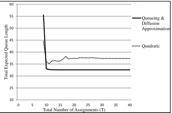
In the next subsection, we use a numerical example to illustrate the Backward Se-lection Heuristic Algorithm by applying queueing model and diffusion approximation model as congestion performance measures. We will also compare these two models with convex quadratic model at the end.
Note that we do not use this algorithm to solve Pq, since it is a mixed integer
Algorithm 2 Backward Selection Heuristic Algorithm t←M N;
for i= 1→N, k = 1→M do dn,k ←1;
end for
α← α∗(d) as defined in Problem P(d); for i= 1→N, k = 1→M do
if αn,k= 0 then
dn,k ←0;
end if end for t←PN
n=1
PM k=1dn,k
while t > T do
for i= 1 →N, k= 1→M do if dn,k = 0 then
Ψn,k ← ∞;
else
dn,k ←0;
Ψn,k ← Ψ(d) as defined in Problem P(d);
dn,k ←1;
end if end for
(i, k)←arg minn,kΨn,k;
dn,k ←0;
t←t−1; end while
2.7.2
Numerical Example I
We consider an example with five servers (M = 5) and eight types of services (N = 8). We assume that the overall arrival rate, the transition probability matrix of the DTMC determining the customer class, and the service time distributions are known. We can calculate the variance-covariance of arrival process needed for diffusion approximation model from the given arrival rate and transition probability matrix. The upper limit of the total number of assignments is T = 12.
transition probability matrix Θ =
.0333 .3000 .1905 .0952 .0476 .0994 .1068 .1271 .2667 .0667 .1905 .0952 .0476 .0994 .1068 .1271 .1569 .1765 .3000 .0167 .0167 .0994 .1068 .1271 .1569 .1765 .0333 .2833 .0167 .0994 .1068 .1271 .1569 .1765 .0667 .0333 .2333 .0994 .1068 .1271 .1569 .1765 .1905 .0952 .0476 .0333 .0667 .2333 .1569 .1765 .1905 .0952 .0476 .2000 .0333 .1000 .1569 .1765 .1905 .0952 .0476 .0667 .2000 .0667
.
The steady-state distribution is
π= [ .1569 .1765 .1905 .0952 .0476 .0994 .1068 .1271 ].
This example has a special design so that eight customer types are separated into three groups before generating transition probability matrix: a group of services with negatively correlated traffic streams among group members, and two groups of services with positively correlated traffic streams among group members. The traffic streams between any two types in different groups are independent. This design can be achieved by properly choosing the transition probability so that Θn,j = πj and
Θj,n =πn if we want the traffic stream of type n and j to be independent.
ob-tained by Eq. (2.5.2), Σ =
16.93 4.24 0 0 0 0 0 0
4.24 19.58 0 0 0 0 0 0
0 0 33.30 −5.56 −2.03 0 0 0
0 0 −5.56 19.43 −1.02 0 0 0
0 0 −2.03 −1.02 9.48 0 0 0
0 0 0 0 0 11.61 .91 .90
0 0 0 0 0 .91 12.31 1.20
0 0 0 0 0 .90 1.20 15.06
, R =
1 .23 0 0 0 0 0 0
.23 1 0 0 0 0 0 0
0 0 1 −.22 −.11 0 0 0
0 0 −.22 1 −.07 0 0 0
0 0 −.11 −.07 1 0 0 0
0 0 0 0 0 1 .08 .07
0 0 0 0 0 .08 1 .09
0 0 0 0 0 .07 .09 1
.
From the correlation coefficient matrix, we observe that the arrival processes of service 1 and 2 are positive correlated with each other and independent of the rest of the services. The arrival processes of service 3, 4, and 5 are negative correlated with each other and independent of all the rest of the services. The arrival processes of service 6, 7, and 8 behave similarly to those of 1 and 2 but with weaker correlations.
Queueing Model
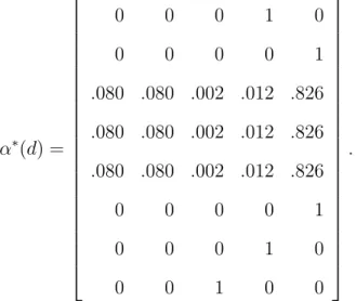
In the initial step of the algorithm, we assume all assignments are available on every server and solve for the optimal routing policy. Assumingdn,k = 1 for alln and
k, the following initial routing policy matrix is obtained by solvingP(d),
α∗(d) =
0 0 0 1 0
0 0 0 0 1
.080 .080 .002 .012 .826 .080 .080 .002 .012 .826 .080 .080 .002 .012 .826
0 0 0 0 1
0 0 0 1 0
0 0 1 0 0
.
As we expected, we observe that the traffic streams with positive correlations are routed into different servers, while the traffic streams with negative correlations are routed into common servers.
In the next step, we remove all assignments with α., .= 0. The total number of assignments left is 20. In terms of the total expected queue length, the system with these 20 assignments can perform as well as the system with 40 assignments, i.e., all assignments being enabled to provide every type of service. Since the desired total number of assignments isT = 12, we need to proceed with the algorithm further and remove eight more assignments.
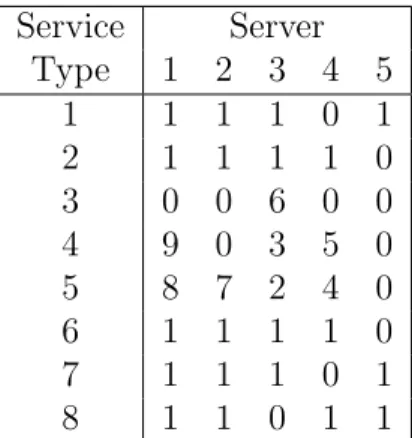
Service Server
Type 1 2 3 4 5
1 1 1 1 0 1
2 1 1 1 1 0
3 0 0 6 0 0
4 9 0 3 5 0
5 8 7 2 4 0
6 1 1 1 1 0
7 1 1 1 0 1
8 1 1 0 1 1
Table 2.1: Example I: Removal Progress of Heuristic Algorithm Using Queueing Model
We repeat the elimination process until the number of assignments left is less than or equal to 12. The zeros on the table mean those assignments remain on the servers after the completion of the heuristic algorithm. Based on this table, we determine the service assignment of the system. The assignment policy out of this heuristic algorithm d∗h should be to enable server k to provide service type n if and only if it is zero in the row n and column k in Table 2.1.
Along with the above assignment policy, we determine the routing policy out of the heuristic algorithm:
α∗∗h =
0 0 0 1 0
0 0 0 0 1
.139 .080 0 .023 .758 0 .119 0 0 .881
0 0 0 0 1
0 0 0 0 1
0 0 0 1 0
0 0 1 0 0
.
Diffusion Approximation Model
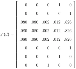
Assumingdn,k = 1 for all nand k again, another initial routing policy is obtained
by solving ˜P(d),
˜ α∗(d) =
0 0 0 1 0
0 0 0 0 1
.080 .080 .002 .012 .826 .080 .080 .002 .012 .826 .080 .080 .002 .012 .826
0 0 0 0 1
0 0 0 1 0
0 0 1 0 0
.
This initial routing policy comes out to be exactly the same as the initial routing policy obtained by queueing model. Similar to what we did for queueing model, we further proceed with the algorithm and use the Table 2.2 to show the removal progress.
Service Server
Type 1 2 3 4 5
1 1 1 1 0 1
2 1 1 1 1 0
3 0 0 6 0 0
4 9 0 3 5 0
5 8 7 2 4 0
6 1 1 1 1 0
7 1 1 1 0 1
8 1 1 0 1 1
Table 2.2: Example I: Removal Progress of Heuristic Algorithm Using Diffusion Ap-proximation Model