GENOTYPE-PHENOTYPE SIMILARITY
TESTING AND METHODS FOR INTEGRATING
MULTIPLE DATA SOURCES IN GENETIC
ASSOCIATION
Gregory M. Mayhew
A dissertation submitted to the faculty of the University of North Carolina at Chapel Hill in partial fulfillment of the requirements for the degree of Doctor of Public Health in the Department of Biostatistics.
Chapel Hill 2013
Approved by:
Dr. Fred A. Wright Dr. Fei Zou
c
2013
Abstract
GREGORY M. MAYHEW: Genotype-Phenotype Similarity Testing and Methods for Integrating Multiple Data Sources in Genetic Association
(Under the direction of Dr. Fred A. Wright and Dr. Fei Zou)
Genome-wide association studies (GWAS) have been successful in identifying SNP
associations for many complex traits. However, for any single trait, published and
validated SNPs typically explain only a small part of the genetic heritability estimated
to be explained by genetic variation. New methods are needed that can detect small
effect sizes and overcome challenges presented by true biological architecture, including
causal variants that are not directly genotyped, and allelic heterogeneity. Here we
propose a likelihood ratio test (LRT) approach in two forms to perform SNP-set analysis
in GWAS. The first form compares the similarity of traits between pairs of unrelated
individuals to that of genotypes. The second form jointly tests trait-genotype similarity
and regional maximal trait-SNP association. In simulation studies, these methods show
favorable power compared to popular alternative approaches.
The basic idea of trait-similarity approaches is that, for genomic regions harboring
loci that affect a trait, individuals with similar genotypes/haplotypes should have more
similar traits. Therefore, as a nonparametric alternative to likelihood-based testing,
we consider a statistic that directly correlates genetic and trait similarity. Due to the
comparison of dependent pairs of individuals, standard distributional approximations
for correlation coefficient testing do not apply. Monte Carlo approaches to evaluating
moment matching statistic for SNP-set analysis.
Finally, we discuss challenges in performing GWAS meta-analyses for differing
dis-eases, and for joint testing of association with multiple traits (pleiotropy). A key issue
is that the alternative hypothesis should be restricted to joint effects, and standard
testing procedures are not adequate. We propose practical schemes to (i) create
statis-tics that are sensitive only to the intended alternative, and (ii) cyclic shift genome-wide
Acknowledgments
I am deeply thankful and fortunate to have worked with Fred and Fei. Their talents
and knowledge continuously amaze me. I look forward to discovering, over time, all
that I have learned during this training. I am also extremely grateful to Fred for his
financial support.
Thank you to the professors and staff of the Biostatistics department.
Thank you to Mike, Kari, and Yun for serving on my committee. I greatly appreciate
their willingness to help in this process. I would also like to thank Mike for allowing
me to work with his team and use their data in my thesis.
Table of Contents
List of Tables . . . ix
List of Figures . . . xi
1 An Extended Similarity-Based SNP-Set Approach for GWAS . . . 1
1.1 Introduction . . . 1
1.2 Methods . . . 4
1.2.1 Testing . . . 4
1.2.2 Numerical Optimization . . . 6
1.2.3 Linkage Disequilibrium Blocks . . . 7
1.2.4 Simulation Studies . . . 9
1.3 Results . . . 11
1.3.1 Simulation Studies . . . 11
1.3.2 Application to CF Data . . . 13
1.4 Discussion . . . 14
1.5 Exploration of LD Block Algorithm Parameters . . . 17
1.6 Tables and Figures . . . 18
2.2.1 Siemiatycki Moments . . . 38
2.2.2 Approximation of the Permutation Distribution . . . 40
2.3 Results . . . 42
2.3.1 Application to CF Data . . . 42
2.3.2 Application to Winter Dysentery Study . . . 43
2.4 Discussion . . . 45
2.5 Tables and Figures . . . 45
3 Combined Data Analysis . . . 60
3.1 Introduction . . . 60
3.1.1 Problems with Traditional Parametric Approaches . . . 61
3.2 Methods . . . 64
3.2.1 Cyclic Shift . . . 64
3.2.2 Independent Studies . . . 65
3.2.3 Independent Studies (Irwin-Hall Approach) . . . 65
3.2.4 Non-independent Studies . . . 69
3.2.5 Non-independent Studies,p-values . . . 70
3.2.6 Simulations . . . 71
3.2.7 Real Data Analysis . . . 72
3.3 Results . . . 72
3.3.1 Simulation Studies . . . 72
3.3.2 Real Data Analysis . . . 73
3.4 Discussion . . . 74
3.5 Tables and Figures . . . 75
List of Tables
1.1 Empirical Type I Error Rates for Continuous Trait Type I error rates for each LD block size (10,30,50 SNPs) are shown for significance levels α = 0.05,0.005,and 0.0005. The LD blocks were randomly selected from chromosomes 12 through 22. Each error rate is based on 120,000 simula-tions using HapMap 3 CEU genotypes and sample size of n = 1000. To calculate p-values for LRT1 and LRT2, we used ˆπ1 = 0.599 and
ˆ
π2 = 0.932, which were obtained using all 360,000 simulations. . . 31
1.2 Empirical Type I Error Rates for Binary Trait Type I error rates for each LD block size (10,30,50 SNPs) are shown for significance levels α = 0.05,0.005,and 0.0005. The LD blocks were randomly selected from chromosomes 12 through 22. Each error rate is based on 120,000 simula-tions using HapMap 3 CEU genotypes and sample size of n = 1000. To calculate p-values for LRT1 and LRT2, we used ˆπ1 = 0.564 and
ˆ
π2 = 0.932, which were obtained using all 360,000 simulations. . . 32
1.3 TopLRT1 Results from the Genome-scan of the CF Data using LD Block
Regions as Testing Units, Along with the Most Significant SNP in Each Region as Reported by Wright et al.36 . . . 33
1.4 TopLRT2 Results from the Genome-scan of the CF Data using LD Block
Regions as Testing Units, Along with the Most Significant SNP in Each Region as Reported by Wright et al.36 . . . 34
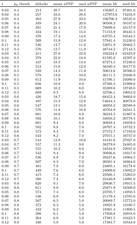
1.5 For several combinations of the LD block algorithm parameters tand pk
threshold, we characterize the block definitions using the total number of blocks of size 3 or more, mean and median SNPs within each block, and mean and median block size. Analysis used all chromosome 22 SNPs for the CF data. . . 35
2.4 Siemiatycki Moments: Coefficients for Computing E(Z3) . . . 57
2.5 Siemiatycki: Coefficients for Computing E(Z4) . . . . 58
2.6 Top Sassoc1 Results from the Genome-scan of the CF Data using LD Block Regions as Testing Units, Along with the Most Significant SNP in Each Region as Reported by Wright et al.36 . . . 59
3.1 Simulation study: H00, independent, Irwin-Hall . . . 89
3.2 Simulation study: H00, independent, cyclic shift . . . 90
3.3 Simulation study: H00, non-independent, trait correlation 0.25, cyclic shift 91 3.4 Simulation study: H00, non-independent, trait correlation 0.50, cyclic shift 92 3.5 Simulation study: H00, non-independent, trait correlation 0.75, cyclic shift 93 3.6 Simulation study: H00, non-independent, p-values only observed, trait correlation 0.50, cyclic shift . . . 94
3.7 Simulation study: HA, independent, Irwin-Hall . . . 95
3.8 Simulation study: HA, independent, cyclic shift . . . 96
3.9 Simulation study: HA, non-independent, trait correlation 0.25, cyclic shift 97 3.10 Simulation study: HA, non-independent, trait correlation 0.50, cyclic shift 98 3.11 Simulation study: HA, non-independent, trait correlation 0.75, cyclic shift 99 3.12 Simulation study: HA, non-independent, p-values only observed, trait correlation 0.50, cyclic shift . . . 100
3.13 Top results from all seven WTCCC studies . . . 101
3.14 Top results from CAD+HT+T2D . . . 102
3.15 Top results from CD+RA+T1D . . . 103
List of Figures
1.1 Power Study for Continuous Trait Power at each combination of block size (10,30,50 SNPs), heritability (0.05,0.10,0.15,0.20), and number of causal SNPs (1,2,3,4,5) is based on 3000 simulations using HapMap 3 CEU genotypes and sample size of n = 1000. To calculate p-values for LRT1 and LRT2, we used ˆπ1and ˆπ2 values from the null simulations.
The significance threshold was set at 0.05/25,000 to reflect use of the proposed methods in a genome scan. Causal SNPs were removed from the datasets before analysis. . . 19
1.2 Power Study for Binary Trait Power at each combination of block size (10,30,50 SNPs), heritability (0.05,0.10,0.15,0.20), and number of causal SNPs (1,2,3,4,5) is based on 3000 simulations using HapMap 3 CEU genotypes and sample size of n = 1000. To calculate p-values for LRT1
and LRT2, we used ˆπ1and ˆπ2 values from the null simulations. The
sig-nificance threshold was set at 0.05/25,000 to reflect use of the proposed methods in a genome scan. Causal SNPs were removed from the datasets before analysis. . . 20
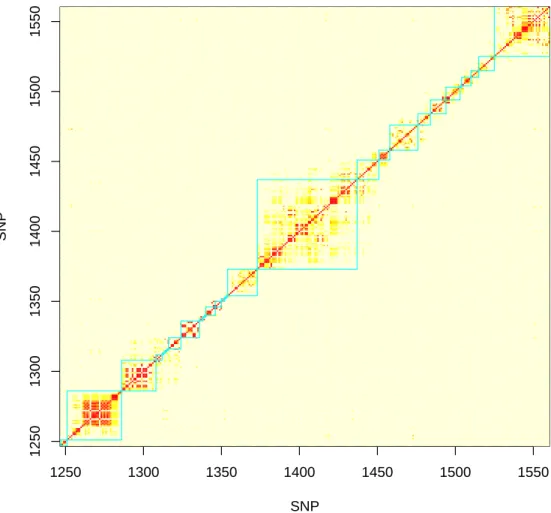
1.3 The LD Block Algorithm Applied to Several Hundred SNPs on Chro-mosome 22 for the CF Data The SNP sets formed by the algorithm are outlined in green. Red and yellow shades depict varying pairwise SNP r2. 21
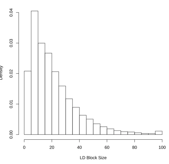
1.4 Distribution of LD Blocks with 3 or more SNPs for the CF Data On the autosomes, our LD block algorithm identified 25,066 blocks containing three or more SNPs. Mean and median block sizes were 21.6 and 17.0, respectively. . . 22
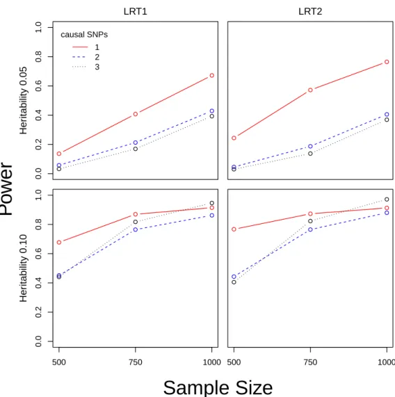
1.5 Power Versus Sample Size The figure depicts the relationship between power and sample size for LRT1 and LRT2, using continuous traits and
1.6 QQ-plots for Binary Trait Null Simulations To account for possible lack of fit and to better investigate p-value tail behavior, we ran a larger number of simulations for binary traits. The 360,000 simulations had two potentially extreme observations. . . 24
1.7 GCTA Heritability Rank versus LRT1 Statistic Rank The figure depicts
the relationship between GCTA39 heritability estimates and the LRT1
statistic when entire chromosomes are treated as testing units. For each chromosome, circle area is proportional to the number of genotyped SNPs. 25
1.8 The LRT1 statistic is highly correlated with the score-like sum y0Xy,
whether the phenotype y is continuous or binary. Using genotypes from a single block of size 30, we show LRT1 versus the score-like sum on the
rank scale for 1000 null simulations of y. . . 26
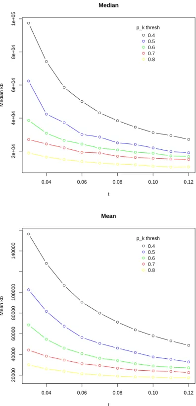
1.9 We show the relationship between median (and mean) block size and LD block algorithm parameter values. Analysis used all chromosome 22 SNPs for the CF data. . . 27
1.10 We show the relationship between the proportion of SNPs assigned to a block and LD block algorithm parameter values. Analysis used all chromosome 22 SNPs for the CF data. . . 28
1.11 We applied the LD block algorithm to all chromosome 22 SNPs for the CF data using three parameter settings. The block definitions formed by the algorithm for several hundred SNPs are outlined in green. Red and yellow shades depict varying pairwise SNP r2. . . . 29
1.12 We applied the LD block algorithm to all chromosome 22 SNPs for the CF data twice, once from beginning to end (forwards), and once back-wards, both usingt = 0.05 andpk threshold of 0.5. The block definitions
formed by the algorithm for several hundred SNPs are outlined in green. Red and yellow shades depict varying pairwise SNP r2. . . . 30
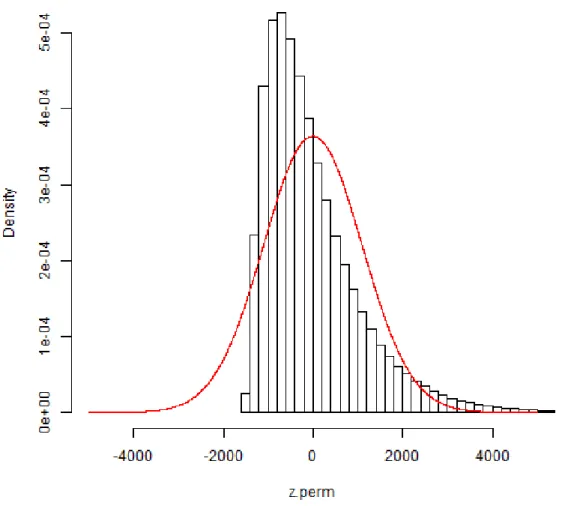
2.1 Histogram of 106 sample permutations of a Mantel statistic, with the
normal density approximation using the first two exact moments. The Mantel statistic correlated phenotypic similarity and genotypic similarity over a 21-SNP region from the CF study.36 . . . . 46
2.3 For three regions on chromosome 11, we show observed versus expected qq-plots for 106permutations of the Mantel statistic for the three moment
(Gamma) and four moment (Pearson) approximations. . . 48
2.4 The top panel shows −log10 p-values for Sassoc1 for the CF data. Each
p-value is computed for a moving window of +/− 10 SNPs around the center SNP. The qq-plot for a single 21-SNP window shows that the ap-proximating p-values are approximately uniform under 106 permutations. 49
2.5 We show −log10 p-values for Sassoc1 from the genome-scan of the CF
data using LD block regions as testing units versus results using LRT1
(Chapter 1). . . 50
2.6 Performance of the proposed approach for space-time clustering anal-ysis of the cattle data. The right column panels show a histogram of
SM antel, along with the normal density (gray) and our proposed (black)
approximations, as well as a qq-plot of observed approximatingp-values versus expected for 106 permutations. The left column panels show
re-sults for SKnox for 106 permutations, along with density fits based on
the Poisson (dashes) and Barton-David (dots) approximations, as well as our proposed density fit (solid). The lower left panel shows the true permutation p-values for all possible outcomes, compared to that of the approximation. . . 51
2.7 Manhattan plot of Sassoc1 results from the genome-scan of the CF data
using LD block regions as testing units . . . 52
2.8 QQ-plot of Sassoc1 results from the genome-scan of the CF data using
LD block regions as testing units . . . 53
3.1 Histograms of the maximum log-likelihood ratio for simulation setting (i) where neither study shows association and (ii) where a single study shows association. . . 76
3.2 Contour plot of the maximum log-likelihood using a single simulated dataset for setting (i) where neither study shows association. Along the axes, we show maximum log L(β1,0) and maximum log L(0, β2). The
3.3 Contour plot of the maximum log-likelihood using a single simulated dataset for setting (ii) where a single study shows association. Along the axes, we show maximum log L(β1,0) and maximum log L(0, β2).
The two points in each figure correspond to the maximum likelihood estimate ( ˆβ1, ˆβ2) using the unrestricted likelihoodL(β1, β2). . . 78
3.4 Kernel density plots of the maximum log-likelihood ratio for simulation setting (i) where neither study shows association (heritability for β1 and
β2 both zero) and (ii) where a single study shows association (0.05
heri-tability forβ1, and 0 forβ2), as well as a third setting (0.025 heritability
for β1, and 0 for β2). . . 79
3.5 The exact distribution of the sum of independent within-study ranks for N = 2. The Irwin-Hall density is overlayed. . . 80
3.6 Exact p-values versus Irwin-Hall approximation p-values (−log10 scale)
for a null study using N = 2 andM = 100. . . 81
3.7 Qq-plot of Irwin-Hall approximationp-values for a null study usingN = 2 and M = 100. . . 82
3.8 The rejection region (rank scale) for the Irwin-Hall approach for N = 2 and M = 100. Light gray indicates the region for p ≤ 0.05, and dark gray indicates the region for p ≤ 0.05/M. As an illustration, we show ranks from a single null dataset. . . 83
3.9 The rejection regions (t-statistic scale) for the Irwin-Hall approach and Fisher’s method for N = 2 and M = 100. As an illustration, we show t-statistics from a single null dataset. . . 84
3.10 The lookuptable shows relationships between correlation of bivariate nor-mal random variables, their rank correlation, and rank correlation of their p-values. To make the table, we generated 107 pairs of bivariate
normal variables for for each small increment across 0 to 1. . . 85
3.11 For a simulation study, we show autocorrelation plots for observed sum-mary statistics and sumsum-mary statistics under two cyclic shifts. We also show pairwise SNPr2 in the region. The autocorrelation plots show that
3.12 For a region containing 200 SNPs, we show r2 between within-study ranks for every pair of SNPs, separately for observed ranks and for ranks under cyclic shift. . . 87
Chapter 1
An Extended Similarity-Based
SNP-Set Approach for GWAS
1.1
Introduction
Genome-wide association studies (GWAS) aim to identify single-nucleotide
poly-morphisms (SNPs) associated with complex traits. Routine, first-pass approaches to
GWAS data analysis involve association testing for individual SNPs, and the resulting
p-values are compared to genome-wide significance thresholds to control overall type I
error. Attaining significance for any individual SNP test may be difficult due to
sev-eral factors, including stringent genome-wide testing thresholds and modest effect sizes.
Additional challenges are also presented by the true biological architecture, including
the fact that causal variants may not be genotyped, or that multiple causal variants
may be present in a single region, thus diluting the signal. For both of these situations,
we may gain power by considering entire sets of SNPs simultaneously, as an adjunct
to individual SNP testing. When a single SNP is causal but not genotyped, it may be
in linkage disequilibrium (LD) with multiple SNPs in a set, such that analysis of the
works to aggregate the signal from multiple SNPs with small effects, and can
poten-tially capture signal from interactions, even if not explicitly modeled.37 In this paper
we focus entirely on regional SNP set testing, rather than set-based testing involving
multiple genes in a pathway.15
Several methods for regional SNP-set analysis have been proposed.37,19,33 These
ap-proaches depend importantly on the assignment of SNPs to sets. Methods applied
in practice include use of fixed-width sliding windows1 and assignment of SNPs to
genes and pathways.16 Wu et al.37suggested that grouping strategies based on
biologi-cally meaningful genomic features may result in additional power gains. Such grouping
strategies include assigning SNPs to genes, pathways, evolutionarily conserved regions,
or haplotype/linkage disequilibrium (LD) blocks. In principle, SNP-set analysis
ap-proaches can also gain power by reducing the number of tests performed in a genome
scan. Analysis of SNP sets that are not highly correlated also offers potentially higher
power, as Bonferroni false discovery control is less conservative than for individual SNPs
that are highly correlated.
Tzeng et al.31 divided SNP-set methods (as distinct from the assignment of SNPs
to sets) into four categories. The first category includes methods that use a weighted
sum of genotypes across markers in the SNP set. Methods in the second category
model the genetic similarity of pairs of individuals, and are informed by the theoretical
framework of U-statistics.34 The third category includes methods that treat
individ-ual genetic effects as random, with testing for variance-components (VC). The fourth
category collects the remaining methods. As noted by Tzeng et al.,31 VC methods
in the third category have been shown to perform favorably when evaluating genetic
quan-measurements on haplotype similarities. Thus, their approach belongs to the second
category. However, they have shown that their approach can also be viewed as in
category three, as parameters in their similarity regression are equivalent to VCs in a
haplotype random-effects model.30Thus, SIMreg is an essential standard of comparison
for regional simultaneous testing of multiple main genetic effects. The SKAT method
of Wu et al.38 is a similar category three approach. Although SKAT has primarily
been proposed in the context of analysis of rare variant sequencing data, it is
popu-lar, and the statistic is motivated by connections to VC modeling. Thus, performance
comparisons may be additionally informative.
Regional SNP-set testing may be viewed as occupying a “middle” genomic scale,
in which software such as GCTA39 typifies the large-scale extreme of using the entire
genome, and individual SNP testing represents the smallest scale. From this point
of view, and considering the testing benefits of dividing the genome into nearly
in-dependent units, we advocate regional SNP-set testing by LD blocks (although our
proposed approach is applicable to any SNP set). We present a fast method to identify
LD blocks, forming non-overlapping SNP sets as the testing units. We also note that
when applying similarity-regression or other regional SNP-set testing approaches, an
outstanding question remains regarding the role of individual SNPs. If both a SNP and
surrounding region are individually significant, it may be unclear how to apportion the
evidence, and whether evidence from the SNP-set is dominated by the most significant
SNP, or represents true additional evidence.
Here we propose a likelihood ratio test (LRT) approach to perform SNP-set analysis
in GWAS. The LRT appears in two forms (i) a version, comparable to SIMreg, which
compares similarity of traits to that of genotypes. Although the formal model is for
(ii) performs joint testing of genotype similarity and of regional maximal
trait-SNP association, in a single likelihood ratio test. Here a key problem is to provide
appropriate p-values for the joint test, accounting for multiple testing of the
trait-SNP associations across the region. In simulations, we demonstrate the validity of the
proposed tests and investigate power under a range of alternative settings, including
varying trait heritability, number of casual SNPs, and SNP set size. The utility is
further illustrated by a re-analysis of the cystic fibrosis (CF) [MIM 219700] genome
modifier study of Wright et al.36
1.2
Methods
1.2.1
Testing
Let Yi denote the continuous trait for individual i, i = 1, ..., n. We assume that
the genotypes have been numerically coded to the number of minor alleles, and further
scaled and normalized so that each SNP has mean 0, variance 1. LetXij be the Pearson
correlation coefficient between the genotypes of individuals i and j, using all M SNPs
in the current SNP set. We will handle covariates by assuming that the trait values and
genotypes have already been separately residualized for the covariates using a multiple
linear regression model. Inclusion of covariates technically affects the degrees of freedom
available for parameter estimation, but here we assume thatn is large compared to the
number of fitted covariates.
We model then×1 vectorY as an observation from a multivariate normal density,
Letl1 denote the log-likelihood for the model evaluated at the maximum likelihood
estimate (MLE) for which ρ is constrained to be non-negative, and let l0 denote the
log-likelihood at the MLE for the nested model with ρ = 0. The likelihood ratio
test (LRT) statistic is 2(l1 −l0), denoted by LRT1. Under the null hypothesis, the
asymptotic distribution ofLRT1is mixture of a point mass at 0 and a chi-square density
with 1 degree of freedom,26 i.e. the cumulative distribution function is F(LRT 1) =
π1Fχ2
0(LRT1) + (1−π1)Fχ21(LRT1), with the term π1 appearing due to the directional
alternative constraint. In contrast to a standard constrained setting, which applies
to linear mixed models where the data vector can be partitioned into a large number
of independent and identically distributed subvectors, π1 can depart markedly from
1 2.
7 Here we estimate π
1 directly as the proportion of SNP sets with ˆρ = 0. This
approach is unbiased if no gene set is associated with the trait, and slightly conservative
otherwise. Our LRT1 model is similar to that of SIMreg,31 which uses a
haplotype-based similarity matrix and an approximate score statistic for testing. In contrast, we
employ a correlation-based genotype similarity matrix and a true maximum likelihood
ratio.
Recognizing that individual SNPs may play a dominant role, potentially obscuring
additional genotype-phenotype similarity signal, we also propose an expanded model
including a main effect for a single SNP in the SNP set. For the chosen SNP, the
genotype for the ith individual is denoted by z
i, and our model assumes E(Yi) =
µ+βzi, with variance-covariance matrix as described above. For this model, we are
interested in H0 : {β = 0, ρ = 0}, vs. HA : {β 6= 0 or ρ > 0}. We use l2 to
denote the log-likelihood at the MLE, constrained according to HA, and l0 to denote
the log-likelihood at the MLE constrained by H0, and define LRT2 = 2(l2−l0). Under
the null hypothesis, the asymptotic distribution of LRT2 is a chi-square mixture with
distribution functionF(LRT2) = π2Fχ2
use empirical estimation ofπ2 as the proportion of SNP sets with ˆρ= 0.
The approximating null distribution for LRT2 applies only if the SNP is chosen
at random. However, for computational efficiency, for each SNP set we use the SNP
exhibiting the greatest evidence of trait association in individual SNP testing, and our
null distribution for LRT2 must account for this selection. A within-set Bonferroni
approach is applicable, but unnecessarily conservative. Instead, we use the method of
Moskvina and Schmidt21 to adjust for the implicit multiple testing in employingLRT2
on the “best” SNP within each set. This method computes an effective number of tests
(Keff) for a set of correlated SNPs within the SNP set. Accordingly, if p represents the
p-value forLRT2 within a SNP set (i.e., LD block), we compute a set-based adjustment
pset=Keff×p. As described below, we construct non-overlapping SNP sets from linkage
disequilibrium (LD) blocks, which show dramatically lower serial correlation than do
individual SNPs.
For binary Y (e.g., 1=case, 0=control), we use the same likelihood approach,
al-though the data are not normal. Nonetheless, as we show below, the type I error
properties remain favorable (though slightly conservative) under this approximation.
We note that the π values are estimated from the data, thus reflecting empirical
prop-erties of the observed data.
1.2.2
Numerical Optimization
We perform numerical optimization of the likelihoods using the optim() function in
l(µ, β, σ2, ρ) = −n
2log(2π)− 1
2log|V| − 1
2(y−µ−βz)
TV−1(y−µ−βz), (1.2)
whereV =σ2[I(1−ρ) +ρX].
Maximization of the likelihood is simplified using matrix identities described below.
First, we use G00 to denote the original M ×n matrix of SNP genotypes (or genotype
residuals if adjusting for covariates). G0 is the resulting matrix when each row has been
centered and scaled to have mean 0 and variance 1. Let G be the resulting matrix
when each column of G0 has been centered and scaled to have mean 0 and variance
1/(M−1). Finally, we haveGTG=X. In genome-wide association studies, the number
of individuals n is typically much larger than the M SNPs in a set. We have
[I(1−ρ) +ρGTG]−1 = 1 1−ρI−
ρ (1−ρ)2G
T
(I+ ρ
1−ρGG
T
)−1G (1.3)
and
|I(1−ρ) +ρGTG|= (1−ρ)n|I+ ρ 1−ρGG
T|, (1.4)
which employ the Woodbury matrix identity (equation 1.3) and the Sylvester
deter-minant theorem (equation 1.4). These identities considerably reduce computation, by
working with theM ×M matrix GGT rather than directly with the n×n matrix V.
1.2.3
Linkage Disequilibrium Blocks
We have developed a fast algorithm to identify non-overlapping genomic intervals
of high linkage disequilibrium for use as SNP sets. We here refer to these intervals
high r2 than deducing the underlying haplotype structure. Thus the size of the blocks
we use tends to be greater than that identified using approaches as described in The
International HapMap Consortium.29 The algorithm moves sequentially across each
chromosome, identifying successive blocks, with a practical minimum block size of 3
SNPs. LetK denote an integer, chosen to be large enough to exceed the likely number of
SNPs in the largest LD block. For the genotyping platform used in the CF study,K =
100 appeared to suffice, but might be larger for a platform with higher SNP density.
A block is identified by first starting from an initial SNP m and creating a putative
block consisting of SNPs {m, m+ 1, ...m+K}. Subsetted blocks{m, m+ 1, ..., m+k}
are then considered for k = K, K −1, ...,, continuing until an “optimum” block is
identified according to the following criterion. For each subsetted block, let Rk denote
the corresponding k×k matrix of SNP r2 values. Define p
k as the proportion of the
elements of Rk exceeding a pre-specified threshold t, where t = 0.05 in our examples.
Also define ∆k = pk −pk−1, where ∆1 ≡ 1. Finally, we obtain the optimum block
as the set {m, m+ 1, ...m+k0}, where k0 = maxk{k : I(∆k <= 0)I(pk > 0.5)}. The
choice of pk >0.5 appeared to suffice for the platform used in the CF study, and is at
the discretion of the user. Other thresholds may perform better for studies with other
genotyping platforms.
For each chromosome, we start withm= 1, and after obtaining the solutionk =k0,
begin the next block at positionk0+ 1, etc. The algorithm lacks symmetry, in the sense
that slightly different LD blocks may be identified if the investigator reverses the order
of the SNPs per chromosomes. However, the algorithm is fast and can easily be run on
1.2.4
Simulation Studies
To investigate the performance of our proposed methods, we performed simulations
using HapMap 3 CEU genotype data. To match the simulations to data analysis of the
real CF data, as well as to perform SNP subset analysis without the complications of
shifting block definitions, we first applied our LD block algorithm to the CF data (1978
individuals, 556,446 autosomal SNPs). In this manner we divided the genome into
non-overlapping LD blocks, each containing three or more SNPs (25,066 blocks), and applied
the same LD block boundaries throughout our analyses. Starting with chromosome 22
and moving backward through the genome, we identified blocks containing exactly 10,
30, and 50 SNPs, until a sufficient number were identified (stopping at chromosome 12),
and randomly sampled 10 of each size to obtain 30 LD blocks. For each of the 30 blocks,
we generated 300 sets of genotypes for n = 1000 individuals, by randomly sampling
haplotype pairs from the 234 phased CEU haploid genomes available in HapMap 3
(1,387,466 autosomal SNPs available genome-wide).
Continuous Traits
To study type I error, we randomly sampled n = 1000 quantitative traits from the
N(0,1) distribution, 40 times for each of the 9000 sets of genotypes, to generate 360,000
simulations. To investigate statistical power, we simulated quantitative traits under a
range of underlying causal SNP counts (s = 1,2,3,4,5) in an LD block, as well as
under several trait heritability settings (h2 = 0.05,0.10,0.15,0.20). First, for each of
the 30 LD blocks, five SNPs were identified as underlying causal SNPs as follows : (i)
one set of genotypes was randomly selected from the 300 in the study; (ii) to select the
s causal SNPs, the first SNP was chosen at random, the second SNP (if s > 1) was
chosen to have the smallest r2 with the first, the third SNP (if s > 2) was chosen to
sets of genotypes, we generatedn = 1000 quantitative traits for each of the 20 possible
combinations of (s = 1,2,3,4,5) and (h2 = 0.05,0.10,0.15,0.20), to obtain 180,000
simulations. For each, we scaled the s vectors of causal SNP genotypes to have mean
0 and variance 1, and summed the resulting values to obtain the causal genetic effect
for the ith individual, which we denote by c
i. We setσc2 equal to the sample variance
(σ2
c =
1
n−1
Pn
i=1(ci −c)¯2) and for the specified heritability h2 = σ 2
c
σ2
c+σ2e, solved for σ
2
e.
Finally, we generated each traitYi as a random sample from theN(ci, σ2e) distribution.
Simulations were analyzed using our proposed methods LRT1 and LRT2, as well
as three existing methods, (i) the SIMreg program (using weight matrix inverse allele
frequencies on the diagonal and zeros otherwise), (ii) the SKAT program (using the
unweighted linear kernel - use of the default weighted linear kernel performed uniformly
more poorly and is not shown) and (iii) using the minimum SNPp-value as a statistic,
employing the Moskvina and Schmidt21 correction for multiple testing within the SNP
set. Prior to analysis of each dataset, causal SNPs were removed and the remaining
SNPs considered to have been “genotyped.”
Binary Traits
To study type I error for binary traits, we used the same sets of genotypes described
above. A single vector of binary traits consisting of 500 zeroes and 500 ones was
randomly permuted, 40 times for each of the 9000 simulated sets of genotypes described
above, to obtain 360,000 null simulations.
To investigate statistical power, we used the same sets of genotypes and underlying
causal SNP counts as described above for continuous traits, to generate 180,000
alter-native genotype simulations. However, a modification was necessary for binary trait
sce-identical to the standardh2. For binary traits, in contrast to methods based on
thresh-olding of an underlying liability function, the definition here ensures comparability to a
continuous trait with the same heritability, as power is driven largely by the expected
genotype-conditional variability compared to total variability. To operationalize our
approach, we assumed an underlying logistic model, i.e. P(Yi = 1|ci) = θi = e
β0+β1ci
1+eβ0+β1ci. For a fixed {β0, β1}, the required expectation is easily computed over the n samples,
because var(Yi|ci) = θi(1−θi). Finally, we numerically solved for {β0, β1} using two
constraints: (i) the target h2, and (ii) the desired 1:1 case:control ratio, which implies
E(Y) = 12.
As for continuous traits, simulations were analyzed using LRT1, LRT2, SIMreg
(using thetrait=binomialGLM approach and weight matrix inverse allele frequencies on
the diagonal and zeros otherwise), SKAT (for dichotomous traits with unweighted linear
kernel and small sample p-value adjustment), and the Moskvina-Schmidt minimum
p-value approach. The individual SNP p-values used the normal approximation to the
Cochran-Armitage trend test for the 3×2 genotype-trait table. Causal SNPs were
removed from the datasets before analysis.
1.3
Results
1.3.1
Simulation Studies
Continuous Traits
Across the 360,000 null simulations, we obtained ˆπ1 = 0.599 and ˆπ2 = 0.932.
Em-pirical type I error rates were calculated as the proportion of simulations withp-values
smaller than the intended thresholds α= 0.05,0.005,0.0005. The results are shown in
be slightly conservative.
Power was evaluated separately for the various block sizes (Figure 1.1). As described
earlier, for each setting of block size, number of causal SNPs (s = 1,2,3,4,5), and
trait heritability (h2 = 0.05,0.10,0.15,0.20), 3000 simulations were performed. As
approximately 25,000 LD blocks are typically identified on the genome, the significance
threshold for eachpset was set at 0.05/25,000, to reflect use of the proposed methods in
a genome scan. We used the ˆπ1 and ˆπ2 values from the null simulations, as even under
the alternative hypothesis, these values are estimated with reasonable accuracy in a
genome scan. Figure 1.1 illustrates the dependence of power on h2 for a given block
size and s. LRT2 displayed power that was equal or better than any other method in
all settings. LRT1 also performed reasonably well, except for blocks of size 10. We
attribute the superior performance of LRT2 to the likely outcome that, for large s, at
least one of the SNPs will be in high linkage disequilibrium with at least one genotyped
SNP, providing a boost in performance overLRT1. The improvements in power for our
LRT methods over SIMreg, SKAT, and the minimum p-value is greatest in blocks of
size 50, when multiple causal SNPs are present.
To illustrate the effect of sample size on power for LRT1 and LRT2, we performed
additional simulations usingn = 500 and 750 individuals and plotted power estimates
along with results for n= 1000 (Figure 1.5). For trait heritability of 0.05, power gains
appeared approximately linear over the range ofnwe investigated. For trait heritability
of 0.10, power gains were greatest moving fromn= 500 to 750, and with reduced gain
when moving to n= 1000.
Binary Traits
good control of false positives and being slightly conservative.
Figure 1.2 shows the power results for binary traits, which are qualitatively similar
to the results for continuous traits. Again, LRT2 has approximately equal or better
power than any other method in any of the settings.
1.3.2
Application to CF Data
We applied our proposed methods ton= 1978 unrelated individuals used in the CF
genome modifier study of Wright et al.36 All of the subjects were homozygous for the
∆F508 genotype at CF T R[MIM 602421]. The continuous trait was the lung function
phenotype, adjusted for age and CF cohort, described in Taylor et al.28Residualization
adjustment was performed for sex and for genotype PCs as described in the original
study. On the autosomes, our LD block algorithm identified 25,066 blocks containing
three or more SNPs. An example of LD block partitioning and a histogram of LD
block sizes are given in Figures 1.3 and 1.4, respectively. For these data, ˆπ1 = 0.596
and ˆπ2 = 0.917, which are very close to the results from HapMap 3 simulations. We
report the results for LRT1 in Table 1.3 and those for LRT2 in Table 1.4, which show
the ten most significant LD block regions for each LRT statistic. In addition, the tables
show results for the most significant SNP in each region as reported by Wright et al.36,
and forLRT2 we report both ˆρand the remainingr2 attributable to the top SNP in the
block. As described further in Discussion, ˆρ may be interpreted as a heritability-like
quantity, computed on the genotype correlation matrix.
Both LRT statistics identified regions harboring top SNPs that had been previously
reported, including two LD block regions near AP IP [MIM 612491] on chromosome
11. The top region for both LRT statistics contained rs10836312, and both improved
In addition, the third most significant region identified by LRT1 (FDR q-value 0.138)
was near the P DCL [MIM 604421] gene on chromosome 9. In contrast, the most
significant original finding in the region by single-SNP analysis had an FDR q-value
of 0.886. The P DCL example is illustrative that, although LRT2 was shown to be
generally more powerful than LRT1, a region with no significant SNP can produce
higher relative evidence fromLRT1, because of the higher multiple comparisons penalty
on LRT2 and model parsimony of LRT1. For that region, LRT1 and LRT2 produce
similar ˆρ values near 0.07, but the top SNP has r2 = 0.0039. This ˆρ, interpreted as a
local heritability, seems very high. However, it is important to note that
correlation-based similarity matrices of unrelated individuals provide limited information relative
to traditional twin-based designs, and is likely subject to large winner’s curse effects.
To perform a genome scan, we recommend applying the LD block algorithm and
our proposed test statistics separately to each chromosome. The LD block algorithm
runs very fast. Each chromosome required between one and five minutes using a Linux
cluster (varying CPU speeds from 2.3 to 3.6 Ghz having between 4 and 8 GB memory),
when we analyzed the GWAS of Wright et al.,36 and LRT1 and LRT2 each required
per chromosome run times between 3 and 18 hours.
1.4
Discussion
The use of genotype-trait similarity for genetic mapping has a history dating at
least to Haseman-Elston linkage analysis.13 It is widely believed that similar methods
adapted for association mapping, such as SIMreg, can potentially capture signal from
multiple causal variants, for which analysis of individual SNPs would have little power.
this situation can be quite substantial. Analysis using trait similarity is in practice
typically preceded by analysis of individual SNPs, and seldom performed genome-wide
using overlapping windows as prescribed in Tzeng et al.31 The contribution of our
LRT2 is that it exploits the combined information from an individual SNP and from
the remaining correlated SNPs. It also provides a unifying framework and a single
p-value for the region, rather than a sequential approach of single-SNP mapping followed
by a regional test. As LRT2 appears to be superior to or at least equal in power to
other approaches, we argue that it may be run routinely as part of a standard genome
scan.
We argue that LD blocks constitute reasonable units of analysis, capturing the
correlation structures that form the basis of trait-genotype similarity approaches. This
choice also produces tests for which the serial correlation is low. OurLRT approaches
can of course be applied to other choices of gene sets, including the assignment of SNPs
to genes, or perhaps using external information, such as eQTL relationships.22 It may
also be of interest to examine much larger gene sets, such as entire chromosomes. At
that scale, software such as GCTA39is often used, to estimate narrow sense heritability
from the IBD relationships among the “unrelated” individuals. Although GCTA uses
a different model and different approach to quantifying genotype similarity, the spirit
of LRT is similar. Thus it may not be surprising that the heritability estimates for
GCTA and LRT, performed at the chromosome level for the CF data, are correlated
(rank correlation 0.83, see Figure 1.7).
Our multivariate normal model (written here for LRT2) can be expressed as the
linear mixed model Y = µ+βz +b+e, where b ∼ N(0, σa2X) is a vector of random
genetic effects,e ∼N(0, σ2
eI) is a vector of random errors, andb andeare independent.
V ar(Y) = σ2aX+σe2I = (σ2a+σ2e)[ σ
2
a
σ2
a+σe2
X+ σ
2
e
σ2
a+σ2e
I] (1.5)
Comparison with our multivariate normal model formulation varianceV showsρ=
σ2
a
σ2
a+σ2e and σ
2 =σ2
a+σe2. This formulation illustrates that the parameterρin our model
can be viewed as the “local” genetic heritability explained by the block, after correcting
for the most significant SNP in the block.
Our simulations appeared to indicate that SIMreg may have a power advantage over
LRT1, but not LRT2, for small block sizes, but bothLRT methods are more powerful
for larger blocks. The primary differences between SIMreg and theLRT approaches are
in the definition of similarity matrices and in our use of maximum likelihood ratios. The
slightly poorer performance of SKAT may be somewhat surprising, given its motivation
from VC models and general similarity in spirit to SIMreg. In addition, the
variance-covariance term in our LRT approaches (e.g. the quadratic form(y−µ)TV−1(y−µ)
in LRT1) are very similar to sums of squared score statistics across the SNPs in the
set (see, e.g. derivations in Zhou et al.,40) which is another way of expressing the
SKAT statistic. However, a key difference may lie in the use of double-centering in
our genotype matrices, first by SNP (which is essentially used for all of the methods)
and then again by individual. The second centering step was initially motivated by
computational considerations, in order to use the matrix identities described in
Meth-ods. However, it is worth exploring whether other choices of similarity matrices may
extract additional power from the data, and further elucidation may yield additional
improvements. Nonetheless, forLRT2 the primary advantage appears to lie in the joint
modeling of the top regional SNP and the additional background information in the
1.5
Exploration of LD Block Algorithm Parameters
As mentioned before, our procedure for identifying LD blocks was motivated by
testing considerations and high r2, rather than deducing the underlying haplotype
structure. Our choices of t = 0.05 and pk threshold of 0.5 appeared to suffice for
analysis of the CF data. However, it may be useful to examine the results of varying
the parameter values, and in particular try to find values that lead to average block
size near 10kb, for example.
Using all 8511 chromosome 22 SNPs from the CF study, we ran the algorithm
several times. Figure 1.9 shows mean and median block size for several combinations
of algorithm parameters. In addition, Figure 1.10 shows the proportion of all SNPs
that were assigned to a block. Note that blocks are defined as containing 3 or more
SNPs. Table 1.5 shows additional information, including total number of blocks, as
well as mean and median SNP count. The results suggest that increasing t and the
pk threshold towards higher values yields median block size closest to the 10kb target,
however we can also see that the proportion of SNPs assigned to a block decreases as
either parameter increases.
In Figure 1.11 we show block definitions for several hundred SNPs on Chromosome
22 for the CF Data, using 3 parameter settings. The first setting (t= 0.05, pkthreshold
0.5) was used in the CF data analysis. The second setting (t= 0.12, pk threshold 0.8)
attempts to get close the the target 10kb typical haplotype size, without regard for the
proportion of SNPs assigned to a block. The third setting (t= 0.09, pk threshold 0.6)
aims for smaller average block sizes, while reducing loss of SNPs from blocks. Relative
to the first setting, block sizes are clearly reduced for the third setting and further yet
for the second. However, the drawbacks, in particular for our testing considerations, are
evident in that higher parameter values tend to divide regions with moderate pairwise
as our LRT s may rely on genome-wide Bonferroni corrections, which become more
conservative as correlation among adjacent blocks increases.
We previously noted that running the algorithm from the end to the beginning
of a chromosome, rather than beginning to end, may produce slightly different block
definitions. In Figure 1.12, we show results for the two approaches (both using t =
0.05 and pk threshold of 0.5) side-by-side for several hundred SNPs from chromosome
22 using the CF data. Visual inspection shows the approaches yield similar block
definitions, the starkest difference being the largest block for the forward approach is
split into two blocks for the backward approach.
● ● ● ● 0.0 0.2 0.4 0.6 0.8 1.0 po w er ● ● ● ● ● ● ● ● ● ● ● ● ● ● ● ●
1 Causal SNP
LD Block Siz
e 10 LRT1 LRT2 SIMreg MinP SKAT ● ● ● ● po w er ● ● ● ● ● ● ● ● ● ● ● ● ● ● ● ●
2 Causal SNPs
● ● ● ● po w er ● ● ● ● ● ● ● ● ● ● ● ● ● ● ● ●
3 Causal SNPs
● ● ● ● po w er ● ● ● ● ● ● ● ● ● ● ● ● ● ● ● ●
4 Causal SNPs
● ● ● ● po w er ● ● ● ● ● ● ● ● ● ● ● ● ● ● ● ●
5 Causal SNPs
● ● ● ● 0.0 0.2 0.4 0.6 0.8 1.0 po w er ● ● ● ● ● ● ● ● ● ● ● ● ● ● ● ●
LD Block Siz
e 30 ● ● ● ● po w er ● ● ● ● ● ● ● ● ● ● ● ● ● ● ● ● ● ● ● ● po w er ● ● ● ● ● ● ● ● ● ● ● ● ● ● ● ● ● ● ● ● po w er ● ● ● ● ● ● ● ● ● ● ● ● ● ● ● ● ● ● ● ● po w er ● ● ● ● ● ● ● ● ● ● ● ● ● ● ● ● ● ● ● ●
0.05 0.10 0.15 0.20
0.0 0.2 0.4 0.6 0.8 1.0 po w er ● ● ● ● ● ● ● ● ● ● ● ● ● ● ● ●
LD Block Siz
e 50
●
● ● ●
0.05 0.10 0.15 0.20
po w er ● ● ● ● ● ● ● ● ● ● ● ● ● ● ● ● ● ● ● ●
0.05 0.10 0.15 0.20
po w er ● ● ● ● ● ● ● ● ● ● ● ● ● ● ● ● ● ● ● ●
0.05 0.10 0.15 0.20
po w er ● ● ● ● ● ● ● ● ● ● ● ● ● ● ● ● ● ● ● ●
0.05 0.10 0.15 0.20
po w er ● ● ● ● ● ● ● ● ● ● ● ● ● ● ● ● P o w er Trait Heritability
Figure 1.1. Power Study for Continuous Trait
Power at each combination of block size (10,30,50 SNPs), heritability
(0.05,0.10,0.15,0.20), and number of causal SNPs (1,2,3,4,5) is based on 3000 simulations using HapMap 3 CEU genotypes and sample size ofn = 1000. To calculate p-values for LRT1 and LRT2, we used ˆπ1and ˆπ2 values from the null simulations. The
● ● ● ● 0.0 0.2 0.4 0.6 0.8 1.0 po w er ● ● ● ● ● ● ● ● ● ● ● ● ● ● ● ●
1 Causal SNP
LD Block Siz
e 10 LRT1 LRT2 SIMreg MinP SKAT ● ● ● ● po w er ● ● ● ● ● ● ● ● ● ● ● ● ● ● ● ●
2 Causal SNPs
● ● ● ● po w er ● ● ● ● ● ● ● ● ● ● ● ● ● ● ● ●
3 Causal SNPs
● ● ● ● po w er ● ● ● ● ● ● ● ● ● ● ● ● ● ● ● ●
4 Causal SNPs
● ● ● ● po w er ● ● ● ● ● ● ● ● ● ● ● ● ● ● ● ●
5 Causal SNPs
● ● ● ● 0.0 0.2 0.4 0.6 0.8 1.0 po w er ● ● ● ● ● ● ● ● ● ● ● ● ● ● ● ●
LD Block Siz
e 30 ● ● ● ● po w er ● ● ● ● ● ● ● ● ● ● ● ● ● ● ● ● ● ● ● ● po w er ● ● ● ● ● ● ● ● ● ● ● ● ● ● ● ● ● ● ● ● po w er ● ● ● ● ● ● ● ● ● ● ● ● ● ● ● ● ● ● ● ● po w er ● ● ● ● ● ● ● ● ● ● ● ● ● ● ● ● ● ● ● ●
0.05 0.10 0.15 0.20
0.0 0.2 0.4 0.6 0.8 1.0 po w er ● ● ● ● ● ● ● ● ● ● ● ● ● ● ● ●
LD Block Siz
e 50
●
● ● ●
0.05 0.10 0.15 0.20
po w er ● ● ● ● ● ● ● ● ● ● ● ● ● ● ● ● ● ● ● ●
0.05 0.10 0.15 0.20
po w er ● ● ● ● ● ● ● ● ● ● ● ● ● ● ● ● ● ● ● ●
0.05 0.10 0.15 0.20
po w er ● ● ● ● ● ● ● ● ● ● ● ● ● ● ● ● ● ● ● ●
0.05 0.10 0.15 0.20
po w er ● ● ● ● ● ● ● ● ● ● ● ● ● ● ● ● P o w er Trait Heritability
Figure 1.2. Power Study for Binary Trait
Power at each combination of block size (10,30,50 SNPs), heritability
(0.05,0.10,0.15,0.20), and number of causal SNPs (1,2,3,4,5) is based on 3000 simulations using HapMap 3 CEU genotypes and sample size ofn = 1000. To calculate p-values for LRT1 and LRT2, we used ˆπ1and ˆπ2 values from the null simulations. The
1250 1300 1350 1400 1450 1500 1550
1250
1300
1350
1400
1450
1500
1550
SNP
SNP
Figure 1.3. The LD Block Algorithm Applied to Several Hundred SNPs on Chromo-some 22 for the CF Data
LD Block Size
Density
0 20 40 60 80 100
0.00
0.01
0.02
0.03
0.04
Figure 1.4. Distribution of LD Blocks with 3 or more SNPs for the CF Data
●
●
●
0.0
0.2
0.4
0.6
0.8
1.0
●
●
●
●
●
●
LRT1
Her
itability 0.05
causal SNPs 1 2 3
●
●
●
0.0
0.2
0.4
0.6
0.8
1.0
●
●
●
●
●
●
Her
itability 0.10
500 750 1000
●
●
●
●
●
●
●
●
●
LRT2
●
●
●
●
●
●
●
●
●
500 750 1000
P
o
w
er
Sample Size
Figure 1.5. Power Versus Sample Size
The figure depicts the relationship between power and sample size forLRT1 and LRT2,
using continuous traits and block size of 30 SNPs. Power at each combination of n (500,750,100), heritability (0.05,0.10), and number of causal SNPs (1,2,3) is based on 3000 simulations using HapMap 3 CEU genotypes. To calculatep-values forLRT1 and
LRT2, we used ˆπ1and ˆπ2 values from the null simulations. The significance threshold
GCTA Heritability Rank
LR
T1 Rank
1 2
3
4
5 6
7
8
9
10
11
12
13
14
15
16
17
18 19 20
21 22
0 5 10 15 20
0
5
10
15
20
Figure 1.7. GCTA Heritability Rank versus LRT1 Statistic Rank
The figure depicts the relationship between GCTA39 heritability estimates and the
LRT1 statistic when entire chromosomes are treated as testing units. For each
● ● ● ● ● ● ● ● ● ● ● ● ● ● ● ● ● ● ● ● ● ● ● ● ● ● ● ● ● ● ● ● ● ● ● ● ● ● ● ● ● ● ● ● ● ● ● ● ● ● ● ● ● ● ● ● ● ● ● ● ● ● ● ● ● ● ● ● ● ● ● ● ● ● ● ● ● ● ● ● ● ● ● ● ● ● ● ● ● ● ● ● ● ● ● ● ● ● ● ● ● ● ● ● ● ● ● ● ● ● ● ● ● ● ● ● ● ● ● ● ● ● ● ● ● ● ● ● ● ● ● ● ● ● ● ● ● ● ● ● ● ● ● ● ● ● ● ● ● ● ● ● ● ● ● ● ● ● ● ● ● ● ● ● ● ● ● ● ● ● ● ● ● ● ● ● ● ● ● ● ● ● ● ● ● ● ● ● ● ● ● ● ● ● ● ● ● ● ● ● ● ● ● ● ● ● ● ● ● ● ● ● ● ● ● ● ● ● ● ● ● ● ● ● ● ● ● ● ● ● ● ● ● ● ● ● ● ● ● ● ● ● ● ● ● ● ● ● ● ● ● ● ● ● ● ● ● ● ● ● ● ● ● ● ● ● ● ● ● ● ● ● ● ● ● ● ● ● ● ● ● ● ● ● ● ● ● ● ● ● ● ● ● ● ● ● ● ● ● ● ● ● ● ● ● ● ● ● ● ● ● ● ● ● ● ● ● ● ● ● ● ● ● ● ● ● ● ● ● ● ● ● ● ● ● ● ● ● ● ● ● ● ● ● ● ● ● ● ● ● ● ● ● ● ● ● ● ● ● ● ● ● ● ● ● ● ● ● ● ● ● ● ● ● ● ● ● ● ● ● ● ● ● ● ● ● ● ● ● ● ● ● ● ● ● ● ● ● ● ● ● ● ● ● ● ● ● ● ● ● ● ● ● ● ● ● ● ● ● ● ● ● ● ● ● ● ● ● ● ● ● ● ● ● ● ● ● ● ● ●● ● ● ● ●● ● ● ● ● ● ● ● ● ● ● ● ● ● ● ● ● ● ● ● ● ● ● ● ● ● ● ● ● ● ● ● ● ● ● ● ● ● ● ● ● ● ● ● ● ● ● ● ● ● ● ● ● ● ● ● ● ● ● ● ● ● ● ● ● ● ● ● ● ● ● ● ● ● ● ● ● ● ● ● ● ● ● ● ● ● ● ● ● ● ● ● ● ● ● ● ● ● ● ● ● ● ● ● ● ● ● ● ● ● ● ● ● ● ● ● ● ● ● ● ● ● ● ● ● ● ● ● ● ● ● ● ● ● ● ● ● ● ● ● ● ● ● ● ● ● ● ● ● ● ● ● ● ● ● ● ● ● ● ● ● ● ● ● ● ● ● ● ● ● ● ● ● ● ● ● ● ● ● ● ● ● ● ● ● ● ● ● ● ● ● ● ● ● ● ● ● ● ● ● ● ● ● ● ● ● ● ● ● ● ● ● ● ● ● ● ● ● ● ● ● ● ● ● ● ● ● ● ● ● ● ● ● ● ● ● ● ● ● ● ● ● ● ● ● ● ● ● ● ● ● ● ● ● ● ● ● ● ● ● ● ●● ● ● ● ● ● ● ● ● ● ● ● ● ● ● ● ● ● ● ● ● ● ● ● ● ● ● ● ● ● ● ● ● ● ● ● ● ● ● ● ● ● ● ● ● ● ● ● ● ● ● ● ● ● ● ● ● ● ● ● ● ● ● ● ● ● ● ● ● ● ● ● ● ● ● ● ● ● ● ● ● ● ● ● ● ● ● ● ● ● ● ● ● ● ● ● ● ● ● ● ● ● ● ● ● ● ● ● ● ● ● ● ● ● ● ● ● ● ● ● ● ● ● ● ● ● ● ● ● ● ● ● ● ● ● ● ● ● ● ● ● ● ● ● ● ● ● ● ● ● ● ● ● ● ● ● ● ● ● ● ● ● ● ● ● ● ● ● ● ● ● ● ● ● ● ● ● ● ● ● ● ● ● ● ● ● ● ● ● ● ● ● ● ● ● ● ● ● ● ● ● ● ● ● ● ● ● ●● ● ● ● ● ● ● ● ● ● ● ● ● ● ● ● ● ● ● ● ● ● ● ● ● ● ● ● ● ● ● ● ● ● ● ● ● ● ● ● ● ● ● ● ● ● ● ● ● ● ● ● ● ● ● ● ● ● ● ● ● ● ● ● ● ● ● ● ● ● ● ● ● ● ● ● ● ● ● ● ● ● ● ● ●
300 400 500 600 700 800 900 1000
0 200 400 600 800 1000 Continuous y LRT1 y'Xy ● ● ● ● ● ● ● ● ● ● ● ● ● ● ● ● ● ● ● ● ● ● ● ● ● ● ● ● ● ● ● ● ● ● ● ● ● ● ● ● ● ● ● ● ● ● ● ● ● ● ● ● ● ● ● ● ● ● ● ● ● ● ● ● ● ● ● ● ● ● ● ● ● ● ● ● ● ● ● ● ● ● ● ● ● ● ● ● ● ● ● ● ● ● ● ● ● ● ● ● ● ● ● ● ● ● ● ● ● ● ● ● ● ● ● ● ● ● ● ● ● ● ● ● ● ● ● ● ● ● ● ● ● ● ● ● ● ● ● ● ● ● ● ● ● ● ● ● ● ● ● ● ● ● ● ● ● ● ● ● ● ● ● ● ● ● ● ● ● ● ● ● ● ● ● ● ● ● ● ● ● ● ● ● ● ● ● ● ● ● ● ● ● ● ● ● ● ● ● ● ● ● ● ● ● ● ● ● ● ● ● ● ● ● ● ● ● ● ● ● ● ● ● ● ● ● ● ● ● ● ● ● ● ● ● ● ● ● ● ● ● ● ● ● ● ● ● ● ● ● ● ● ● ● ● ● ● ● ● ● ● ● ● ● ● ● ● ● ● ● ● ● ● ● ● ● ● ● ● ● ● ● ● ● ● ● ● ● ● ● ● ● ● ● ● ● ● ● ● ● ● ● ● ● ● ● ● ● ● ● ● ● ● ● ● ● ● ● ● ● ● ● ● ● ● ● ● ● ● ● ● ● ● ● ● ● ● ● ● ● ● ● ● ● ● ● ● ● ● ● ● ● ● ● ● ● ● ● ● ● ● ● ● ● ● ● ● ● ● ● ● ● ● ● ● ● ● ● ● ● ● ● ● ● ● ● ● ● ● ● ● ● ● ● ● ● ● ● ● ● ● ● ● ● ● ● ● ● ● ● ● ● ● ● ● ● ● ● ● ● ● ● ● ● ● ● ● ● ● ● ● ● ● ● ● ● ● ● ● ● ● ● ● ● ● ● ● ● ● ● ● ● ● ● ● ● ● ● ● ● ● ● ● ● ● ● ● ● ● ● ● ● ● ● ● ● ● ● ● ● ● ● ● ● ● ● ● ● ● ● ● ● ● ● ● ● ● ● ● ● ● ● ● ● ● ● ● ● ● ● ● ● ● ● ● ● ● ● ● ● ● ● ● ● ● ● ● ● ● ● ● ● ● ● ● ● ● ● ● ● ● ● ● ● ● ● ● ● ● ● ● ● ● ● ● ● ● ● ● ● ● ● ● ● ● ● ● ● ● ● ● ● ● ● ● ● ● ● ● ● ● ● ● ● ● ● ● ● ● ● ● ● ● ● ● ● ● ● ● ● ● ● ● ● ● ● ● ● ● ● ● ● ● ● ● ● ● ● ● ● ● ● ● ● ● ● ● ● ● ● ● ● ● ● ● ● ● ● ● ● ● ● ● ● ● ● ● ● ● ● ● ● ● ● ● ● ● ● ● ● ● ● ● ● ● ● ● ● ● ● ● ● ● ● ● ● ● ● ● ● ● ● ● ● ● ● ● ● ● ● ● ● ● ● ● ● ● ● ● ● ● ● ● ● ● ● ● ● ● ● ● ● ● ● ● ● ● ● ● ● ● ● ● ● ● ● ● ● ● ● ● ● ● ● ● ● ● ● ● ● ● ● ● ● ● ● ● ● ● ● ● ● ● ● ● ● ● ● ● ● ● ● ● ● ● ● ● ● ● ● ● ● ● ● ● ● ● ● ● ● ● ● ● ● ● ● ● ● ● ● ● ● ● ● ● ● ● ● ● ● ● ● ● ● ● ● ● ● ● ● ● ● ● ● ● ● ● ● ● ● ● ● ● ● ● ● ● ● ● ● ● ● ● ● ● ● ● ● ● ● ● ● ● ● ● ● ● ● ● ● ● ● ● ● ● ● ● ● ● ● ● ● ● ● ● ● ● ● ● ● ● ● ● ● ● ● ● ● ● ● ● ● ● ● ● ● ● ● ● ● ● ● ● ● ● ● ● ● ● ● ● ● ● ● ● ● ● ● ● ● ● ● ● ● ●● ● ● ● ● ● ● ● ● ● ● ● ● ● ● ● ● ● ● ● ● ● ● ● ● ● ● ● ● ● ● ● ● ● ● ● ● ● ● ● ● ● ● ● ● ● ● ● ● ● ● ● ● ● ● ● ● ● ● ● ● ● ● ● ● ● ● ● ● ● ● ● ● ● ● ● ● ● ● ● ● ● ● ● ●
300 400 500 600 700 800 900 1000
● ● ● ● ● ● ● ● ● ●
0.04 0.06 0.08 0.10 0.12
2e+04 4e+04 6e+04 8e+04 1e+05 Median t Median kb ● ● ● ● ● ● ● ● ● ● ● ● ● ● ● ● ● ● ● ● ● ● ● ● ● ● ● ● ● ● ● ● ● ● ● ● ● ● ● ● ● ● ● ● ● p_k thresh 0.4 0.5 0.6 0.7 0.8 ● ● ● ● ● ● ● ● ● ●
0.04 0.06 0.08 0.10 0.12
20000 40000 60000 80000 100000 140000 Mean t Mean kb ● ● ● ● ● ● ● ● ● ● ● ● ● ● ● ● ● ● ● ● ● ● ● ● ● ● ● ● ● ● ● ● ● ● ● ● ● ● ● ● ● ● ● ● ● p_k thresh 0.4 0.5 0.6 0.7 0.8
● ● ● ● ● ●
●
● ●
●
0.04 0.06 0.08 0.10 0.12
0.0
0.2
0.4
0.6
0.8
1.0
Proportion of SNPs in a Block
t
Propor
tion of SNPs in a Block
● ●
● ●
● ●
● ●
●
● ●
● ●
●
● ●
● ●
●
● ●
●
●
●
● ●
● ●
●
● ●
●
● ●
● ●
● ●
●
● ●
● ● ● ● p_k thresh
0.4 0.5 0.6 0.7 0.8
1250 1350 1450 1550
1250
1350
1450
1550
First t=0.05, p_k=0.5
SNP
SNP
1250 1350 1450 1550
1250
1350
1450
1550
Second t=0.12, p_k=0.8
SNP
SNP
1250 1350 1450 1550
1250
1350
1450
1550
Third t=0.09, p_k=0.6
SNP
SNP
1250 1300 1350 1400 1450 1500 1550
1250
1300
1350
1400
1450
1500
1550
Forwards
SNP
SNP
1250 1300 1350 1400 1450 1500 1550
1250
1300
1350
1400
1450
1500
1550
Backwards
SNP
Method LD Block Size α= 0.05 α= 0.005 α= 0.0005
LRT1 10 0.03837 0.00338 0.00027
30 0.04246 0.00421 0.00042
50 0.04409 0.00429 0.00049
LRT2 10 0.03947 0.00429 0.00036
30 0.03289 0.00376 0.00048
50 0.03268 0.00407 0.00039
SIMreg 10 0.04742 0.00496 0.00058
30 0.04694 0.00528 0.00063
50 0.04732 0.00530 0.00069
minp 10 0.04170 0.00471 0.00040
30 0.03610 0.00417 0.00052
50 0.03550 0.00453 0.00043
SKAT 10 0.04883 0.00476 0.00049
30 0.04897 0.00500 0.00050
50 0.04965 0.00498 0.00047
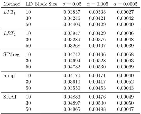
Table 1.1. Empirical Type I Error Rates for Continuous Trait
Type I error rates for each LD block size (10,30,50 SNPs) are shown for significance levelsα = 0.05,0.005,and 0.0005. The LD blocks were randomly selected from chromo-somes 12 through 22. Each error rate is based on 120,000 simulations using HapMap 3 CEU genotypes and sample size ofn= 1000. To calculatep-values forLRT1 andLRT2,
Method LD Block Size α= 0.05 α= 0.005 α= 0.0005
LRT1 10 0.03763 0.00352 0.00032
30 0.03885 0.00387 0.00035
50 0.04076 0.00363 0.00044
LRT2 10 0.03877 0.00438 0.00035
30 0.03272 0.00375 0.00044
50 0.03187 0.00410 0.00042
SIMreg 10 0.04762 0.00510 0.00062
30 0.04781 0.00507 0.00057
50 0.04673 0.00495 0.00062
minp 10 0.04080 0.00447 0.00036
30 0.03520 0.00392 0.00047
50 0.03413 0.00417 0.00044
SKAT 10 0.04839 0.00487 0.00056
30 0.04802 0.00504 0.00057
50 0.04727 0.00487 0.00059
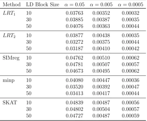
Table 1.2. Empirical Type I Error Rates for Binary Trait
Type I error rates for each LD block size (10,30,50 SNPs) are shown for significance levelsα = 0.05,0.005,and 0.0005. The LD blocks were randomly selected from chromo-somes 12 through 22. Each error rate is based on 120,000 simulations using HapMap 3 CEU genotypes and sample size ofn= 1000. To calculatep-values forLRT1 andLRT2,
t pkthresh nblocks mean nSNP med nSNP mean kb med kb
0.03 0.4 214 39.7 34.5 156407.1 97401.0 0.04 0.4 257 33.0 29.0 127973.6 74233.0 0.05 0.4 303 27.9 23.0 106706.4 58535.0 0.06 0.4 349 24.1 20.0 90508.3 50107.0 0.07 0.4 391 21.4 17.0 79899.8 43157.0 0.08 0.4 434 19.1 15.0 71153.9 38445.5 0.09 0.4 476 17.3 14.0 63755.4 34544.5 0.1 0.4 509 15.9 12.0 57941.4 31230.0 0.11 0.4 546 14.7 11.0 53051.9 29462.5 0.12 0.4 576 13.7 11.0 48744.2 27144.5 0.03 0.5 311 27.0 22.0 102424.5 62423.0 0.04 0.5 378 22.0 18.0 81595.0 42397.0 0.05 0.5 447 18.3 14.0 67274.5 37246.0 0.06 0.5 512 15.6 12.0 56340.3 30177.0 0.07 0.5 549 14.2 11.0 50612.6 28566.0 0.08 0.5 578 13.0 10.0 46111.5 25046.0 0.09 0.5 612 11.9 10.0 41786.1 24080.0 0.1 0.5 656 10.8 9.0 37566.3 21999.0 0.11 0.5 669 10.2 8.0 35269.6 19748.0 0.12 0.5 689 9.5 8.0 32706.1 19052.0 0.03 0.6 426 18.7 15.0 68452.4 38602.0 0.04 0.6 497 15.3 12.0 54644.3 30878.0 0.05 0.6 547 13.1 10.0 46058.2 26588.0 0.06 0.6 576 11.8 10.0 40764.9 24341.5 0.07 0.6 601 10.6 8.0 36244.5 21867.0 0.08 0.6 592 10.1 8.0 34050.2 20778.5 0.09 0.6 601 9.4 8.0 30949.2 19359.0 0.1 0.6 592 8.8 7.0 28767.4 18732.5 0.11 0.6 572 8.4 7.0 27572.7 17193.0 0.12 0.6 543 8.2 7.0 27015.1 16757.0 0.03 0.7 543 12.8 10.0 44181.6 27027.0 0.04 0.7 557 11.3 9.0 38279.8 24405.0 0.05 0.7 555 10.2 8.0 34534.8 22031.0 0.06 0.7 542 9.4 8.0 30936.6 19317.0 0.07 0.7 526 8.9 7.0 29247.6 18904.5 0.08 0.7 507 8.3 7.0 26561.4 16864.0 0.09 0.7 481 7.9 6.0 24805.1 16178.0 0.1 0.7 449 7.6 6.0 24009.6 15692.0 0.11 0.7 415 7.4 6.0 23566.1 15263.0 0.12 0.7 398 7.2 6.0 22440.9 14991.0 0.03 0.8 620 9.1 7.0 29836.7 18915.5 0.04 0.8 611 8.0 6.0 25871.9 16500.0 0.05 0.8 574 7.4 6.0 23705.7 14950.5 0.06 0.8 546 6.9 5.0 21179.4 13785.0 0.07 0.8 507 6.5 5.0 20089.7 12772.0 0.08 0.8 472 6.3 5.0 18925.9 12160.5 0.09 0.8 432 6.2 5.0 18261.4 11800.5 0.1 0.8 398 6.1 5.0 17950.8 10918.0 0.11 0.8 364 6.0 5.0 17381.5 10423.5 0.12 0.8 340 5.9 5.0 17384.7 10544.0
Table 1.5. For several combinations of the LD block algorithm parameters t and pk
Chapter 2
Mantel Statistics and Siemiatycki
Moments
2.1
Introduction
The basic idea of trait-similarity approaches is that, for genomic regions harboring
loci that affect a trait, individuals with similar genotypes/haplotypes should have more
similar traits. Therefore, as a nonparametric alternative to the likelihood-based testing
in Chapter 1, we consider a statistic that directly correlates genetic and trait
similar-ity. The Mantel statistic20 for space-time clustering was proposed to identify disease
clustering by testing for a positive relationship between temporal distance and spatial
distance between all pairs of individuals in a sample. The statistic has been widely used
and the paper has more than 5200 citations in the Science Citation Index as of 2013.
Hypothesis testing using Mantel statistics has usually required direct sampling from the
permutation distribution. However, formulas for the exact first four moments of the
permutation distribution are available,27 and moment-based density approximations