OnePC: A portable software for parallel genetic algorithms used in optimization problems

(1)

78



Abstract—OnePC is a software entirely written in ANSI C++ using the QT library to be portable. The software implements parallel genetic algorithms that are based to a novel algorithm to tackle the global optimization problem. The proposed algorithm contains an enhanced stopping rule and a periodical application of a local search procedure. Also, the software contains a script language to assist the programmers. The article introduces the software and the underlying algorithm as well as some experimental results.

Index Terms—: Genetic algorithms, Global optimization, Parallel Computing, Programming tool

I. INTRODUCTION

The common problem of estimating the global minimum of a multi - dimensional function is given as

𝑥 = arg min 𝑓 𝑥 𝑥∈𝑆 where𝑆 is a subset of 𝑅𝑛_{and is defined by:}

𝑆 = 𝑎1, 𝑏1 × 𝑎2, 𝑏2 × ⋯ 𝑎𝑛, 𝑏𝑛

This problem appears in many scientific areas such as [1]-[2], chemistry [3]-[4], economics [5] etc. One common technique to tackle this is the naturally inspired method of genetic algorithms [6]. Genetic algorithms have been used in a many fields [7]-[9] and they have many advantages such as:

 Adaptation in every problem

 Requirement for the objective function only and not for gradient functions

 They can be parallelized easily

The most frequent model for parallel genetic algorithms is the server - client model, such as the so called Island model [10]-[11], where clients run a a local genetic algorithm and the server collects information from the clients and occasionally distributes information to them, such as the best discovered minimum.The proposed software named OnePC implements a client - server model for parallel genetic algorithms with some advanced features such as:

1. A modified stopping rule. This termination rule has been proposed also in a recent work [12] and it is

general enough to be adapted in any genetic algorithm.

2. A periodical application of a local search procedure.

3. Exchange of best chromosomes between clients.

The proposed software has been written entirely in ANSI C++ using the Qt library freely available from http://qt.io in order to be portable in any operating system.

The rest of this article has as follows: in section II a detailed description of the method is given, in section III full documentation of the software is provided, in section IV some experiments that outline the usability of the software are listed and finally in section V some conclusions are presented accompanied with some guidelines for future research.

II. METHOD DESCRIPTION

A. Server algorithm

The machine denoted as server is responsible to gather from client machines the corresponding best discovered values. The algorithm executed on server is outlined below.

Initalization Step

1. Set𝑔𝑚= ∞

2. Set N, the number of clients

Check Step

1. If all clients have finished then

a. Report𝑔𝑚 as the global minimum

b. Terminate

2. Endif

Loop Step

1. For i=1...N Do

a. Obtain the minimum 𝑔𝑖 from the client i b. If 𝑔𝒊< 𝑔𝑚then 𝑔𝒎= 𝑔𝑖

2. EndFor

3. GotoCheck Step

OnePC: A portable software for parallel

genetic algorithms used in optimization

problems

Ioannis G. Tsoulos,

(2)

Volume 6, Issue 6, June 2017

B. Client algorithm

On each client a genetic algorithm with the termination rule described in [12] accompanied with an additional local search operator is applied. The steps of the algorithm are given below:

1. Initialization Step

a. Set iter=0, where iter is the current number of generations

b. Set𝑁𝑐 the number of chromosomes c. Initialize chromosomes 𝑋𝑖, 𝑖 = 1, … , 𝑁𝑐 d. Set IMAX as the maximum number of

allowed generations

e. Set 𝑝𝒔as the selection rate and 𝑝𝑚 as the mutation rate. Both rates are in range [0,1]. f. Set 𝑓𝑙 = ∞ as the best discovered fitness. g. Set 𝐿𝐼the number of generations that

should pass before the local search procedure is applied.

h. Set 𝐿𝐶the number of chromosomes that will participate in local search procedure.

2. Termination Check. At every generation the

variance 𝜎(𝑖𝑡𝑒𝑟 )_of_𝑓_{𝑙 is calculated. If there was no} improvement of the genetic algorithm for a number of generations, then the algorithm should terminate. The stopping rule has as follows:

𝜎 𝑖𝑡𝑒𝑟 _≤𝜎 𝑙𝑎𝑠𝑡

2 𝑂𝑅 𝑖𝑡𝑒𝑟 > 𝐼𝑀𝐴𝑋 (3)

Where last denotes the generation number where 𝑓𝑙 was produced initially. If the above equation is true

thengoto Step 10.

3. Fitness calculation. Calculate the fitness 𝑓𝑖 of every chromosome of the population.

4. Genetic operators.

a. Selection procedure. The chromosomes

are sorted in descending order according to their fitness value. The first 1 − 𝑝𝑠 × 𝑁𝑐chromosomes are transferred to the next generation. The rest of the chromosomes are substituted by offsprings created through crossover procedure: For every offspring two chromosomes (parents) are selected from the old population using tournament selection. The procedure of tournament selection has as follows:A set of N>1 randomly selected chromosomes is produced and the chromosome with the best fitness value in this set is selected and the others are discarded. Having selected the parents, the offsprings𝑥 and 𝑦 are produced according to the equations 𝑥 = 𝑎𝑖 𝑖𝑥𝑖+ 1 − 𝑎𝑖 𝑥𝑖 and 𝑦 = 𝑎𝑖 𝑖𝑦𝑖+ 1 − 𝑎𝑖 𝑦𝑖 where 𝑎𝑖 are random number in the range [-0.5,1.5] as suggested in [13].

b. Mutation procedure. Mutatethe

offsprings produced during crossover with probability𝑝𝑚 . Suppose that the element i of a given chromosome x is denoted as 𝑥𝑖. The new element 𝑥′𝑖 is calculated with an equation borrowed from the popular PSO optimization method [14]:

𝑥′𝑖 = 𝑐1𝑟1 𝑥𝑖𝑏− 𝑥𝑖 + 𝑐2𝑟2 𝑥𝑖𝑙− 𝑥𝑖

where 𝑐1 and 𝑐2 are two positive constants (acceleration coefficients) , 𝑟1 and 𝑟2 are random numbers in the range [0,1], the vector 𝑥𝑏_{is a copy of the best so far} position of chromosome x and 𝑥𝑙_{is the} best discovered chromosome so far.

c. Replacethe 𝑝𝑠× 𝑁𝑐 worst chromosomes

in the population with the offsprings created by the genetic operators.

5. Set iter=iter+1

6. Local Search Step

a. If iters mod 𝐿𝐼 =0 then

i. Select randomly 𝐿𝐶 chromosomes from the genetic population and create the set 𝐿𝑆 from these chromosomes.

ii. For every chromosome 𝑋𝑖 ∈ 𝐿𝑆

1. Select randomly another

chromosome Y from the population

2. Create an offspring of 𝑋𝑖 and Y. Denote this chromosome as Z 3. Obtain the fitness f(z) of

the chromosome Z 4. If 𝑓 𝑧 < 𝑓 𝑥𝑖 then

𝑋𝑖 = 𝑍

iii. EndFor

b. Endif

7. Obtainthe best value in the population, denoted as𝑓𝑙 for the corresponding chromosome 𝑥𝑙.

8. Send 𝑥𝑙, 𝑓𝑙 to the server machine. 9. Goto step 3.

10. Send 𝑥𝑙, 𝑓𝑙 to the server machine.

11. Terminate.

III. SOFTWARE DOCUMENTATION

In this section a detailed description of the main parts of the software is provided. More detailed information about the software that includes some screenshots can be found in the URL http://itsoulos.teiep.gr/OnePCSite/index.html. Also a last copy of the software is provided in https://github.com/itsoulos/OnePC

A. User provided functions

The user should code the objective function in C++. The C++ files should have the following command before any function in the file

extern “C” {

and the line

}

after them. The user should supply the following functions: 1. getdimension().It is an integer function which

returns the dimension of the objective function. 2. getleftmargin(left).It is an integer function which

(3)

80

3. getrightmargin(right).It is an integer function which returns the dimension of the objective function.

4. funmin(x). It is an integer function which returns the dimension of the objective function.

As an example consider the Rastrigin function: 𝑓 𝑥1, 𝑥2 = 𝑥12+ 𝑥22− cos 18𝑥1 − cos 18𝑥2 The code for this objective function is shown in Fig. 1 Also the user may optionally provide the following functions:

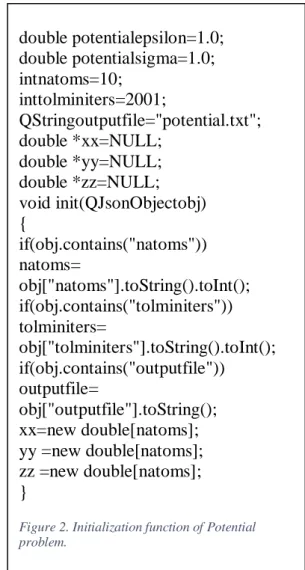
1. void init(QJsonObject params). This function initializes the objective problem and it is not mandatory. In params parameter user stores some useful parameters for the problem. The user should use the include directive #include <QJsonObject> at the beginning of the file. As an example consider the initialization function for the problem of energy potential shown in Fig. 2, where some critical parameters of the objective function are initialized through the init() function.

2. double done(double *x). This function should be called at the end of optimization. The double parameter x is the vector of global minimum discovered by the optimization process. The function should return the final value of the objective function. It is useful when a local optimization algorithm is required at the end of the optimization of in the neural network case, where the neural network should be applied to the test set. The objective problem is written in ANSI C++ and it should build as a shared library. The use can use any programming tool to achieve that, but the best choice is to use Qt build environment for that. The project file is used in Qt programming environment to build the associated project. In our case is used to build the optimization function. An example for building the potential optimization function is illustrated in Fig 3.

B. The program OnePCServer

Installation

The user should issue the following commands to build the program OnePC Client (under some Unix machine):

1. Download the code (OnePcClient.tar.gz) 2. gunzip OnePcClient.tar.gz

3. tar xfv OnePcClient.tar 4. cd OnePcClient 5. qmake . 6. make

User Interface

The graphical interface of the program is written entirely in Qt and it contains for main tabs:

1. Info tab. The tab contains information about the machine running the server. The most important information from this tab is the IP of the server and the port where it is running. This information should be used by the clients that want to connect to genetic server. Also, the user can load OneScript programs using the button LOAD SCRIPT.

2. Clients tab. This is the tab where the user can start the parallel genetic algorithm by pressing the button Run Experiment. This button sends on every client the objective function. The function will be sent in the corresponding format of every client depending

of the running operating system. Afterwards each client starts the genetic algorithm. The Clients tab displays also the following information for every client:

a. Name of the client

b. Operating system of the client

c. Status of the client (running, waiting, terminated, paused)

d. Discovered global minimum from the client

3. Problems tab. The information about the stored objective problems is outlined in this tab. This information is stored in a sqlite3 database named gaserver.db3 in the same folder with the running server. The user can load compiled objective problems in shared library format from the hard disk and he can also change or add parameters to the objective problem through the relevant dialog.

4. Messages tab. This tab displays debug information

for every client as well as about the status of the running server.

C. The program OnePCClient

Installation

The user should issue the following commands to build the program OnePC Client (under some Unix machine):

1. Download the code (OnePcClient.tar.gz) 2. gunzip OnePcClient.tar.gz

3. tar xfv OnePcClient.tar 4. cd OnePcClient 5. qmake . 6. make

User interface

The graphical application is written entirely in Qt in order to be portable. Nevertheless, the user can start the client in command line mode by starting the executable with the command line –gui=no. The graphical application is organized in three tabs:

1. Connection tab. In this tab the user should supply the ip of the server in the Host textfield as well as the running port. Without this information the client cannot connect to the server. Also, the user can provide a name for the client in order to distinct them from other running clients.

2. Run tab. Under Run tab the user can modify some

of the most critical parameters of the genetic algorithm such as chromosomes, generations etc. Also, the user can monitor the progress of the genetic algorithm during the execution of the algorithm.

3. Messages tab. Some debug information is

displayed in this tab.

Command line options

The user can use command line arguments for the application.

1. –generations=g. The integer value g specifies the maximum number of generations allowed for the genetic algorithm. The default value is 200. 2. –chromosomes=c. The integer value c specifies the

(4)

population. The default value for this parameter is 200.

3. –selectionrate=s. The double parameter s

determines the selection rate for the genetic algorithm. The default value is 0.90 (90%), which means that 90% of the population will be copied intact to the next generation.

4. –mutationrate=m. The double parameter m

determines the mutation rate used in genetic algorithm. The default value is 0.05 (5%).

5. –serverip=s. The string parameter s specifies the ip server of the OnePC server.

6. –serverport=p. The integer parameter p specifies the port of the OnePC server.

7. –gui=b. The boolean value b can specifies if gui will be used for the client. If b is yes or true the gui will be used otherwise it will not.

8. –seed=s. The integer parameter s specifies the seed for the random generator.

9. –machinename=name. The string parameter name

specifies the name of the client that will be displayed under tab Clients in OnePC server.

10. –parallelchromosomes=c. The integer parameter c

specifies the number of chromosomes that will be exchanged between this client and the other clients in the parallel population. The default value for this parameter is 10.

11. –localsearchchromosomes=c. The integer

parameter c specifies the amount of chromosomes that will take part into local search step of the genetic algorithm. The default value for this

parameter is 20.

12. –localsearchgenerations=g. The integer parameter

g specifies the amount of generations that will be executed before the local search step of the genetic algorithm. The default value for this parameter is 50.

D. The language OneScript

The language OneScript can be used to simplify the execution of a series of problems in OnePC without the interference of the programmer. The commands can be written using capital or lowercase letters. For the time being the language has a simple set of commands which are:

1. SET PROBLEM name. Sets the current problem to name.

2. SET PARAMETER paramName paramValue. Change the value of the parameter paramName to paramValue.

3. RUN. Executes the current problem using the attached clients.

4. PRINT FILE. Print the current global minimum to file FILE.

As an example of a script in OneScript consider the program listed in Fig. 4 used to set the objective problem to SINU.

# include <math.h>

extern "C"

{

intgetdimension()

{

return 2;}

void getleftmargin(double *x)

{

x[0]=-1;

x[1]=-1;

}

void getrightmargin(double *x)

{

x[0]=1;

x[1]=1;

}

double funmin(double *x)

{

return

x[0]x[0]+x[1]x[1]-cos(18.0*x[0])

-cos(18.0*x[1]);

}

double potentialepsilon=1.0;

double potentialsigma=1.0;

intnatoms=10;

inttolminiters=2001;

QStringoutputfile="potential.txt";

double *xx=NULL;

double *yy=NULL;

double *zz=NULL;

void init(QJsonObjectobj)

{

if(obj.contains("natoms"))

natoms=

obj["natoms"].toString().toInt();

if(obj.contains("tolminiters"))

tolminiters=

obj["tolminiters"].toString().toInt();

if(obj.contains("outputfile"))

outputfile=

obj["outputfile"].toString();

xx=new double[natoms];

yy =new double[natoms];

zz =new double[natoms];

}

(5)

82

QT -= gui TARGET = potential TEMPLATE = lib

DEFINES += POTENTIAL_LIBRARY SOURCES += potential.cpp tolmin.cc HEADERS += potential.hpotential_global.h unix {

target.path = /usr/lib INSTALLS += target }

Figure 3. Project file to build the potential objective function.

IV. EXPERIMENTS

The method was tested on some test functions from the relevant literature as well as on the Lennard Jones potential problem. The results are compared against the well-known software for parallel computation called GALib-mpi[18]. The experiments were performed 30 times using different seed for the random generator each time and averages were taken. The number of chromosomes was set to 200 and the maximum number of allowed generations was set to 2000.

A. Experiments on Test Function

The following test functions were used in the experiments: 1. Gkls. f(x)=Gkls(x,n,w) is a function with w local

minima described in [19], 𝑥 ∈ −1,1 𝑛_{, 𝑛 ∈} [2,100]. In the conducted experiments the cases of n=2,3,4 with 50 local minima were used.

2. Test2n. The function is given by 𝑓 𝑥 =1

2 𝑥𝑖 4_{− 16𝑥}

𝑖2+ 5𝑥𝑖 𝑛

𝑖=1 with 𝑥 ∈

[−5,5]𝑛_{. The function has}₂𝑛_{local minima in the} specified range. In the conducted experiments the cases of n=5,6,7 was considered.

3. Sinusoidal. The function f(x) is given by 𝑓 𝑥 =

− −2.5 𝑛𝑖=1sin 𝑥𝑖− 𝑧 + 𝑛𝑖=1sin 5 𝑥𝑖− 𝑧 with 0 ≤ 𝑥𝑖≤ 𝜋 and 𝑧 =

𝜋

6. The global minimum is -3.5

4. The Chemical Equilibrium.The problem is

described in [15] and it is described by the following set of equations:

x1x2+ x1− 3x5 = 0

2x₁x₂+ x₁+ x₂x₃2_{+ R}

8x2− Rx5+ 2R10x22+ R7x2x3+ R9x2x4 = 0 2x2x32+ 2R5x32− 8x5+ R6x3+ R7x2x3 = 0

R₉x₂x₄+ 2x₄2_{+ 4Rx}

5 = 0

x1 x2+ 1 + R10x22+ x2x32+ R8x2+ R5x32+ x42− 1 + R6x3+ R7x2x3+ R9x2x4 = 0 where

𝑅 = 10

𝑅5 = 0.193

𝑅6 =

0.002596 40

𝑅7 =

0.00348 40

𝑅8 =

0.00001799 40

𝑅9 =

0.0002155 40

𝑅10 =

0.00003846 40

The corresponding objective function is the summation of the absolute values of all equations in the system i.e.

𝑓 𝑥 = 𝑓𝑖(𝑥) 𝑛

𝑖=1 The global minimum is 0.

5. The Kinematic Application. This function is

described in [15] for the inverse position problem for a six – revolute – joint problem in mechanics. The problem is provided as a system of equations:

𝑥𝑖2+ 𝑥𝑖+12 = 0

𝑎1𝑖𝑥1𝑥3+ 𝑎2𝑖𝑥1𝑥4+ 𝑎3𝑖𝑥2𝑥3+ 𝑎4𝑖𝑥2𝑥4+ 𝑎5𝑖𝑥2𝑥7 +

𝑎6𝑖𝑥5𝑥8+ 𝑎7𝑖𝑥6𝑥7+ 𝑎8𝑖𝑥6𝑥8+ 𝑎9𝑖𝑥1+ 𝑎10𝑖𝑥2+ 𝑎11𝑖𝑥3 +

𝑎12𝑖𝑥4+ 𝑎13𝑖𝑥5+ 𝑎14𝑖𝑥6+ 𝑎15𝑖𝑥7+ 𝑎16𝑖𝑥8+ 𝑎17𝑖 = 0

Where 1 ≤ 𝑖 ≤ 4 and the table 𝑎𝑖𝑗 is

𝑎

=

−0.249150 0.125016 −0.635550 1.489477

1.6091354 −0.68660736 −0.1157199 0.230623 0.27942343 −0.11922812 −0.666404 1.3281073

1.4348016 −0.71994047 0.110362 −0.258645

0.0 −0.43241927 0.2907020 1.165172

0.40026384 0.0 1.2587767 −0.26908

−0.80052768 0.0 −0.629388 0.53816

0.0 −0.86483855 0.581404 0.582585

0.07405 −0.03715727 0.195946 −0.208169

−0.083050 0.0354368 −1.228034 2.686832

−0.38615961 0.085383482 0.0 −0.699103

−0.75526603 0.0 −0.079034 0.3574441

0.50420168 −0.039251967 0.026387 1.249911

−1.0916287 0.0 −0.057131 1.467736

0.0 −0.43241927 −1.1628081 1.165172

0.04920729 0.0 1.2587767 1.0763397

0.04920729 0.01387301 2.162575 −0.696868

The corresponding objective function is the summation of the absolute values of all equations in the system i.e.

6. The Combustion Application. This problem is also

described in [15] as a series of equations:

𝑥2+ 2𝑥6+ 2𝑥9𝑥10− 10−5 = 0

𝑥3+ 𝑥8− 3 × 10−5 = 0

𝑥1+ 𝑥3+ 2𝑥5+ 2𝑥8+ 𝑥9+ 𝑥10− 5 × 10−5 = 0

𝑥4+ 2𝑥7− 10−5 = 0

0.5140437 × 10−7_𝑥

5− 𝑥12 = 0 0.1006932 × 10−6_𝑥

6− 2𝑥22 = 0 0.7816278 × 10−15_𝑥

7− 𝑥42 = 0 0.1496236 × 10−6_𝑥

8− 𝑥1𝑥3 = 0 0.619441 × 10−7_𝑥

9− 𝑥1𝑥2 = 0 0.2089296 × 10−14_𝑥

10− 𝑥1𝑥22 = 0 SET PROBLEM sinu

SET PARAMETER dimension 16 RUN

PRINT /home/user/log_sinu16.txt

(6)

Again, the corresponding objective function is the summation of the absolute values of all equations in the system i.e.

The results from the applications of OnePC and Galib to the problems above are presented in TableI for two processors, in TableII for four processors and in TableIII for eight processors. The cells denote average number of generations and the figures in parentheses denote the fraction of runs that located the global minimum and were not trapped in one of the local minima. Absence of this fraction denotes 100% success in locating the global minimum. In all tables the column FUNCTION denotes the function name, the column GAlib denotes the results from the application of GALIB and the column ONEPC denotes the results from the application of the proposed software.

As we can deduce from the experimental results the proposed software seems to require lower number of generations than GAlib to discover the global minimum. Also the fraction of runs that discovered the global minimum is higher than GAlib.

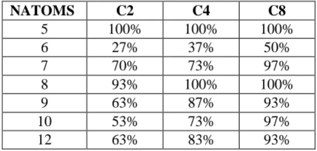
B. The case of Lennard Jones Potential

The molecular conformation corresponding to the global minimum of the energy of N atoms interacting via the Lennard-Jones potential [16] is used as a test case here. The function to be minimized is given by:

𝑉𝐿𝐽 𝑟 = 4𝜖 𝜎 𝑟

12 − 𝜎

𝑟 6

The function is minimized firstly with OnePC and afterwards the local search procedure Tolmin (a BFGS variant of Powell [17]) is used to enhance the detected minimum. Success rates of discovering the global minimum by GAlib are presented in TableIV and success rates obtained by the proposed method are presented in Table V. Again in most cases the fraction of runs that discovered the global minimum is higher than GAlib.

V. CONCLUSIONS

A portable software for global optimization was introduced with the following features:

1. It can be installed in most operating systems. 2. There is no need for parallel libraries such as

OpenMPI[20].

3. The system continues to work even if some of the nodes have lost connection.

4. The clients can operate with or without GUI. 5. The user can control the initialization parameters

of the objective problems through the init() procedure.

6. The server can use a script language to control the optimization procedure

Future research may include:

1. Additional commands for the script language of the server.

2. More advanced stopping rules.

Table IExperimental results using two processors for a series of optimization problems

PROBLEM GaLib OnePC

GKLS350 310.50 205.18

GKLS450 370.20(0.30) 393.78(0.77) GKLS550 1548.70(0.93) 569.80(0.80)

SINU16 1933.50 1633.63

SINU32 1933.57(0.90) 1644.18 SINU64 272.50(0.17) 155.68(0.17)

TEST2N4 543.60 425.02

TEST2N5 857.63 521.22

TEST2N6 1037.37 786.27

TEST2N7 1207.90(0.93) 891.7 CHEMICAL 1917.25(0.93) 1415.31 KINEMATIC 1976.37 1601.81 COMBUSTION 1865.67 1409.19

Table IIExperimental results using four processors for a series of optimization problems

GKLS350 429.93 255.58

GKLS450 424.87(0.33) 359.73(0.90) GKLS550 1322.43(0.90) 585.87 SINU16 1867.20(0.90) 1611.76 SINU32 1740.63(0.90) 1657.10 SINU64 339.50(0.23) 72.29(0.30)

TEST2N4 712.67 342.78

TEST2N5 984.57(0.97) 498.70 TEST2N6 983.47(0.90) 624.65 TEST2N7 1015.67(0.70) 957.80

CHEMICAL 1825.37 1319.69

KINEMATIC 1903.94 1644.89 COMBUSTION 1836.54 1241.43

Table IIIExperimental results using eight processors for a series of optimization problems

GKLS350 418.17 224.49

GKLS450 626.40(0.40) 373.13 GKLS550 1291.00(0.83) 592.63 SINU16 1933.26(0.93) 1642.59 SINU32 1933.63(0.87) 1678.78 SINU64 373.87(0.23) 55.38(0.67)

TEST2N4 461.77 375.70

TEST2N5 947.70(0.97) 506.12 TEST2N6 1092.13(0.93) 629.29 TEST2N7 1097.43(0.73) 883.76

(7)

84

KIMEMATIC 1945.60 1636.10

COMBUSTION 1875.49 1252.35

Table IVSuccess rate results for the Potential problem with GaLib

NATOMS C2 C4 C8

5 100% 100% 100%

6 27% 37% 50%

7 70% 73% 97%

8 93% 100% 100%

9 63% 87% 93%

10 53% 73% 97%

12 63% 83% 93%

Table VSuccess rate results for the Potential problem with OnePC

NATOMS C2 C4 C8

5 100% 100% 100%

6 100% 100% 100%

7 80% 100% 100%

8 60% 80% 100%

9 70% 100% 100%

10 40% 80% 90%

12 100% 100% 100%

REFERENCES

[1] P. O. Yapo, H. V. Gupta and S. Sorooshian, “Multi-objective global optimization for hydrologic models,” Journal of Hydrologyvol 204, pp. 83-97, 1998.

[2] Q. Duan, S. Sorooshian and V. Gupta, “Effective and efficient global optimization for conceptual rainfall-runoff models,”Water Resources Researchvol 28, pp. 1015-1031, 1992.

[3] D. J. Wales and H. A. Scheraga, “Global Optimization of Clusters, Crystals, and Biomolecules,” Science vol27, pp. 1368-1372, 1999. [4] P.M. Pardalos, D. Shalloway and G. Xue, “Optimization methods for

computing global minima of nonconvex potential energy functions,” Journal of Global Optimization vol. 4, pp. 117-133, 1994.

[5] Zwe-Lee Gaing, “Particle swarm optimization to solving the economic dispatch considering the generator constraints,” IEEE Transactions on Power Systems vol. 18, pp. 1187-1195, 2003.

[6] D.E. Goldberg and J. H. Holland, “Genetic Algorithms and Machine Learning,” Machine Learning vol. 3, pp. 95-99, 1988.

[7] J.J. Grefenstette, R. Gopal, B. J. Rosmaita and D. Van Gucht, “Genetic Algorithms for the Traveling Salesman Problem”, In: Proceedings of the 1st International Conference on Genetic Algorithms, pp. 160 - 168, Lawrence Erlbaum Associates, 1985.

[8] P. Kaelo and M.M. Ali, “Integrated crossover rules in real coded genetic algorithms,” European Journal of Operational Research vol. 176, pp. 60-76, 2007.

[9] T. Prasad and N. Park, “Multiobjective Genetic Algorithms for Design of Water Distribution Networks,” J. Water Resour. Plann. Manage. vol. 130, pp. 73-82, 2004.

[10] A. L. Corcoran and R. L. Wainwright,” A parallel island model genetic algorithm for the multiprocessor scheduling problem,” SAC '94 Proceedings of the 1994 ACM symposium on Applied computing, pp. 483-487, 1994.

[11] D. Whitley, S. Rana and R. B. Heckendorn, “Island model genetic algorithms and linearly separable problems,” Evolutionary Computing Volume 1305 of the series Lecture Notes in Computer Science, pp 109-125, 2005.

[12] I.G. Tsoulos, “Modifications of real code genetic algorithm for global optimization,” Applied Mathematics and Computation vol. 203, pp. 598-607, 2008.

[13] Z. Michaelewicz, Genetic Algorithms + Data Structures = Evolution Programs. Springer - Verlag, 1996.

[14] J. Kennedy and R.C. Eberhart, “The particle swarm: social adaptation” in information processing systems, in: D. Corne, M. Dorigo and F.

Glover (eds.), New ideas in Optimization, McGraw-Hill, Cambridge, UK, pp. 11-32, 1999

[15] C. Grosan and A. Abraham. “A new approach for solving nonlinear equations systems.” IEEE Transactions on Systems, Man, and Cybernetics–Part A: Systems and Humans vol.38, pp. 698– 714, 2008. [16] J.E. Lennard-Jones, “On the Determination of Molecular Fields,”Proc.

R. Soc. Lond. A, vol. 106: pp. 463–477, 1924.

[17] M.J.D Powell, “A Tolerant Algorithm for Linearly Constrained Optimization Calculations,” Mathematical Programming vol. 45, pp 547, 1989

[18] M. WALL “GAlib: A C++ library of genetic algorithm components.” Mechanical Engineering Department, Massachusetts Institute of Technology 87: pp.54, 1996.

[19] M. Gaviano , D.E. Ksasov, D. Lera and Y.D. Sergeyev, “ Software for generation of classes of test functions with known local and global minima for global optimization,” ACM Trans. Math. Softw. Vol. 29, pp. 469-480, 2003.