Teaching Least Squares in Matrix Notation

Teaching Least Squares in Matrix Notation

Guglielmo Monaco

, Aniello Fedullo

1_{Department of Chemistry and Biology ”A. Zambelli”, University of Salerno, Italy}

[email protected]

2_{Department of Physics ”E. R. Caianiello”, University of Salerno, Italy}

[email protected]

Receivedon: 30-05-2017. Acceptedon: 27-06-2017. Publishedon: 30-06-2017

doi:10.23755/rm.v32i0.335

c

G. Monaco and A. Fedullo

Abstract

Material for teaching least squares at the undergraduate level in matrix notation is reported. The weighted least squares equations are first derived in matrix form; equivalence with the standard results obtained by standard algebra are then given for the weighted average and the simplest linear re-gression. Indicators of goodness of fit are introduced and interpreted. Even-tually a basic equation for resampling is derived.

Keywords: coefficient of determination, weighted sample mean, resam-pling, undergraduate education.

2010 AMS subject classifications: 62J05.

1

Introduction

Statistics is a never missing topic in first degree courses of scientific programs. Very soon, often at the second year undergraduate, the basic knowledge of random variables and distributions, is complemented by the simple linear regression, as a necessary tool for the interpretation of experimental data gathered in the labo-ratories. Indeed, the critical practice of linear regressions often forms students’ basic awareness of data analysis. The advent of powerful and handy softwares on the one hand has reduced the effort required to the students for accomplish-ing the needed calculations, on the other hand has given them the possibility to easily perform more advanced statistical analyses [1, 2], which they cannot really understand on the grounds of the course. One of simplest of such more advanced analyses is the consideration of more regressors, the starting point of multivariate data analysis [3]. Although a specific course at the last undergraduate or first grad-uate year can be much profitable, we experienced that, provided the students have a basic knowledge in linear algebra, the generalized least squares can be thought at the second year undergraduate with reasonable appreciation from the class. Reference textbooks on the matter, seemingly more diffused in the community of econometrics [5] than in that of experimental sciences [6], are not missing. However, we needed to compact some fundamental concepts and equations, and still convince the students that the more general matrix form of the least squares allows to easily retrieve the results obtainable with standard algebra. Thus, we prepared the following material, and we presented it effectively in a 12 hours module together with numerical exercises. Although our lessons obviously have a significant overlap with reference textbooks, the revised simple linear regression and the introduction of the (adjusted) weighted coefficient of determination are not easily retrieved from any of the textbooks known to us.

2

Matrix Form of the Weighted Least Squares

We consider n measures {y1, y2, ..., yn} and for each of them, say the i-th

one, the regressors {xi1, xi2, ..., xip}, here assumed constant, which are generally

coming from different associated measures. We will assume that for each measure the first regressor equals one,xi1 = 1, in order to take into account the so called

intercept. The linear regression model connects the above quantities by

yi = p

X

j=1

where β1, β2, ..., βp are the parameters to be estimated andε1, ε2, ..., εn are

ran-dom errors, assumed independent and possibly normally distributed, with mean0 and standard deviationsσ1, σ2, ..., σn. Ordinary least squares (OLS) and weighted

least squares (WLS), also called homoskedastic and heteroskedastic regressions, are the names used to distinguish the special case of equal values for all standard deviations from the case of different values. The equations for WLS of course also apply to the special OLS case.

Dividing eq. 1 byσi, i.e. givenzi := y_σi_i, qij := xij

σi, ςi :=

εi

σi, and using the

matrix notation, the model is written as

z = Qβ+ς, (2)

or, equivalently,

W12y = W 1

2Xβ+W 1 2,

where W is a diagonal matrix whose elementsWii := wi = σ−i 2 are known as

statistical weights,zandβare column matrices ofnandpelements, respectively,

Qis a matrix of dimensionn×p. It should be noticed thatQβ is the expectation value ofz, i.e. Qβ =< z >.

Under these hypotheses the least squares method gives an estimate of the model parameters by the minimization with respect toβof the functional

SS:=ςTς = (z−Qβ)T(z−Qβ) (3)

= (z−Qβ)T_{(z−Qβ) = z}T_z−2βT_QT_z+βT_QT_{Qβ, (4)}

where it has been considered thatβTQTz =zTQβ.

The estimates of the parameters by the least squares method are the solutions of the equations ∂SS_∂β

i = 0, fori = 1,2, ..., p, one for each model parameter. The

computation of the derivative with respect to the vector of the parameters gives:

−QTz+QTQβ= 0, (5)

whose solution

ˆ

β =V QTz (6)

is, by definition, the least squares estimator of β, where V := C−1_{, and}

We note that βˆ is an unbiased estimator ofβ, indeed form eqs. 2 and 6 we have

<β >ˆ =V QT < z >=V QTQβ =V Cβ =β. (7) An unbiased behavior also characterizes the weighted sample mean. Indeed, eq. 5 for β = ˆβ gives QT_{z = Q}T_{zˆwhich, rewritten in the original variables, is}

XT_{W y = X}T_{Wyˆ. From this and from the initial hypothesisx}

i1 = 1, for anyi,

one gets P

iwiyi =

P

iwiyˆi, which divided by

P

iwi shows that the weighted

sample mean of the fitted values equals the weighted sample mean of the mea-sures:

¯

yw = ˆyw. (8)

Givenδ:= ˆβ−β from eqs. 6 and 7 one gets

δ = V QTς, (9)

which allows to easily compute the covariance matrix of the parameters, showing that it coincides withV

< δδT >=V QT < ςςT > QV =V QTIQV =V,

whereIdenotes the identity matrix.

The standard deviations of the estimators of the parameters are given by the square roots of the diagonal elements ofV.

Using the fitted values, one can write

z = ˆz+ (z−zˆ) =Qβˆ+e,

where e is known as the vector of residuals, whose analysis is object of much concern in literature.

The fitted values are often written as ˆ

z =Qβˆ=QV QTz =:Hz, (10)

where we have introduced the symmetric matrixH, which is known as hat matrix as it ’puts the hat on z’. This matrix is readily verified to be idempotent, H2 ₌

QV QTQV QT = H, a feature which readily allows to demonstrate the useful property of orthogonality of residuals and fitted values:

(z−zˆ)Tzˆ=zT(I−H)Hz= 0.

SSE :=minβSS=eTe,

the expansion 4, withς in place ofz andδin place ofβ, can be rewritten as:

SSE = (ς−Qδ)T(ς −Qδ) = ςTς−2δTQTς +δTCδ=ςTς−δTCδ,

where we have considered thatQTς =Cδthanks to eq. 9.

GivenSSR := δTCδ, which asSS andSSE is non-negative, the preceding equation becomes

SSE=SS−SSR

whose interpretation is that the error in the estimation of the parameters, yielding a nonzeroSSR, reduces the sum of squaresSSwhich could have been computed with the expectation valuehzi=Qβ.

The average ofSSEcan be easily computed considering thatδT_{Cδ=T r}

δδT_C , and then

hSSEi = ςTς−T rδδTC=n−T r(V C) = n−p,

known as the number of degrees of freedom, denoted byν.

Notation. In the followingsxx,w,Sxx,wesxy,windicate respectively the sample

variance, sum of squares and weighted covariance, defined from the weighted sample meany¯w :=

P

iwiyi

P

iwi in analogous manner to the corresponding unweighted

means. We recall that their expressions aresxx,w =x2w−x¯2w,Sxx,w =sxx,w

P

iwi

esxy,w=xyw−x¯wy¯w, wherexy:= (x1y1, ..., xnyn).

3

Indicators for the Goodness of Fit

Besides reporting the best-fit parameters and the resulting fitted values, it is customary to give compact indicators of the goodness of fit.

A method which is widely used in the analysis of experimental data consists in the chi-squared test: the hypothesis that the model is correct is not rejected, at the appropriate level of significance, if SSE assumes values close to hSSEi, i.e., for any number of parameters, ifχ2

r = SSE

ν is close to1. Values ofχ

2

r larger

or smaller than 1 are then considered as indicators of a poor fit or, respectively, overfitting.

A different approach considers weighted sample means. Defining theweighted coefficient of determination R2

coefficient syy,wˆ

√

syy,wsyˆy,wˆ between datayand fitted values yˆ= X

ˆ

β and thus limited by0≤R2

w ≤1, one has that

1−R_w2 = SSE

Syy,w

= see

syy,w

, (11)

showing that R2

w = 1iff SSE = 0, i.e. iff all residuals are zero. Therefore the

greater the value of R_w2 the better the agreement. Eq. 11 can be proven thanks to the orthogonality relation discussed above. The vector yww

1

2, where w 1 2 is a

column vector of elements w

1 2

i , is orthogonal to the vector of residualsz−zˆ, by

virtue of eq. 8. Therefore the orthogonality of residuals and fitted values, eq. 2, still holds if the fitted values are translated byyww

1

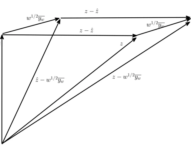
2. The vector relationship

z−yww

1

2 = (ˆz−y_ww 1

2) + (z−zˆ), (12)

graphically sketched in Figure 1, allows to assess that

Syy,w =Syˆy,wˆ +SSE, (13)

whose interpretation is that Syˆy,wˆ /Syy,w is the fraction of variability of the data

explained by the knowledge of Q, i.e. by the regression, and SSE/Syy,w is the

unexplained one, i.e. that coming from errors. Still from eq. 12 one gets

Syy,wˆ = (ˆz−yˆww

1

2)T(z−y_ww 1

2) = (ˆz−yˆ_ww 1

2)T(ˆz−yˆ_ww 1

2) =S_yˆy,wˆ (14)

and then

R2_w = S

2 ˆ

yy,w

Syˆy,wˆ Syy,w

= Syˆy,wˆ

Syy,w

. (15)

Insertion of eq. 15 in eq. 13 readily gives eq. 11.

In order to discourage the introduction of models too complicated for the data examined, it has been introduced the adjusted determination coefficient

R2_a= 1−(1−R2_w)n−1

n−p,

obtained substituting the unbiased variances in the rhs of eq. 11.

It often happens that standard deviations of experimental data are only ap-proximately known. A common assumption is that the standard deviations σiare

w

_y

w

ˆ

z

ˆ

z

−

w

y

z

−

w

1/2

_y

w

z

w

_y

w

z

−

z

ˆ

z

−

z

ˆ

Figure 1: The residualsz−zˆare orthogonal to both the estimateszˆand the vector

yww

of k leads to a good fitting for the model, χ2

r should be close to ν. Using this

value, one gets

ν =

n

X

i=1

(yi−yˆi)2

k2_σ˜2

i

,

and a trial value forkis obtained as

k = s

1

ν

P

(yi−yˆi)2

˜

σ2

i

.

4

Basic Applications

4.1

(Weighted) mean

The modely =β1+εhas ann×1matrix of relative regressors, whosei-th element is

qi1 =w 1 2

i

Application of eq. 7 soon gives as the best fit parameter the weighted mean

ˆ

β =V Qz = P

iwiyi

P

iwi

= ¯yw

and its variance is the sum of the weights: σ2

β =V11=

P

iwi.

4.2

WLS for a straight line

The standard linear regression considers the modely = a+bx. In the above notationa=β1 andb =β2 and the regressor matrix is

X =

1 1 ... 1

x1 x2 ... xn

T

The matrix of relative regressors will be then

Q=

√

w1

√

w2 ...

√

wn

√

w1x1

√

w2x2 ...

√

wnxn

T

,

z = √

w1y1

√

w2y2 ...

√

wnyn

T

,

and

C=X

i

wi

1 x¯w

¯

xw x2w

,

whose inverse gives the covariance matrix of the parameters

V = 1

Sxx,w

x2

w −x¯w

−x¯w 1

.

The standard deviations of the estimators of the parameters will be then

σaˆ

σˆ_b

= √ V11 √ V22

= _p 1

Sxx,w " q x2 w 1 # ,

and the estimated parameters will be

ˆ

a

ˆ_b

=V QTz = 1

sxx,w

x2

w −x¯w

−x¯w 1

yw xy_w = " ¯

yw− s_sxy,w_xx,wx¯w sxy,w

sxx,w

#

,

which in case of all equal weights (homoskedastic regression) have the simpler expression y¯− sxy

sxxx¯

sxy

sxx

T .

4.3

Revised simple linear regression

We now give a simplified approach for the bivariate weighted linear regres-sion: given 1 := [1 1 ... 1]T, we subtract y_w1from the data and from the fitted data and, considering thaty_w = ˆy_w =a+bx¯w, we obtain

y−y_w1=b(x−x¯w1) +ε, (16)

which, withz :=W12(y−y

w1), q:=W

1

2(x−x¯_w1)eς :=W 1

2ε, can be written

as in eq. 2,

z =bq+ς,

but here there is the single parameterbto be determined, as in the example of the weighted mean.

This means that matrixC is the scalarSxx,w readily invertible, and then V =

C−1 = _S 1

qTz = (x−x¯w1)TW(y−yw1) =Sxy,w+ yw

X

i

wi(xi−x¯w) = Sxy,w,

from eq. 6, one gets againˆb= sxy,w

sxx,w. Writing now the model asy−bx=a1+ε,

the example in 4.1 gives for the intercepty¯w−bx¯w, from where, replacingbwith

its estimator1, one finally getsaˆ= ¯yw−ˆbx¯w, as in 4.2.

It is to be considered, however, that this simplification leads to loose informa-tion on the covariance of theaandbparameters, which should then be recoverex post(Appendix).

4.4

Resampling and the Best-fit Parameters

A remarkable representation of thepbest-fit parameters can be obtained if one tries to determine them from the n_p p-elements subsets of the original set of n

measures [4]. LetS(s)be ap×nmatrix obtained from then×nidentity matrix,

upon selecting the p rows whose indices form subsets, withs = 1, . . . n_p. Let alsoM[k|v]_{be the matrix obtained from matrixM upon replacing itsk-th column}

with vectorv.

For anyp-elements subsets, the data needed for the WLS are stored in vector

z(s) =S(s)zand the square matrixQ(s)=S(s)Q; the best-fit parameters are

ˆ

β(s) =Q−_(s1₎z(s) =X₍−_s1₎W

−1/2 (s) W

1/2

(s) y(s) =X

−1

(s)y(s), (17)

which shows that, forpmeasures, WLS and OLS give the same results. Use of Cramer’s rule on eqs. 5 and 17 gives

ˆ

βk =

detQTQ[k|z]

detQT_Q , (18)

and

ˆ

β(s)k =

detQ[₍k_s|₎z]

detQ(s)

= detX

[k|y] (s)

detX(s)

, (19)

Use of the Cauchy-Binet theorem to expand the determinants of the equation 18 leads to

ˆ

βk =

P

sdetQ(s)detQ

[k|z] (s)

P

sdetQ(s)detQ(s)

= P

swsβˆ(s)k

P

sws

, (20)

which is the equation for a weighted average of the OLS resultsβˆ(s)kwith weights

ws = (detQ(s))2. (21)

The above representation of the best-fit parameters is the starting point for robust modifications of WLS, where the basic idea is to exclude from the mean the more extreme values ofβ(s)k[7].

5

Conclusions

The least squares method, a fundamental piece of knowledge for students of all scientific tracks, is often introduced considering the simple linear regression with only two parameters to be determined. However, the availability of ever more large data sets prompts even undergraduate students to a sounder and wider knowledge of linear regression. Here, we have used the linear algebra formal-ism to compact the main results of the least squares method, encompassing ordi-nary and weighted least squares, goodness of fit indicators, and eventually a basic equation of re-sampling, which could be used to stimulate interested students in an even broader knowledge of data analysis. The compactness of the equations reported above allow their introduction at the undergraduate level, provided that basic linear algebra has been previously introduced.

Acknowledgements

References

[1] R.J. Carroll and D. Ruppert. Transformation and weighting in regression. Chapmand and Hall, 1988.

[2] G. Casella and R.L. Berger. Statistical inference. Cengage Learning, 2001. [3] A. J. Dobson and A. G. Barnett. An Introduction to Generalised Linear

Models. Chapman and Hall, 2008.

[4] R. W. Farebrother. Relations among subset estimators: A bibliographical note. Technometrics, 27(1):85–86, 1985.

[5] W.H. Greene. Econometric Analysis. Prentice Hall, 2012.

[6] J. R. Taylor. An Introduction to Error Analysis: The Study of Uncertainties in Physical Measurements. University Science Books, 1997.

Appendix Moments ofˆaeˆb

Averages.

<ˆb >= <sxy,w>

sxx,w =

(x−x¯w1)TW <y−¯yw1>

sxx,w =

(x−x¯w1)TW <y>

sxx,w =

(x−x¯w1)TW <a1+bx>

sxx,w =

b(x−x¯w1)TW(x−x¯w1)

sxx,w =b;

<ˆa >=<y¯w >−x¯w <b >ˆ =a+bx¯w −x¯wb=a

The estimators are then unbiased.

Variances.

We shall use the following auxiliary results: i)Cov(yi, yj) =δijw−i 1

ii)V ar(¯yw) = T r(W)−1

iii)Cov(¯yw,ˆb) = 0

Givend := W(x−x¯w1), we have thatdT1 =

P

idi = 0and thenSxy,w =

dT(y−y¯w1) =dTy; ThenV ar(Sxy,w) =

P

ijdidjCov(yi, yj) =

P

id

2

iw

−1

i

=P

iwi(xi−x¯w)

2 _=S

xx,w from whichV ar(ˆb) = V ar_S(2Sxy,w)

xx,w =

1

Sxx,w.

V ar(ˆa) = V ar(¯yw)−x¯wCov(¯yw,ˆb)+ ¯x2wV ar(ˆb) =T r(W)

−1₊ ¯x2w

Sxx,w =

x2

w

Sxx,w.

.

Cov(ˆa,ˆb) = Cov(¯yw−x¯wˆb,ˆb) =Cov(¯yw,ˆb)−x¯wV ar(ˆb) = −_Sxx,wx¯w .

Proof of the auxiliary results

i)Cov(yi, yj) = Cov(a+bxi +εi, a+bxj +εj) = Cov(εi, εj) = δijσ2i =

δijwi−1.

ii)V ar(¯yw) = T r(W)−2P_ijwiwjCov(yi, yj) =T r(W)−2P_iwi =T r(W)−1

iii) T r(W)Cov(¯yw, Sxy,w) =

P

ijwidjCov(yi, yj) =

P

idi = 0 and then

Cov(¯yw,ˆb) = 0.