A NOVEL EXPERIMENTAL ANALYSIS OF THE MINIMUM
COST FLOW PROBLEM
A. Sadegheih*
Department of Industrial Engineering, University of Yazd P.O. Box 89195-741, Yazd, Iran
P.R. Drake
E-Business and Operation Management Division, University of Liverpool Management School Post Code L69 7ZH, Liverpool, U.K.
*Corresponding Author
(Received: May 10, 2008 – Accepted in Revised Form: February 19, 2009)
Abstract In the GA approach the parameters that influence its performance include population size, crossover rate and mutation rate. Genetic algorithms are suitable for traversing large search spaces since they can do this relatively fast and because the mutation operator diverts the method away from local optima, which will tend to become more common as the search space increases in size. GA’s are based in concept on natural genetic and evolutionary mechanisms working on populations of solutions in contrast to other search techniques that work on a single solution. An important aspect of GA’s is that although they do not require any prior knowledge or any space limitations such as smoothness, convexity or unimodality of the function to be optimized, they exhibit very good performance in most applications. The minimum cost flow problem is formulated as genetic algorithm and simulated annealing. This paper shows genetic algorithms and simulated annealing are much easier to implement for solving transportation problems compared with constructing mathematical programming formulations. Finally, a newempirical study for the effect of parameters on the rate of convergence of the GA and SA are demonstrated.
Keywords Linear Programming, Intelligent Optimization Techniques, Minimum Cost Flow Problem, Transportation Problem
ﻩﺪﻴﻜﭼ
ﺯﺍﺪﻧﺍ ﻞﻣﺎﺷ ﻢﺘﻳﺭﻮﮕﻟﺍ ﻱﺍﺮﺟﺍ ﺭﺩ ﺮﺛﺆﻣ ﻱﺎﻫﺮﺘﻣﺍﺭﺎﭘ ،ﻚﻴﺘﻧﮊ ﻢﺘﻳﺭﻮﮕﻟﺍ ﺭﺩﺓ ﺥﺮﻧ ﻭ ﻊﻃﺎﻘﺗ ﺥﺮﻧ ،ﺖﻴﻌﻤﺟ
ﺶﻬﺟ ﺖﺳﺍ . ﻥﺎﻜﻣ ﻱﺍﺮﺑﻚﻴﺘﻧﮊﻢﺘﻳﺭﻮﮕﻟﺍ ﺐﺳﺎﻨﻣ ﻊﻴﺳﻭﻱﻮﺠﺘﺴﺟ ﻱﺎﻫ
؛ﺖﺳﺍ ﺎﺑ ﺍﺭﻮﺠﺘﺴﺟﻢﺘﻳﺭﻮﮕﻟﺍﻦﻳﺍ ﺍﺮﻳﺯ
ﻲﻣﻡﺎﺠﻧﺍﺖﻋﺮﺳ ﻲﻣﺶﻬﺟﻞﻤﻋﻭﺪﻫﺩ
ﺤﻣﻪﻨﻴﻬﺑﻥﺎﻜﻣﺯﺍﺍﺭﻢﺘﻳﺭﻮﮕﻟﺍﺪﻧﺍﻮﺗ ﺭﻭﺩﻲﻠ
ﺪﻨﮐ ﺯﺍﺪﻧﺍﻪﻛﻲﻧﺎﻣﺯﺭﺩﻦﻳﺍﻭ ﺓ
ﺴﻣ ﺌ ﮒﺭﺰﺑ ﻪﻠ ﻲﻣ ﺭﺎﻜﺷﺁ ﺮﺘﺸﻴﺑ ،ﺩﻮﺷﺮﺗ ﺩﺩﺮﮔ
. ﻢﺘﻳﺭﻮﮕﻟﺍ ﺮﺑ ﻚﻴﺘﻧﮊ ﻱﺎﻫ ﺪﻳﺍ ﺱﺎﺳﺍ
ﺓ ﻡﺰﻴﻧﺎﻜﻣ ﻭ ﻲﻌﻴﺒﻃ ﻚﻴﺘﻧﮊ ﻱﺎﻫ
ﺏﺍﻮﺟ ﺯﺍﻲﺘﻴﻌﻤﺟ ﻱﻭﺭ ﻲﻠﻣﺎﻜﺗ ﻲﻣ ﺭﺎﻛﺎﻫ
ﺭﺩ ﻭ ﺪﻨﻨﻛ ﻚﻴﻨﻜﺗ ﺮﮕﻳﺩ ،ﻞﺑﺎﻘﻣ
ﺏﺍﻮﺟ ﻚﻳ ﺎﻬﻨﺗ ﻱﻭﺭ ﻮﺠﺘﺴﺟ ﻱﺎﻫ
) ﺩﺮﻔﻨﻣ ( ﻲﻣﻞﻤﻋ ﺪﻨﻨﻛ . ﻬﻣﺖﻳﺰﻣﻚﻳ ﻢﺘﻳﺭﻮﮕﻟﺍﺭﺩﻢ
ﺴﻣﻲﻠﺒﻗﺶﻧﺍﺩﻪﺑﺝﺎﻴﺘﺣﺍﺎﻬﻧﺁﻪﻛﺖﺳﺍﻦﻳﺍﻚﻴﺘﻧﮊﻱﺎﻫ ﺌ
ﺎﻳﻪﻠ
ﻪﻨﻴﻬﺑﺖﻬﺟﻑﺪﻫﻊﺑﺎﺗﻱﺍﺮﺑﻲﺘﻳﺩﻭﺪﺤﻣ ﺪﻧﺭﺍﺪﻧﻱﺯﺎﺳ
. ﻥﺎﺸﻧﻒﻠﺘﺨﻣﺕﺎﻋﻮﺿﻮﻣﻭﺩﺮﺑﺭﺎﻛﺭﺩﺍﺭﻲﺑﻮﺧﻱﺍﺮﺟﺍﺎﻬﻧﺁ
ﻩﺩﺍﺩ ﺪﻧﺍ . ﺴﻣ ﺌ ﻨﻳﺰﻫﺎﺑﻥﺎﻳﺮﺟﻪﻠ ﺔ
ﻲﻣ ﻢﻤﻴﻧ ﺎﺑ ﺩﺮﺳﻢﺘﻳﺭﻮﮕﻟﺍﻭﻚﻴﺘﻧﮊﻢﺘﻳﺭﻮﮕﻟﺍ ﺪﻨﻨﻛ
ﺓ ﺪﺷﻝﺪﻣﻲﺠﻳﺭﺪﺗ ﺖﺳﺍﻩ
. ﻪﻟﺎﻘﻣﻦﻳﺍ
ﻲﻣﻥﺎﺸﻧ ﻢﺘﻳﺭﻮﮕﻟﺍﻪﻛﺪﻫﺩ ﺩﺮﺳﻢﺘﻳﺭﻮﮕﻟﺍﻭﻚﻴﺘﻧﮊﻱﺎﻫ
ﺪﻨﻨﻛ ﺓ ﺵﻭﺭﻲﺠﻳﺭﺪﺗ ﻩﺩﺎﺳﻱﺎﻫ
ﺭﺩﻱﺮﺗ ﻪﻣﺎﻧﺮﺑﺎﺑﻪﺴﻳﺎﻘﻣ ﻱﺎﻫ
ﺎﺴﻣﻞﺣﻱﺍﺮﺑﻲﺿﺎﻳﺭ ﺋ ﻞﻤﺣﻞ ﻭ ﻞﻘﻧ ﺪﻧﺍ . ﺭﺩ ﻌﻟﺎﻄﻣﺖﻳﺎﻬﻧ ﺔ
ﻲﻳﺍﺮﮕﻤﻫﺥﺮﻧﻱﻭﺭﺎﻫﺮﺘﻣﺍﺭﺎﭘﺕﺍﺮﺛﺍﻱﺍﺮﺑﻱﺪﻳﺪﺟﻲﻠﻤﻋ
ﺩﺮﺳﻢﺘﻳﺭﻮﮕﻟﺍﻭﻚﻴﺘﻧﮊﻢﺘﻳﺭﻮﮕﻟﺍﺭﺩ ﺪﻨﻨﻛ
ﺓ ﺖﺳﺍﻩﺪﺷﺡﺮﺷﻲﺠﻳﺭﺪﺗ .
1. INTRODUCTION
Mathematical programming can be defined as programming and planning the best possible allocation of scarce resources. When the
transportation, power engineering, banking, education, petroleum, social problems, etc. The most important search method is the branch and bound technique which applies directly to both the pure and mixed problems. The general idea of the method is first to solve the problem as a continuous model. Cutting methods, which are developed primarily for integer linear problems, start with the continuous optimum. By systematically adding special secondary constraints, which essentially represent necessary conditions for integrality, the continuous solution space is gradually modified until its continuous optimum extreme point satisfies the integer conditions. The name cutting methods stems from the fact that the added secondary constraints effectively cut certain parts of the solution space that do not contain feasible integer points. Cutting planes does not partition the feasible region into sub-divisions, as in branch and bound approaches, but instead works with a single linear program, which is refined by adding new constraints until the new constraints solution is found. Non-linear programming problems come in many different shapes and forms. Unlike the Simplex Method for linear programming, there exists no single algorithm that will solve all of them. Instead, algorithms have been developed for various individual special types of non-linear programming problems. Two examples of non-linear programming applied to single-state network programming are: 1. the gradient search method; 2. quadratic programming.
The mathematical programming technique used in the time-phased optimization method is Dynamic Programming. Dynamic programming is a computational technique best suited to the optimization of sequential or multi-stage decision making problems. Dynamic programming converts such multi-stage decision problems into a series of single-stage decision problems, each with one or a few decision variables. Then, starting with the first stage, each stage is optimized over possible alternative feasible decisions within the stage, while taking into consideration the cumulative effect of the optimum decisions made in the previous stages. The ultimate solution of the problem is then generated from among the available stage optima.
The network problem provides a unified approach to many applications because of its general structure. The minimum cost flow problem holds a
acting on them [5]. The evaluation of the goodness of a solution is given by a fitness function that incorporates or models the feedback of the environment and asserts the adaptation of the individual. In an evolutionary algorithm the encoding abstracts the real solutions in a suitable format, while the operators handle these representations selecting the best performing solutions and randomly manipulating them, in order to find better adapted individuals. The algorithm is grounded to the real world through the feedback provided by the fitness function. Those features make evolutionary algorithms extremely robust and suitable for a large range of problems; provided that an effective encoding of the solutions can be found and that the environment’s response can be represented the operator act much in the same way. Typical and distinctive feature of all evolutionary algorithms is an operator intended to mimic the selective pressure of the environment on the evolution of the population [6 and 7]. The individuals undergo the process of manipulation through random operators that play the role of biological mutations and crossover. On the extent of the usefulness of those last two operators there is still a debate currently going on. Problem-specific operators are often used to enhance and speed up the search process. Strictly speaking genetic algorithms are characterized by binary encodings and the three operators that mimic selection, crossover and mutation, while evolutionary programs allow different codings and operators. This difference is however very shaded and often both the terms are used interchangeably. Tao [8] proposed to improve the performance of genetic algorithm based on edge sets code (ES) for solving the fixed charge transportation problem (FCTP), an improved genetic algorithm which has a multi-point crossover operator appending edges to forest (MPC-ES) is developed for the spanning tree based on the sorted edge sets code attained by root-first search. Lin [9] proposed the route guidance system, which provides driving advice based on traffic information about an origin and a destination, has become very popular along with the advancement of handheld devices and the global position system. Since the accuracy and efficiency of route guidance depend on the accuracy of the traffic conditions, the route guidance system needs to include more variables in
assignment model. It is well known that such bi-level program is non convex and algorithms for finding global optimal solutions are preferable to be used in solving it. Simulated annealing (SA) and genetic algorithm (GA) are two global methods and can then be used to determine the optimal solution of CNDP. Since the application of SA and GA on continuous network design on real transportation network requires solving traffic assignment model many times at iteration of the algorithm, computation time needed is tremendous. It is important to compare the efficacy of the two methods and choose the more efficient one as reference method in practice. In this paper, the continuous network design problem has been studied using SA and GA on a simulated network. The lower level program is formulated as user equilibrium traffic assignment model and Frank-Wolf method is used to solve it. It is found that when demand is large, SA is more efficient than GA in solving CNDP, and much more computational effort is needed for GA to achieve the same optimal solution as SA. However, when demand is light, GA can reach a more optimal solution at the expense of more computation time. It is also found that increasing the iteration number at each temperature in SA does not necessarily improve solution. Lau [13] discussed the process of benchmarking of optimization techniques for cargo loading plans based on genetic algorithms, tabu search and simulated annealing. The process begins with a glance at a cargo loading problem and the airfreight forwarding profit model with the working procedures of stochastic search techniques. These techniques are compared qualitatively to determine a research technique appropriate for optimizing cargo loading plans. Silva, et al [14] proposed a new framework for the optimization of logistic processes using ant colonies. The application of the method to real data does not allow testing different parameter settings on a trial and error basis. Therefore, a sensitive analysis of the algorithm parameters is done in a simulation environment, in order to provide a correlation between the different coefficients. The proposed algorithm was applied to a real logistic process. The presented results show that the ant colonies provide a good scheduling methodology to logistic processes. This paper will introduce the network problem and solution methodology using
linear programming as well as comparing this approach with a genetic algorithm and simulated annealing.
2. THE NETWORK PROBLEM
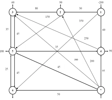
model using an MIP model, Inventory planning, and a delivery route model. These three phases are concerned as an iterative design. Their proposed MIP model is divided into two parts as mentioned in the basic concept. The first is the objective function and the constraints refer to the second part. Its aim is to minimise the total costs consisting of product delivery costs from factories to wholesalers, fixed and variable costs at wholesalers, and product delivery cost from wholesalers to retailers as a description of the objective function. The constraints for this model are the production and throughput capacity, customer demands and material flow requirement. There is a type of constraints specifying the number of products that must be positive and another constraint involves controlling binary variables. It is indicated that using those three steps mentioned above leads to more accurate results and the model can be quickly adapted to market changes. Chopra and Meindl proposed the network optimization models for facility location and capacity allocation using an MIP model to find the best locations for company facilities [16]. Another researchs [17 and 18] involved locating international facilities using a mixed-integer programming model. The main reason for this is that exporting products to foreign markets is difficult due to expensive transportations. Consider a directed and connected network, where the n nodes include at least one supply node and at least one demand node. The decision variables are:
ij
X = flow through arc (i,j); and the given information includes: . i node at generated flow Net Nbi ). j , i ( arc for capacity Arc AUij ). j , i ( arc through flow unit per Cost Costij = = =
The value of bi depend on the nature of node i,
where: node. te intermedia an is i node if , 0 Nbi . node supply a is i node if , 0 Nbi . node demand a is i node if , 0 Nbi = < >
The objective is to minimise the total cost of sending the available supply through the network
to satisfy the given demand. Therefore, the network problem may be written as:
Minimise: ∑ = ∑= = n 1 i n 1 j CostijXij
Z (1)
Subject to: i Nb j ij X k ki
X −∑ =
∑ ; i = 1, 2, ..., n; (2)
AUij Xij
0≤ ≤ ; for each arc (i, j). (3)
The first summation in the node constraints (2) represents the total flow into node
i,
whereas the second summation represents the total flow out of node i. Therefore, the difference is the net flow generated at this node. In some applications, it is necessary to have a lower bound ALij>0 for theflow through each line (i,j) when this occurs, the
translation of variables, Xij/=Xij−ALij is
introduced, with (X ALij) '
ij+ being substituted for
ij
X throughout the model in order to convert the
balance equation for each node in the network. The flow variables Xij have either 0, +1 or -1 coefficients
in these equations. Furthermore, each variable appears in only two balance equations, once with a -1 coefficient, corresponding to the node from which the arc emanates; and once with a +1 coefficient, corresponding to the node upon which the arc is incident. This type of balance equations is referred to as a node-arc incidence matrix; it completely describes the physical layout of the network.
3. LINEAR PROGRAMMING APPLIED TO THE TRANSPORTATION PROBLEM
First, a basic feasible solution must be determined. Although, in the case of the transportation problem, an initial basic feasible solution is easy to
determine by, for example, the Northwest-corner method, the Minimum matrix method, or the Vogel’s approximation method, in the general case an initial basic feasible solution may be difficult to find. The difficulty arises from the fact that the upper and lower bounds on the variables are treated implicitly and, hence, non-basic variables may be at either bound. Basic feasible solutions can be obtained by ‘solving’ spanning trees’-a spanning tree is a connected sub-set of a network including all nodes and containing no loops. A spanning tree solution is obtained as follows:
Step 1. For the arcs not in the spanning tree, set
variables equal to zero;Step 2. For the arcs that are in the spanning tree
(the basic arcs), solve for variables in the system of linear equations provided by the node constraints. To determine whether this initial basic feasible solution is optimal, first the multipliers, yi(i=1,2,...,n) are determined and then checked if these multipliers satisfy:
ij AL ij X ; 0 j y i y ij Cost ij ost
C = − + ≥ = (4)
ij AU ij X ij L A ; 0 j y i y ij Cost ij ost
C = − + = < < (5)
ij AU ij X ; 0 j y i y ij Cost ij ost
C = − + ≤ = (6)
If all the above conditions are met then the solution is an optimal one. A spreadsheet model for solving the car distribution problem is presented. The cells represent the decision variables. These cells indicate the number of cars to be transported between each of the locations. The total cost associated with any transportation plan is computed. A separate constraint is needed for each node in a network flow problem. If supplies are represented by negative numbers and the demands are represented by positive numbers. To solve this problem one should attempt to minimise the total cost by changing the number of cars transported between the various locations while keeping the net number of cars flowing through each location greater than or equal to the supply or demand for cars in each location. Of course, this will also require that the number of cars transported between locations not to be less than zero. The Simplex method of solving this linear program is applied by using the Solver facility within Excel. The values indicate the optimal number of cars that should be transported between each of the locations. The value indicates that the total cost of this transportation plan is 25300 units.
4. GENETIC ALGORITHMS
During the last decade, genetic algorithm-based approaches have received increased attention from the engineers dealing with problems, which could not be solved using conventional problem solving techniques. A typical task of a genetic algorithm in this context is to find the best values of a predefined set of free parameters associated with either a process model or a control vector. A possible solution to a specific problem can be encoded as an individual or a chromosome, which
parents and offspring, once again on the basis of their fitness. A binary chromosome consists of binary digits. A 1 or 0 in the string may, in a Boolean scheme, correspond to whether some condition is true or false, or bits may be strung together to form binary words that will translate either directly or indirectly into continuous valued variables. The first step in the application of a GA is the coding of the variables that describe the problem [20-31]. The most common coding method is to transform the variables to a binary string of specific length. This string represents the chromosome of the problem and the length of the chromosome represents the number of zeros and ones in the binary string. By decoding the individuals of the initial population, the solution for each specific instance is determined and the value of the objective function that corresponds to this individual is evaluated. This applies to all members of the population. Genetic algorithms require the natural parameter set of the optimisation problem to be coded as a finite length string. For the car distribution example, there are 16 decision variables dij as follows:
76 d ,..., 23 d , 14 d , 12
d (7)
A spreadsheet model for solving this problem is presented. The cells represent the chromosome (decision variables) as follows:
11 Q ., . . , 3 Q , 2 Q , 1
Q (8)
These cells correspond to the arcs in reference [19] and indicate the number of cars to be transported between each of the locations. When it comes to reproduction a GA may operate in a generation mode or in a ‘steady-state’ mode. In generation mode iteration of the GA produces a whole new generation of chromosomes. In contrast, the steady-state GA produces, at iteration, just one new ‘child’ chromosome from two selected parents. This child is added to the existing population and the least fit member of the population is then deleted to maintain the population size. The steady-state GA is used in this paper. The advantage of using steady-state reproduction is that all the genes are not lost as is the case in generational replacement where after replacement many of the best individuals may not be produced at all, and their genes may be lost.
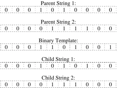
Steady-state reproduction is a better model of what happens in longer-lived species in nature. This allows parents to nurture and teach their offspring, but also gives rise to competition between them. Baker suggested rank selection [21]. Sort the population from best to worst, assign the number of copies that each individual should receive according to a non-increasing assignment function, and then perform proportionate selection according to that assignment [22]. Ranking is a two-step process. First, the list of individuals must be sorted, and next the assignment values must be used in some form of proportionate selection. Some qualitative theory regarding such schemes was presented by Grefenstette [23]. A rank based method is used here. The members are ranked in order of their fitness and the probability of selection is inversely rated to this ranking. The advantage of a rank based approach is that it helps to avoid too rapid a rate of convergence that may lead to the population being swamped by a local optimum due to the loss of diversity. Syswerda [24] proposed uniform crossover which works as follows. Two parents are selected, and two children are produced. For each bit position on the two children, it is decided randomly as to which parent contributes its bit value to which child. Figure 2 shows uniform crossover in action. For each bit position in the parents, a random binary template indicates which parent will contribute its value in that position to the first child. The second child receives the bit value in that position from
Parent String 1:
0 0 0 1 0 1 0 0 0 0
Parent String 2:
0 0 0 0 1 1 1 1 0 0
Binary Template:
0 0 0 1 1 0 1 0 0 1
Child String 1:
0 0 0 1 0 1 0 1 0 0
Child String 2:
0 0 0 0 1 1 1 0 0 0
the other parent.
Uniform crossover generally works better than one and two-point. It was shown by Syswerda that in almost all cases, uniform crossover is more effective at combining schemata than either one or two point crossover. Empirically, uniform crossover is shown to be more effective on a variety of function optimisation problems. In this paper one child is formed by taking a mixture of bits from its two parents according to a random bit string. The proportion of bits coming from the best parent is defined by the user-defined crossover rate in the range zero to one. Where a ‘1’ in the random bit string indicates that in that position the child inherits the corresponding bit from parent-1, whilst a ‘0’ causes inheritance from parent-2. The final step in the implementation of the GA is the application of the fitness function. In this case the objective is the minimisation of the network’s cost function, so the fitness value is the reciprocal of this cost. Before this function is applied, the string must be decoded. Then, once the real value for each parameter is available, the fitness for that specific individual can be estimated. Within the spreadsheet, it shows the total cost of the car distribution problem is 25300 units. One of the advantages of the GA seen here is that the algorithm is only using fitness values for searching and thus solving the problem, in contrast to linear programming which needs a spanning tree to solve the problem and other specific knowledge of the application. The other attractive property of the GA that is demonstrated is its ease of application. Spreadsheets are used widely in industry due to such factors as their versatility, ease of use, rapid development and ease of modification. For over a decade spreadsheets have provided intuitive applications. Bodily [32] stated that the adoption of spreadsheets as decision making aids by end-users was due to the natural interface that exists for model building, the ease of use in terms of inputs, solutions and report generation, and the ability to perform ‘what-if’ analysis. He continued that, because of these key properties, the spreadsheet medium could be used as a stepping stone for bringing operations research models and techniques to the end-user. Recent literature supports Bodily's conclusions, with successful applications in queuing systems, inventory management, aggregate planning, and analysis of manufacturing systems, financial
planning, warehousing and transportation. Techniques and models include linear programming, integer programming, dynamic programming, simulation and heuristics. Spreadsheets are particularly suitable for network planning due to their fundamental representation of data in the form of easily understood tables. The work presented here was carried out using the MicrosoftR ExcelTM spreadsheet and an add-in to provide the GA. This add-in is called EvolverTM and is developed and supplied by Axcelis [33]. The use of this proprietary software demonstrates how simple it is to implement the GA approach to the minimum cost flow problem and transportation problem and also enables the immediate implementation, by any reader, of the methods presented here. This is a key aspect of this paper. The model of network planning developed in this research is built in ExcelTM using the spreadsheet's built-in functions. After building the model, the GA is run to optimise the network given an objective function. The fitness value and decision variables are passed back to the GA component which is independent of the spreadsheet model. At the end of the GA run, when the stopping criterion is met, the best network is presented in a tabular form in the spreadsheet.
5. EMPIRICAL STUDIES
elementary statistical analysis such as [34-36] for a more detailed account. ANOVA procedures utilize a class of continuous probability distributions called F-distributions for the ratio of two variances being tested to see if they are significantly different. Probabilities for a random variable that has an distribution are equal to areas under an F-curve. An F-distribution depends on two numbers of degrees of freedom. The first number of degrees of freedom for an F-curve is called the ‘degrees of freedom for the numerator’ and the second the ‘degrees of freedom for the denominator’. Some basic properties of F-curves are as follows: i. The total area under an curve is equal to 1; ii. An F-curve starts at 0 on the horizontal axis and extends indefinitely to the right; iii. An F-curve is not symmetrical, but is skewed to the right; that is, it climbs to its high point rapidly and comes back to the horizontal axis more slowly. Areas under F-curves have been compiled and put into tables. The table used here is given in reference [34].The optimal solution is found 25300 by genetic algorithm. For this problem, the following GA parameter values were used in analysis of variance experiments to analyse the effects of the parameters on the number of iterations required to reach the optimal fitness. (Population Size: 20,50,80, Crossover Rate: 0.2,0.4,0.5,0.6,0.8, Mutation Rate: 0.001,0.006,0.011,0.016). For each combination of the parameters the GA is run for 8 different random initial populations-these 8 populations being different for each combination. Thus, in total, the GA is run 480 times. The values chosen for the population size are representative of the range of values typically seen in the literature. If the mutation rate is too low, then many genes that would have been useful are never tried out. If it is too high, there will be too much random configuration, offspring will start losing their similarity to their parents, and the algorithm will lose the ability to learn from previous searches. It is normally the case that the mutation rate needs to be small to be effective - as in the range of values used here. The crossover rates chosen are representative of the entire range. The data provide sufficient evidence to conclude that the means for the five different crossover rates are not significantly difference and that the crossover rate is therefore an insignificant factor across the range [0.2:0.8] in the performance of GA. A steady-state
GA has been employed rather than generational replacement. This means that at iteration two parent chromosomes are selected from the population for reproduction. These parents produce a child which is added into the existing population and the weakest member of the population is then deleted. In contrast, a generational GA produces a whole new population of children at iteration. Uniform crossover has been used following the recommendation of Syswerda. The GA has been implemented as an ‘add-in’ to a proprietary spreadsheet in which the network model is constructed. Table 1 shows the natural logarithm of the number of iterations for different mutation rates with the crossover rate fixed at 0.60 and a population size of 50. Table 2 displays the one-way ANOVA table for this data. If the value of the F falls in the rejection region i.e. F > Fcrit, then reject the null hypothesis; otherwise, do not reject the null hypothesis. In Table 2, F = 6.93801160, this falls in the rejection region. Thus the null hypothesis is not accepted. The data provide sufficient evidence to conclude that the means for the four different mutation rates are significantly difference and that the mutation rate is therefore an significant factor across the range [0.001:0.016] in the performance of GA.
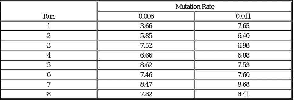
The analysis of variance of mutation rate shows that mutation is a significant factor. This shows that there is clearly little difference in performance in the two mid-values of mutation rate [0.006 and 0.011]. Table 3 shows the natural logarithm of the number of iterations for different mutation rates with the crossover rate fixed at 0.60 and a population size of 50. Table 4 displays the one-way ANOVA table for this data. In Table 4, F =0.9780499, this does not fall in the rejection region. Thus the null hypothesis is accepted. The data provide sufficient evidence to conclude that the means for the two different mutation rates are insignificantly difference and that the mutation rate is therefore an insignificant factor across the range [0.006:0.011] in the performance of GA.
TABLE 1. Natural Logarithm of the Number of Iterations for Different Mutation Rates with Crossover Rate = 0.60 and Population Size = 50.
Mutation Rate
Run 0.001 0.006 0.011 0.016
1 7.33 5.99 7.36 9.1
2 9.23 5.5 6.9 8.2 3 7.7 7.38 6.78 7.8 4 9.3 6.33 6.9 8.45 5 9.23 8.32 7.57 7.65
6 9.17 7.25 7.9 8.44
7 9.95 8.4 8.9 9.2
8 9.07 7.89 8.5 9.23
TABLE 2. One-way ANOVA for Mutation Rate using Results in Table 1.
Groups Count Sum Average Variance
Column 1 8 70.9 8.8725 0.78299285
Column 2 8 57.0 7.1325 1.18285
Column 3 8 60.8 7.60125 0.6144125
Column 4 8 68.0 8.50875 0.3844125
ANOVA
Source of Variation SS df MS F P-value F crit
Between Groups 15.42667 3 5.142225 6.93801160 0.0012323 2.94668526
Within Groups 20.75267 28 0.74116696
Total 36.17935 31
TABLE 3. Natural Logarithm of the Number of Iterations for Different Mutation Rates with Crossover Rate = 0.60 and Population Size = 50.
Mutation Rate
Run 0.006 0.011
1 3.66 7.65
2 5.85 6.40
3 7.52 6.98
4 6.66 6.88
5 8.62 7.53
6 7.46 7.60
7 8.47 8.68
TABLE 4. One-way ANOVA for Mutation Rate using Results in Table 3.
Groups Count Sum Average Variance
Column 1 8 57.06 7.1325 1.18285
Column 2 8 60.81 7.60125 0.6144125
ANOVA
Source of Variation SS df MS F P-value F crit
Between Groups 0.878906 1 0.878906 0.9780499 0.33946 4.6001099
Within Groups 12.58083 14 0.898631
Total 13.45974 15
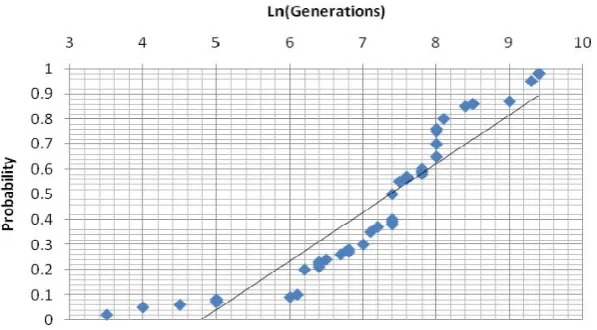
Figure 3. Anderson-darling normality test for number of iterations.
Observation (i), which tells us that the value of the crossover rate is not significant in the broad range [0.2:0.8]. Observation (ii) tells us that the value of the mutation rate is important. As the mutation rate increases so the GA is replaced by a more random search. As mutation tends towards 0 so movements around the search space, and subsequent diversity in the population, is lost due to the comparative rarity in actually applying mutation. Whilst there may be concern that in practical applications a ‘good’ value must be identified for the mutation rate, this concern is reduced by knowing from Observation (iii) that the good values appear to occupy a ‘good range’, rather than being some difficult to isolate single value. Observation (iv) tells us that the effect of the population size does not vary across the range [20,50,80] when using a ‘good’ mutation rate. This changes with the ‘poorer’ mutation rates. This shows that if the mutation rate is too low, then a larger population is required to get the necessary diversity. If the mutation rate is too high, then a smaller population is required. Put the other way round, if the population size is small a higher mutation rate is required to compensate for the reduced potential for diversity across a smaller population, whilst as population size grows, the need for mutation is reduced. Observation (v) tells us that changing crossover rate does not alter the significance of population size for the ‘poorer’ mutation values, i.e. changing crossover rate does not compensate for the ‘poorer’ mutation rate. This result means that methods of statistical analysis based on assumptions of normality may be applied to the log of the number of iterations required by the GA to reach the optimal solution.
6. SIMULATED ANNEALING
The concept is based on the way liquid freezes or metal recrystallizes in the process of annealing. In an annealing process a melt, initially at high temperature and disordered, is slowly cooled so that the system at any time is approximately in thermodynamic equilibrium. As cooling proceeds, the system becomes more ordered and approaches a frozen ground state at zero temperature. Hence, the process can be thought of as an adiabatic
approach to the lowest energy state. If the initial temperature of the system is too low or cooling is done insufficiently slowly the system may become quenched forming defects or freezing out in metastable states i.e., trapped in a local minimum energy state. Like tabu search, simulated annealing allows uphill moves. However, while tabu search in essence makes only uphill moves when it is stuck in local optima, simulated annealing can make uphill moves at any time. It relies heavily on randomization. It is basically a local search algorithm, with the current solution wandering from neighbour to neighbour as the computation proceeds. The key difference from other approaches is that simulated annealing examines neighbours in random order, moving to the first one seen that is either better or else passes a special randomized test. Simulated annealing is an intelligent approach designed to give a good though not necessarily optimal solution, within a reasonable computation time. The motivation for simulated annealing comes from an analogy between the physical annealing of solid materials and optimisation problem. Simulated annealing simulates the cooling process of solid materials-known as annealing. However this analogy is limited to the physical movement of the molecules without involving complex thermodynamic systems.
a solid material so that it reaches a low energy state. Initially the solid is heated up to the melting point. Then it is cooled very slowly allowing. The simulated annealing algorithm was employed to solve this problem. The same 16-bit binary string representation scheme applied in the case of the GA was implemented for simulate annealing because of its flexibility and ease of computation. The cost function for this problem is objective function given in Equation 9.
Minimise: ,
n
1 i
n
1 j
CostijXij
Z ∑
= ∑=
= (9)
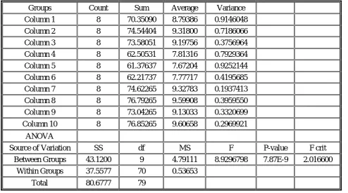
The algorithm was implemented in Turbo C++. The initial stopping criterion was set at a total unit cost of optimal solution found by the genetic algorithm. Ten cooling rates were used (0.40, 0.45, 0.50, 0.60, 0.65, 0.70, 0.80, 0.85, 0.90, 0.95). The final cost function is 25300. Table 5 shows the natural logarithm of the number of iterations for different cooling rates with T = 1500. Table 6 displays the one-way ANOVA table for this data. If the value of the F falls in the rejection region i.e. F > Fcrit, then reject the null hypothesis; otherwise, do not reject the null hypothesis. In Table 6, F = 8.9296798, this falls in the rejection region. Thus the null hypothesis is not accepted. The data provide sufficient evidence to conclude that the means for the ten different cooling rates are significantly difference and that the cooling rate is therefore an significant factor across the range [0.40:0.95] in the performance of simulated annealing.
The analysis of variance of cooling rate shows that cooling is a significant factor. This shows that there is clearly little difference in performance in the three mid-values of cooling rate [0.60;0.65 and 0.70]. Table 7 shows the natural logarithm of the number of iterations for different cooling rates with T = 1500. Table 8 displays the one-way ANOVA table for this data. In Table 8, F = 0.06036, this does not fall in the rejection region. Thus the null hypothesis is accepted. The data provide sufficient evidence to conclude that the means for the three different cooling rates are insignificantly difference and that the cooling rate is therefore an insignificant factor across the range [0.60:0.70] in the performance of simulated annealing.
Therefore the solution found by the GA, SA and linear programming was accepted as the optimal solution the transportation problem. Figure 5 shows the convergence of the total unit cost and iterations when using the simulated annealing with the original set of parameter values to solve the system network.
7. CONCLUSIONS
Genetic algorithms give an excellent trade-off between solution quality and computing time and flexibility for taking into account specific constraints in real situations. The results of the experiment have confirmed that the cooling rate determines the quality of the solutions. If the cooling rate is too low, the configuration can not achieve the optimal solution before it reaches the maximum number of iterations. If the cooling rate is too high, the process could become stuck at a local optimum.
TABLE 5. Natural Logarithm of the Number of Iterations for Different Cooling Rates with T = 1500.
Cooling Rate 0.40 0.45 0.50 0.60 0.65 0.70 0.80 0.85 0.90 0.95
Run 1 7.60 7.82 8.16 8.45 8.47 8.41 8.92 8.92 8.92 8.92
Run 2 9.60 10.11 9.80 7.60 8.10 7.70 9.90 10.10 9.80 8.80
Run 3 10.20 10.20 9.13 7.30 8.70 7.80 9.10 8.80 8.80 9.80
Run 4 8.75 8.45 8.90 6.40 6.10 6.90 8.80 9.87 9.10 10.11
Run 5 9.65 9.87 10.1 8.80 6.90 7.90 9.60 9.7 8.30 10.12
Run 6 8.76 9.78 9.50 8.60 8.30 8.10 9.70 10.2 8.90 9.50
Run 7 7.89 8.97 8.76 6.90 6.70 6.80 8.90 10.3 10.12 9.40
Run 8 7.90 9.34 9.23 8.45 8.10 8.60 9.70 8.9 9.10 10.20
TABLE 6. One-way ANOVA for Cooling Rates using Results in Table 4.
Groups Count Sum Average Variance
Column 1 8 70.35090 8.79386 0.9146048
Column 2 8 74.54404 9.31800 0.7186066
Column 3 8 73.58051 9.19756 0.3756964
Column 4 8 62.50531 7.81316 0.7929364
Column 5 8 61.37637 7.67204 0.9252144
Column 6 8 62.21737 7.77717 0.4195685
Column 7 8 74.62265 9.32783 0.1937413
Column 8 8 76.79265 9.59908 0.3959550
Column 9 8 73.04265 9.13033 0.3320699
Column 10 8 76.85265 9.60658 0.2969921
ANOVA
Source of Variation SS df MS F P-value F crit
Between Groups 43.1200 9 4.79111 8.9296798 7.87E-9 2.016600
Within Groups 37.5577 70 0.53653
Total 80.6777 79
TABLE 7. Natural Logarithm of the Number of Iterations for Different Cooling Rates with T = 1500.
Cooling Rate 0.60 0.65 0.70
Run 1 8.45 8.47 8.41
Run 2 7.60 8.10 7.70
Run 3 7.30 8.70 7.80
Run 4 6.40 6.10 6.90
Run 5 8.80 6.90 7.90
Run 6 8.60 8.30 8.10
Run 7 6.90 6.70 6.80
can do this relatively rapidly and because the mutation operator diverts the method away from local optima, which will tend to become more common as the search space increases in size. Empirical analysis of the performance of GA’s, simulated annealing and the effects of GA’s parameters and simulated annealing on this performance in addition to the aforementioned advantages shows that GA’s and simulated annealing are a feasible, robust and practical engineering tool and are considered further in this paper for minimum cost flow problem programming in response to the weaknesses seen in the mathematical methods that are conventionally applied to network programming. Finally, the analysis of variance of mutation rates and cooling rates has been shown that mutation and cooling are a significant factor.
8. ACKNOWLEDGEMENTS
The work was supported by the University of Yazd (Iran) and Liverpool (U.K.)
9. REFERENCES
1. Munakata, T. and Hashier, D.J., “A Genetic Algorithm Applied to the Maximum flow Problem”, Proceedings of the Fifth International Conference on GA, (1993), 488-493.
2. Winston, W., “Operations Research Applications and Algorithms”, Wads Worth, Inc., Duxbury, Belmont (Calif.), (1994).
3. Ozan, T.M., “Applied Mathematical Programming for Production and Engineering Management”, Prentice-Hall, U.S.A., (1986).
TABLE 8. One-way ANOVA for Cooling Rates using Results in Table 5.
Groups Count Sum Average Variance
Column 1 8 62.5053 7.81316 0.79293
Column 2 8 61.3763 7.67204 0.92521
Column 3 8 62.2173 7.77717 0.41956
ANOVA
Source of Variation SS df MS F P-value F crit
Between Groups 0.08603 2 0.04301 0.06036 0.94158 3.466800112
Within Groups 14.9640 21 0.71257
Total 15.0500 23
4. Wang, G., Wan, Z., Wang, X. and Lv, Y., “Genetic Algorithm Based on Simplex Method for Solving Linear-Quadratic Bilevel Programming Problem”, Computers and Mathematics with Applications, Vol. 56, No. 10, (2008), 2550-2555.
5. Grosan, C., Abraham, A. and Ishibuchi, H., “Hybrid Evolutionary Algorithms, Studies in Computational Intelligence”, Springer-Verlag Berlin Heidelberg, N.Y., U.S.A., (2007).
6. Haupt, R.L. and Haupt, S.E., “Practical Genetic Algorithms”, Second Edition, John Wiley and Sons, Inc., Hoboken, New Jersey, U.S.A., (2004).
7. Zak, J., “Multiple Criteria Evaluation and Optimization of Transportation Systems”, Journal of Advanced Transportation, Vol. 43, No. 2, (2009), 91-94.
8. Tao, Y., “Improved Genetic Algorithm for Fixed Charge Transportation Problem”, International Symposium on Computational Intelligence and Design, (2008). 9. Lin, C.H., “Genetic Algorithm for Shortest Driving Time
in Intelligent Transportation Systems”, International Conference on Multimedia and Ubiquitous Engineering, (2008).
10. Sadegheih, A., “Scheduling Problem Using Genetic Algorithm, Simulated Annealing and the Effects of Parameter Values on GA Performance, Applied Mathematical Modelling, Vol. 30, No. 2, (2006), 147-154.
11. Sadegheih, A., “Evolutionary Algorithms and Simulated Annealing in the Topological Configuration of the Spanning Tree”, WSEAS Transactions on Systems, Vol. 7, No. 3, (2008), 114-124.
12. Xu, T., Wei, H. and Hu, G., “Study on Continuous Network Design Problem using Simulated Annealing and Genetic Algorithm”, Expert Systems with Applications, Vol. 36, No. 2, (2009), 1322-1328.
13. Lau, H.C.W., “Benchmarking of Optimisation Techniques Based on Genetic Algorithms, Tabu Search and Simulated Annealing”, International Journal of Computer Applications in Technology, Vol. 28, No. 2, (2007), 209-219.
14. Silva, C.A., Runkler, T.A., Sousa, J.M. and Palm, R., “Ant Colonies as Logistic Processes Optimizers”, Third International Workshop, ANTS, Brussels, Belgium, (2002). 15. Ma, H. and Suo, C., “A Model for Designing Multiple Products Logistics Networks”, International Journal of Physical Distribution and Logistics Management, Vol. 36, No. 2, (2006), 127-135.
16. Chopra, S. and Meindl, P., “Supply Chain Management Strategy, Planning and Operations”, 3rd ed., Pearson Education, Inc., New Jersey, (2007).
17. Canel, C. and Khumawala, B.M., “A Mixed-Integer Programming Approach for the International Facilities Location Problem”, International Journal of Operations and Production Management, Vol. 16, No. 4, (1996), 49-68.
18. Ostermark, R., “Invited Paper: A Flexible Platform for Mixed-Integer Non-Linear Programming Problems”, Kybernetes, Vol. 36, No. 6, (2007), 652-670.
19. Sadegheih, A. and Drake, P.R., “Network Optimization Using Linear Programming and Genetic Algorithm”, Neural Network World, Int. J. on Non-Standard
Comput. and AI, Vol. 3, (2001), 223-233.
20. Davis, L., “Handbook of Genetic Algorithms”, Reinhold, New York, U.S.A., (1991).
21. Baker, J.E., “Adaptive Selection Methods for GA’s”, in J.J.Grefenstette,ed., Proceedings of First International Conference on GA’s, Erlbaum, (1985), 101-111. 22. Goldberg, D.E. and Deb, K., “A Comparative Analysis
of Selection Schemes Used in GA’s”, In G. Rawlins, ed., Foundations of GA’s, Morgan Kaufmann, (1991). 23. Grefenstette, J.J. and Baker, J.E., “How GA’s Work: A
Critical Look at Implicit Parallelism”, Proceedings of Third International Conference on GA’s, (1989), 20-27. 24. Syswerda, G., “Uniform Crossover in Genetic
Algorithms”, In J. David Schaffer ed., Proceedings of the third International Conference on Genetic Algorithms, San Mateo, Calif Morgan Kaufmann Publishers, (1989), 2-9.
25. Juang, Y.S., Lin, S.S. and Kao, H.P., “An Adaptive Scheduling System with Genetic Algorithms for Arranging Employee Training Programs”, Expert System with Applications, Vol. 33, (2007), 642-651.
26. Canyurt, O.E. and Ozturk, H.K., “Three Different Application of Genetic Algorithm Search Techniques on Oil Demand Estimation”, Energy Conversion and Management, Vol. 47, (2006), 3138-3148.
27. Kaya, I. and Engin, O., “A New Approach to Define Sample Size at Attributes Control Chart in Multistage Processes: An Application in Engine Piston Manufacturing Process”, Journal of Material Processing Technology,Vol. 183, (2007), 38-48.
28. Tavakkoli-Moghaddam, R., Sayarshadand, H.R. and ElMekkawy, T.Y., “Solving a New Multi-Period Mathematical Model of the Rail-Car Fleet Size and Car Utilization by Simulated Annealing”, International Journal of Engineering, Transactions A: Basics, Vol. 22, No. 1, (2009), 33-46.
29. Tavakkoli-Moghaddam, R. and Mehdizadeh, E., “A New LIP Model for Identical Parallel-Machine Scheduling with Family Setup Times Minimizing the Total Weighted Flow Time by a Genetic Algorithm”, International Journal of Engineering, Transactions A: Basics, Vol. 20, No. 2, (2007), 183-194.
30. Tavakkoli-Moghaddam, R., Jolai, F., Khodadadeghan, Y. and Haghnevis, M., “A Mathematical Model of a Multi-Criteria Parallel Machine Scheduling Problem: A Genetic Algorithm”, International Journal of Engineering, Transactions A: Basics, Vol. 19, No. 1, (2006), 79-86.
31. Porto, V.W., Saravanan, N., Waagen, D. and Eiben, A. E., “Evolutionary Programming VII”, 7th International Conference, San Diego, California, U.S.A., (1998), 735-744.
32. Bodily, S.E., “Spreadsheet Modelling as a Stepping Stone”, Interfaces, Vol. 16, No. 5, (1986), 34-52. 33. “Evolver User’s Guide”, Axcelis, Inc., Seattle, W.A.,
U.S.A., (1995).
34. Weiss, N. A., “Elementary Statistics”, Second Edition, Addison-Wesley Publishing Company, Inc., San Francisco, London, U.K., (1993).
and Sons, Inc., New York, U.S.A., (1994).
36. Ryan, B.F. and Joiner, B.L., “Minitab Handbook”, Third Edition, Includes Releases 7-9, Wads Worth, Inc., Duxbury, Belmont (Calif.), (1994).
37. Kirkpatrick, A.S., Gelatt, C.D. and Vecchi, M.P., “Optimization by Simulated Annealing”, Science, Vol. 220, No. 4598, (1983), 671-680.
38. Sohrabi, B. and Bassiri, M.H., “Experiments to Determine the Simulated Annealing Parameters Case
Study in VRP”, International Journal of Engineering, Transactions B: Applications, Vol. 17, No. 1, (2004), 71-80.
39. Azencott, R., “Simulated Annealing Parallelization Techniques, John Wiley and Sons, Inc., N.Y., U.S.A., (1992).