Comparing time series transcriptome data between plants using a network module finding algorithm

METHODOLOGY

Comparing time series transcriptome data

between plants using a network module finding

algorithm

Jiyoung Lee

_{, Lenwood S. Heath}

_{, Ruth Grene}

_{and Song Li}

Abstract

Background: Comparative transcriptome analysis is the comparison of expression patterns between homologous genes in different species. Since most molecular mechanistic studies in plants have been performed in model species, including Arabidopsis and rice, comparative transcriptome analysis is particularly important for functional annota-tion of genes in diverse plant species. Many biological processes, such as embryo development, are highly conserved between different plant species. The challenge is to establish one-to-one mapping of the developmental stages between two species.

Results: In this manuscript, we solve this problem by converting the gene expression patterns into co-expression networks and then apply network module finding algorithms to the cross-species co-expression network. We describe how such analyses are carried out using bash scripts for preliminary data processing followed by using the R programming language for module finding with a simulated annealing method. We also provide instructions on how to visualize the resulting co-expression networks across species.

Conclusions: We provide a comprehensive pipeline from installing software and downloading raw transcriptome data to predicting homologous genes and finding orthologous co-expression networks. From the example provided, we demonstrate the application of our method to reveal functional conservation and divergence of genes in two plant species.

Keywords: Comparative transcriptome analysis, Network, Sequence homology, Arabidopsis, Soybean, Embryo development

© The Author(s) 2019. This article is distributed under the terms of the Creative Commons Attribution 4.0 International License (http://creat iveco mmons .org/licen ses/by/4.0/), which permits unrestricted use, distribution, and reproduction in any medium, provided you give appropriate credit to the original author(s) and the source, provide a link to the Creative Commons license, and indicate if changes were made. The Creative Commons Public Domain Dedication waiver (http://creat iveco mmons .org/ publi cdoma in/zero/1.0/) applies to the data made available in this article, unless otherwise stated.

Background

Expression analysis is commonly used to understand the tissue or stress specificity of genes in large gene fami-lies [1–5]. The goal of comparative transcriptome analy-sis is to identify conserved co-expressed genes in two or more species [3, 6, 7]. The traditional definition of orthologous genes is based solely on sequence homology [8–11] and syntenic relationships [2, 12–14] and not at all on gene expression patterns. In contrast, compara-tive transcriptome analysis combines a comparison of gene sequences with a comparison of expression patterns

between homologous genes in different species. Homol-ogous genes have been reported to be expressed at dif-ferent developmental stages, in difdif-ferent tissue types, or under different stress conditions [3, 15–17]. This docu-mented divergence of expression patterns provides cru-cial evidence for the existence of functional divergence of homologous genes across species [18, 19]. Therefore, comparative transcriptome analysis is an important tool for distinguishing those genes that have retained func-tional conservation from those that have undergone functional divergence. Comparative transcriptome anal-ysis is particularly important for plant research, since most molecular mechanistic studies in plants have been performed in model species, primarily Arabidopsis thali-ana [20]. The consequence of this narrow focus is that

Open Access

*Correspondence: [email protected]

1 _{Genetics, Bioinformatics and Computational Biology, Virginia}

the functional annotation of the genes of many other plant species relies solely on sequence comparisons with Arabidopsis [21].

To compare transcriptomes between any two spe-cies, a first step is to establish homologous relationships between proteins in the two species. A second step is to identify expression data obtained from experiments that are performed under similar conditions or tissue types. The third step is to compare the expression patterns between the two data sets. In this protocol, we will com-pare published time course seed embryo expression data from Arabidopsis [22] with data from the same tissue in soybean [23] as a demonstration of how to apply compu-tational tools to comparative transcriptome analysis.

In contrast with the time course data examined here, many other data sets have been reported from “treat-ment–control” experiments (one time point only and two treatment conditions). For example, soybean roots were treated with drought stress in one experiment [4]. To address the question of functional conservation ver-sus functional divergence within gene families, these soy-bean root data can be compared with transcriptome data from Arabidopsis roots, under a similar stress [24]. This is a relatively simple problem, because, in both experi-ments, we can identify lists of differentially expressed genes in response to the same or similar treatments. It is a simple two-step process to identify conserved co-expressed genes for treatment–control experiments. First, one needs to identify a list of gene pairs that are homologous between these two species. A simple BLAST search or other more sophisticated approaches, such as OMA, EggNog, or Plaza [9, 10, 12], can be used to iden-tify homologous genes. Second, the two lists of differen-tially expressed genes can be compared to find whether any pairs of these homologous genes appear in both lists.

In this article, we are focusing on a more complex sce-nario: two time-series experiments were performed for the same developmental process in two different spe-cies [25]. Time course data provide more data points than simple treatment–control experiments and, thus, can reveal relationships based on development between homologous genes in two organisms. However, this is also challenging, because the number of time points in the two experiments are different. It can be challenging to precisely match developmental stages between two species, although some excellent approaches have been proposed [25, 26]. Despite the difficulty of establish-ing a one-to-one mappestablish-ing between the developmental stages of two species, many biological processes, such as embryo development, are known to be highly conserved between different plant species that are compared in comparative transcriptome analysis [27, 28]. One way to solve this developmental stage problem is to convert the

gene expression patterns into a co-expression network and then apply network alignment or network module finding algorithms to these co-expression networks [29]. Transforming expression data to a network form simpli-fies the problem and allows exploration using well estab-lished network algorithms [30, 31]. Here, we describe how to perform such analysis using a published simulated annealing method [29]. We also discuss how to visualize the resulting co-expression networks across species [32] and the results from different choices of homology find-ing methods.

Results

Comparative transcriptome analysis overview

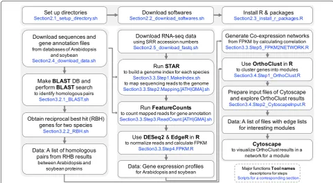
This protocol provides details of comparative transcrip-tome analysis between two species. We not only compute sequence similarity between protein coding genes in two species, we also integrate the gene expression patterns of these genes from two different species under similar biological processes. There are three major steps in this analysis (Fig. 1): (1) identify homologous genes between two species; (2) generate a gene expression data matrix and a co-expression network in each species; (3) perform cross species comparisons of gene homology and expres-sion patterns. For each of these steps, multiple bioinfor-matics tools are available. This protocol will provide a basic workflow for each of the steps and the reader can substitute individual steps with other tools (see “ Discus-sion” section). To facilitate reproducible and effective computational analysis [33, 34], we suggest that the user creates a folder structure (Fig. 2) such that the raw data, processed data, results, and scripts for data processing can be organized into their respective folders.

Obtaining reciprocal best hit (RBH) genes

Reciprocal best BLAST hit (RBH) is a commonly used method to identify homologous genes in two species [35–41]. To identify RBH genes between any two spe-cies, the BLAST results from protein sequence alignment were first parsed to identify the best BLAST hit for each soybean protein in the Arabidopsis protein list. For each soybean protein, there was at most one best BLAST hit protein in the Arabidopsis proteome. For each of the Arabidopsis proteins identified in the first step, the best BLAST hit of each protein in the soybean proteome was also identified. If this best hit was also the original homologous gene found in the first step, this pair of pro-teins was defined to constitute an RBH pair.

two species from BLAST results. The user can download this script from a GitHub repository for this pipeline (https ://githu b.com/LiLab AtVT/Compa reTra nscri ptome .git). Although RBH genes are widely used in comparative genomic analysis, other methods can be used to identify homologous genes for downstream analysis (see “ Discus-sion” section). An example file (ARATH2GLYMA.RBH. subset.txt) of RBH genes is provided. The user can use this file to perform the following analysis without run-ning the RBH script. The summary statistics for the RBH analysis results are provided in Table 1. We found 13,024 RBH pairs in these two species and these genes pairs were used in this analysis.

Co‑expression networks

Co-expression network generation was followed by gene expression data processing steps using the same pipeline for both species. For this step, we used 1267 Arabidop-sis genes and 2092 soybean genes that are known to be essential for embryo development in Arabidopsis [27, 42] and soybean [23]. To convert the gene expression profiles into gene co-expression networks, we first filtered genes with low expression levels and low variation across con-ditions from the gene expression profiles. After that, we calculated gene co-expression matrices using the Pearson Correlation Coefficient (PCC). PCC and the p-values of

PCC were used to filter genes (see “Methods” section). From a total of 24,148 Arabidopsis genes, 1267 genes were selected for the co-expression network analysis. After filtering by PCC and p-values, 1092 genes remained and were used to construct a co-expression matrix. A total of 595,686 co-expression edges were initially gen-erated from the PCC step; 17,648 co-expression edges among 853 genes remained after filtering. For the soy-bean co-expression network, 62,185 co-expression edges among 1401 genes were finally obtained.

OrthoClust analysis

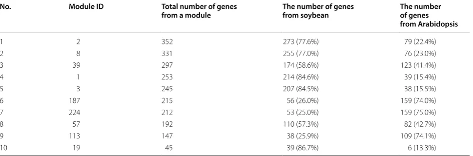
From the previous steps, we generated two co-expression networks and a list of homologous pairs for the selected genes of these two species as inputs to the OrthoClust analysis. The examples of three input data files are provided in Table 2. OrthoClust integrated gene co-expression networks of Arabidopsis and soybean with orthologous pairs of the genes from two species and clus-tered three kinds of relations into cross-species modules. From one trial of the OrthoClust analysis, we obtained 353 modules and ranked them according to the total number of genes from a module as an example (Table 3). Some modules contain genes from both species with some level of balance, and other modules have one spe-cies only.

Fig. 1 A workflow of comparative transcriptome analysis between soybean and Arabidopsis. It is composed of three major parts: identification of

Visualization of OrthoClust results as a network

To visualize OrthoClust results, we used Cytoscape, a network visualization platform to analyze biological net-works and to integrate multiple data into netnet-works such as gene expression profiles or annotation [43]. We used module 8 from the previous step as an example. There are three input files: (1) the soybean co-expression network edge list for genes in module 8, (2) the Arabidopsis co-expression network edge list for genes in module 8, and (3) the RBH list for genes in module 8.

As an example of the network with module 8, nodes and edges from soybean and Arabidopsis genes were

Files generated during the processes Files from github repository

Files to be downloaded by the user PRJNAtest.txt

PRJNA197379.txt PRJNA301162.txt Protein sequences

Reference genome/ gene annotation [ATH|GMA]_STAR-2.5.2b_index BLAST

sratoolkit.2.8.2-1-centos_linux64 bin fastq-dump STAR-2.5.2b bin Linux_x86_64_static STAR subread-1.5.1-Linux-x86_64 bin featureCounts OrthoClust_1.0.tar.gz

R Libraries: DESeq2/EdgeR/OrthoClust Cytoscape

Section2.1_setup_directory.sh Section2.2_download_softwares.sh Section2.3_install_r_packages.R Section2.4_download_data.sh Section2.5_download_fastq.sh Section3.2.1_BLAST.sh Section3.2.2_RBH.sh Section3.3.Step1.MakeIndex.sh Section3.3.Step2.Mapping.ATH.sh Section3.3.Step2.Mapping.GMA.sh Section3.3.Step3.ReadCount.ATH.sh Section3.3.Step3.ReadCount.GMA.sh Section3.3.Step4.FPKM.R

Section3.3.Step5_FPKM2NETWORK.R Section3.4.Step1_OrthoClust.R Section3.4.Step2_CytoscapeInput.R

ARATH2GLYMA.RBH.subset.txt bam

rc

fpkm ATH PRJNA301162.csv

GMA PRJNA197379.csv OrthoClustResults.csv

ExpressionProfile_Module8.pdf

Cytoscape_Input-edge_[ATH|GMX|RBH].csv SRR830182.log

SRR830182.err

Fig. 2 Folder structure for data analysis

Table 1 Results of Identified Orthologous Genes

Species Soybean Arabidopsis

Number of proteins

(Total number of gene models) 48,375(56,044) 24,148(37,336) Blast results in each species

(Query: Blast DB) 1,086,080(Soybean: Arabi-dopsis)

1,081,623

(Arabidopsis: Soybean)

Number of RBH genes in each

species 13,024 13,024

Number of 5 best hit in each

indicated by green and orange colors respectively. To highlight genes of interest, we used thicker double lines for edges and blue color for nodes. We separated genes into four groups according to their input files and species and laid out each of them with a Degree Sorted Circle Layout (Fig. 3).

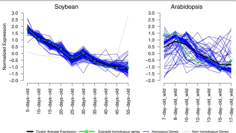
Visualization of OrthoClust results as expression profiles To understand expression patterns of genes from the selected modules under different stages of embryo development, we visualized gene expression profiles for module 8 (Fig. 4). In this module, most soybean genes are tightly clustered. Some Arabidopsis genes are tightly clustered (close to the black line) whereas other Arabidopsis genes are not. This result shows that many genes in the soybean co-expression cluster change their expression patterns in Arabidopsis, sug-gesting potential functional divergence of these genes. In contrast, many genes that are RBH pairs in the two species have similar expression patterns. For example, one gene (AT5G52560, green line) that is related to the raffinose biosynthetic pathway has a similar decreasing

expression pattern as its RBH gene (Glyma.04G245100) in soybean.

Effect of different parameters in OrthoClust analysis

We analyzed how different parameters affect the results of this analysis. We focus on two parameters (Fig. 5), the Pearson Correlation Coefficient (PCC) threshold that was used to convert co-expression data to networks and the coupling constant κ (kappa) that was used in OrthoClust analysis. We found that using a higher PCC threshold resulted in higher number of modules, which is expected because higher threshold in PCC resulted in fewer co-expression edges and smaller modules in the network. We found that using κ = 1 resulted in more modules as compared to using κ = 0. This is because that when κ = 0, the edges that represent homologous genes between two species are not used in the clustering analysis (see “ Dis-cussion” section). The parameter κ represents the relative weights of co-expression edges and homology edges in the module finding algorithm. We found that the number of modules does not increase dramatically when we set κ = 2 or 3 (see “Discussion” section for the effect of changing κ). Table 2 Examples of input data files for OrthoClust analysis

There are three inputs: two co-expression networks of (A) soybean and (B) Arabidopsis, (C) orthologous pairs between soybean and Arabidopsis.

(A) (B) (C)

Row Column Row Column Soybean gene Arabidopsis gene

Glyma.01G006400 Glyma.01G016500 AT1G01540 AT1G05350 Glyma.01G001300 AT2G07050 Glyma.01G021300 Glyma.01G021400 AT1G06040 AT1G06150 Glyma.01G005800 AT4G29310 Glyma.01G019400 Glyma.01G022500 AT1G01720 AT1G07400 Glyma.01G006100 AT4G26300 Glyma.01G015400 Glyma.01G026700 AT1G05230 AT1G07570 Glyma.01G010100 AT1G32090 Glyma.01G025100 Glyma.01G026700 AT1G02660 AT1G08230 Glyma.01G015400 AT2G35470 Glyma.01G025100 Glyma.01G028900 AT1G01090 AT1G08510 Glyma.01G019400 AT5G65670

Table 3 Top 10 OrthoClust results sorted by the total number of genes from a module

OrthoClust was performed with parameters κ = 3, gene co-expression correlation cutoff ≥ 0.99 and homologous pairs obtained from RBH Blast No. Module ID Total number of genes

from a module The number of genes from soybean The number of genes from Arabidopsis

1 2 352 273 (77.6%) 79 (22.4%)

2 8 331 255 (77.0%) 76 (23.0%)

3 39 297 174 (58.6%) 123 (41.4%)

4 1 253 214 (84.6%) 39 (15.4%)

5 3 245 207 (84.5%) 38 (15.5%)

6 187 215 56 (26.0%) 159 (74.0%)

7 224 212 53 (25.0%) 159 (75.0%)

8 57 192 110 (57.3%) 82 (42.7%)

9 113 147 38 (25.9%) 109 (74.1%)

Discussion

This protocol organized a number of computational tools into a pipeline to perform comparative transcrip-tome analyses. Depending on the species of interest, their available databases, or user preferences, there are multiple alternative bioinformatics tools for each step. For example, in searching for homologous genes, several other substitutable tools, such as OMA or OrthoFinder [10, 11], can be used instead of BLAST. A comprehensive comparison of these tools is out of the scope of this manuscript. Some databases or tools provide pre-computed homologous genes [8, 12]. Addi-tional steps must be performed to ensure that the gene ids from OMA [10], OrthoFinder [11], or PLAZA [12] match the gene ids used in the expression analysis.

Moreover, in terms of clustering methods, we adapted OrthoClust, which provides a framework for module finding based on searching a lowest energy level of its cost function using simulated annealing. This approach can be expanded to other inputs such as by using many-to-many homologous relations in two species and by inferring modules across more than two species. There are other novel comparative transcriptome approaches that can be applicable to inter- or intra-species analysis (Table 4). For example, a modified K-mean clustering method was used for co-clustering transcriptome data from maize and rice after different segments of devel-oping leaves [44]. In this work, a unified developmental model (UDM) was established by an iterative algorithm using approximately 3000 selected anchor genes which

Glyma.13G166200 Glyma.05G229300 Glyma.09G194900 Glyma.19G082800 Glyma.03G199500 Glyma.03G086100 Glyma.07G009100 Glyma.02G084100 Glyma.03G186200 Glyma.14G005100 Glyma.07G041000 Glyma.06G150100 Glyma.04G025400 Glyma.02G259800 Glyma.15G132200 Glyma.19G204400 Glyma.08G335700 Glyma.19G226400 Glyma.06G170800 Glyma.09G026100 Glyma.02G279300 Glyma.13G049700 Glyma.08G292700 Glyma.11G015600 Glyma.13G372300 Glyma.15G176500 Glyma.08G207300 Glyma.07G130400 Glyma.20G176900 Glyma.20G110400 Glyma.16G100200 Glyma.19G075100 Glyma.08G146500 Glyma.02G005700 Glyma.04G034000 Glyma.12G226400 Glyma.01G144900 Glyma.03G179800 Glyma.16G053200 Glyma.02G256800 Glyma.12G038200 Glyma.14G205600 Glyma.08G058600 Glyma.01G035600 Glyma.08G036400 Glyma.09G020100 Glyma.04G168300 Glyma.13G241100 Glyma.13G206500 Glyma.02G203900 Glyma.17G051400 Glyma.02G186100 Glyma.10G172200Glyma.13G301300 Glyma.14G170900Glyma.19G147400 Glyma.06G127200 AT4G35590 AT3G66658 Glyma.07G247100 Glyma.15G110200 AT5G54390 AT5G14950 Glyma.13G157800 AT3G60860 AT2G40820 AT2G26080 AT4G38520 AT3G03450 AT3G30841 AT1G01060 AT5G40760 AT1G11910 Glyma.17G033100 Glyma.12G148400 Glyma.17G047000 Glyma.19G260900 Glyma.15G015700 Glyma.13G100600 Glyma.16G009700 Glyma.06G166200 Glyma.09G171600 Glyma.09G200300 Glyma.12G076200 Glyma.06G320700 Glyma.08G252700 Glyma.08G227000 Glyma.05G230700 Glyma.14G021800 Glyma.08G217500 Glyma.04G215900 Glyma.12G092200 Glyma.15G170900 Glyma.02G272400 Glyma.01G057100 AT1G60800 AT3G58690 AT2G41820 AT3G16110 AT3G49590 AT3G15940 AT2G39805 AT5G28300 AT3G15430 AT2G26580 Glyma.19G053500 Glyma.01G117800 Glyma.01G170200 Glyma.09G129500 Glyma.03G156600 Glyma.17G130200 Glyma.04G245100 Glyma.08G125400 Glyma.04G202900 Glyma.13G279000 Glyma.02G094400 Glyma.17G027200 Glyma.06G077700 Glyma.10G139200 Glyma.05G151100 Glyma.18G132000 Glyma.14G068700 Glyma.02G218100 Glyma.16G158200 Glyma.12G140100 Glyma.13G120000 Glyma.18G282000 Glyma.15G003600 Glyma.08G011600 Glyma.07G024100 Glyma.15G150100 Glyma.11G120900 Glyma.08G187500 Glyma.06G130700 Glyma.01G164500 Glyma.18G058800 Glyma.10G095500 Glyma.13G327500 Glyma.16G177400 Glyma.08G274200 Glyma.01G021400 AT3G47500 AT1G22060 AT4G36360 AT5G01310AT1G48175 AT4G22130 AT3G55470 AT1G03080 AT5G52560 AT5G41960 AT5G13660 Glyma.14G187000 Glyma.07G102900 Glyma.18G221200 Glyma.19G140100 Glyma.03G124300 Glyma.11G085500 Glyma.01G230300 Glyma.14G065500 Glyma.20G106800 Glyma.13G068100 Glyma.07G084900 Glyma.09G011200 Glyma.09G007200 Glyma.18G040000 Glyma.02G308100 Glyma.19G143000 Glyma.10G153200 Glyma.02G290700 Glyma.04G199300 Glyma.06G015400 Glyma.20G109400 Glyma.09G131800 Glyma.15G038100 Glyma.17G072000 Glyma.18G034300 Glyma.02G229900 AT4G38040 AT4G18030 AT5G54160 AT3G24630 AT5G50860 AT5G40610 AT1G72480 AT3G07680 Glyma.06G137100 Glyma.07G105400 Glyma.08G212900 Glyma.18G279400 Glyma.02G247900 Glyma.14G195400 Glyma.10G069600 Glyma.09G044300 Glyma.11G251700 Glyma.19G251000 Glyma.07G049100 Glyma.15G001200 Glyma.19G131400 Glyma.15G197800 Glyma.04G013900 Glyma.09G013900 Glyma.10G161200 Glyma.05G207100 Glyma.13G278300 Glyma.02G295100 Glyma.10G282900 Glyma.18G116800 Glyma.08G082500 Glyma.04G125500 Glyma.05G048200 Glyma.15G073300 Glyma.15G177600 Glyma.03G125200 Glyma.11G055200 Glyma.17G128300 Glyma.11G179000 Glyma.12G038900 Glyma.12G227300 Glyma.10G212900 Glyma.09G214500 Glyma.13G241000 Glyma.06G074400 Glyma.09G251300 Glyma.19G165200 Glyma.10G163400 Glyma.09G172700 Glyma.06G094300 Glyma.11G226400 Glyma.11G115000 Glyma.04G066900 Glyma.01G001300 Glyma.19G105900 Glyma.04G147100 Glyma.18G070800 Glyma.03G191700 Glyma.11G062900 Glyma.01G227200 Glyma.14G083500 Glyma.17G010600 Glyma.12G020700 Glyma.12G089000 Glyma.20G019700Glyma.18G224200 Glyma.12G211000 Glyma.15G140000 Glyma.05G110200 Glyma.20G005900 Glyma.02G275300 Glyma.16G049300 Glyma.18G017200 Glyma.03G252000 Glyma.20G022900 Glyma.14G035400 Glyma.02G033400 AT4G30260 AT5G42020 AT5G45290 AT3G44340 AT4G23850 AT1G14010 AT3G14870 AT4G33580 AT1G10700 AT1G32090 AT4G28050 AT5G19930 AT3G58640 AT2G27810 AT5G42620 AT1G16780 AT4G01210 AT1G23190 AT1G53050 AT1G01540 Glyma.02G266900 Glyma.08G002700 Glyma.06G289300 Glyma.06G106900 Glyma.15G168700 Glyma.05G026200 Glyma.13G289900 Glyma.17G228800 Glyma.15G013400 Glyma.05G070000 Glyma.13G083400 Glyma.05G025900 Glyma.04G107100 Glyma.02G036500 Glyma.19G136100 Glyma.01G021300 Glyma.08G257600 Glyma.20G224000 Glyma.16G063200 Glyma.07G256500 Glyma.06G227200 Glyma.20G189900 Glyma.17G154400 Glyma.19G222700 Glyma.19G209500 Glyma.07G177100 Glyma.06G150000 Glyma.02G101500 AT5G47530 AT3G15850 AT4G15840 AT4G14240 AT3G13510 AT5G24060 AT3G17810 AT1G05350 AT1G74960 AT1G21980 AT3G17940 AT2G41540 AT5G13300 AT5G61790 Glyma.12G220400 Glyma.12G174200 Glyma.06G265800 Glyma.06G169700 Glyma.17G098200 Glyma.13G192400 Glyma.11G112000 Glyma.03G140700 Glyma.17G201000 Glyma.13G274800 Glyma.17G226100 Glyma.12G107600 Glyma.13G107400 Glyma.04G173100 Arabidopsis Genes Soybean Genes Arabidopsis Coexpression Edges Soybean Coexpression Edges Homology Edges Circle 1

Circle 2 Circle 3

Circle 4

Fig. 3 Visualization of module 8 from OrthoClust result. In this network, Circle 1 and 4 stand for groups of genes from Arabidopsis and soybeans

are homologous genes with similar expression pat-terns in two species. As compared to this method, our approach is more flexible because our approach does not require construction of UDM. Another example is the breadth-first search algorithm (TO-GCN) for time-ordered co-expression networks of transcription fac-tors in maize [45]. In this work, maize and rice gene expressions used to construct co-expression networks separately, and maize specific TF-gene pairs were selected for experimental validation. In comparison to this work, we are using homologous information as

edges in our network construction whereas TO-GCN focused on TF-target co-expression edges but did not include homologous relationships in their networks.

Many genes in both species were not included in the RBH gene lists. This is because the criterion for iden-tifying RBH genes is highly stringent. It requires that both genes in two species be the best BLAST hit in their respective species. This can be relaxed to identify k-best-hits in two species [6]. We have developed a script that can generate k-best-hits using BLAST results between any two species: OrthologousGenes_OneWayTopNBes-tHit.py, which is available in the github repository of this project.

The parameter κ is used to adjust the relative impor-tance of the co-expression edges and homologous edges in network module finding algorithms (Fig. 5). When κ equals zero, the module finding method only finds co-expression modules and does not consider the effects of homologous edges. When κ is set to be higher than zero, homologous edges will be included in the module find-ing objective function. This can be verified by comparfind-ing the numbers of modules found when κ = 0 to numbers of modules found when κ > 0. The numbers of modules found when κ = 1 is two to three times the numbers of modules found when κ = 0. This result suggests that including homologous edges generates more modules

Nor

maliz

ed Expression

−2.0 −1.5 −1.0 −0.5 0.0 0.5 1.0 1.5 2.0 2.5 3.0

5−da

ys−old

10−da

ys−old

15−d

ay

s−old

20−da

ys−old

25−da

ys−old

30−d

ay

s−old

35−d

ay

s−old

40−d

ay

s−old

45−da

ys−old

55−da

ys−old

−2.0 −1.5 −1.0 −0.5 0.0 0.5 1.0 1.5 2.0 2.5 3.0

7−da

y−old_wild

8−da

y−old_wild

10−da

y−old_wild

12−da

y−old_wild

13−da

y−old_wild

15−da

y−old_wild

17−da

y−old_wild

Cluster Average Expression Example homologous genes Homogous Genes Non−homologous Genes

Soybean

Arabidopsis

Fig. 4 Expression plots of genes from Arabidopsis and soybean bellowing to one of modules of OrthoClust result. One example of homologous

genes in Arabidopsis and soybeans are AT5G52560 and Glyma.04G245100 are highlighted in green

Fig. 5 Effect of different correlation cutoff and κ values on the

across species, because, when κ = 0, all modules are from

the same species. Comparing the numbers of modules from κ = 2 with κ = 1 and κ = 3 with κ = 2 suggest that

increasing κ can further increase the number of modules. The PCC threshold also affects the number of modules identified (Fig. 5). For the same κ value, a higher PCC threshold always leads to more modules. This is expected as a co-expression network with higher PCC threshold contains fewer edges. Because of the reduced number of edges, the network is less connected and can be break into more modules as compared to the network gener-ated with lower PCC threshold.

Conclusions

In this article, we have presented a method to perform comparative transcriptome analysis. We provided a flex-ible workflow in publicly accessflex-ible scripts with detailed annotations. A users can use simple commands to exe-cute the scripts following the instructions provided in the method section. From the sample analysis, we showed how orthologous relations in two species can be identi-fied by reciprocal best hits (RBHs), what kinds of filtering methods can be applied to co-expression profiles, how to run the clustering methods, and how to visualize the results. Using this pipeline, we identified a module that includes genes that play important roles in embryo devel-opment in both species. We further explored this module by visualizing the inferred relationships of genes in the module as a network and by comparing expression pat-terns of the genes to understand conserved gene function between the two species. Using our proposed method, we were able to observe the conserved expression pat-tern and the example homologous genes in the example module from both species. In conclusion, our proposed method can be used to identify homologous genes with correlated expression patterns in two species.

Methods

Install software and download experimental data

All scripts used in this analysis can be obtained from github using the following command. (the git software is installed in most Linux systems by default. If git is not installed in your system, please refer to https ://git-scm. com for installation instructions).

$ git clone https ://githu b.com/LiLab AtVT/Compa reTra nscri ptome .git ATH_GMA

All code blocks started with “$” are command line scripts that should be executed under a Linux terminal. All code blocks started with “>” are command line scripts that should be executed under an interactive R program-ming language console.

You can replace “ATH_GMA” with another folder name that better represents your project. All scripts in this pro-ject are tested under the propro-ject folder created by the “git clone” command (default ATH_GMA).

Necessary resources

This protocol was tested under CentOS 7, which is a Linux-based operating system distribution. The steps described in this protocol can be used in most UNIX-like operating systems; this includes all major Linux distribu-tions, and Mac OSX. For Windows users, the individual components of this protocol, such as BLAST, software used for RNA-Seq analysis, and programming languages R and Python, all have Windows-compatible executable files and can be used under Windows environments. In this protocol, we will install NCBI BLAST for the homol-ogy search step, STAR for read mapping and feature Counts for counting reads, and the R programming lan-guage and several packages for RNA-Seq and compara-tive transcriptome analysis.

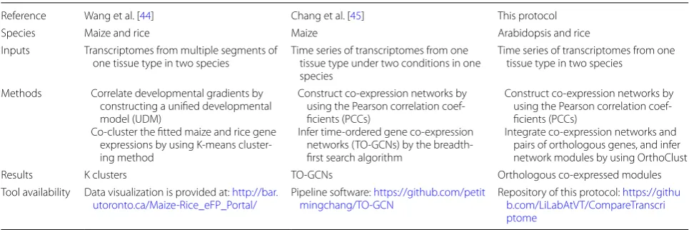
Table 4 Comparison of published methods that compare co-expression patterns across different plant species

Reference Wang et al. [44] Chang et al. [45] This protocol

Species Maize and rice Maize Arabidopsis and rice

Inputs Transcriptomes from multiple segments of

one tissue type in two species Time series of transcriptomes from one tissue type under two conditions in one species

Time series of transcriptomes from one tissue type in two species

Methods Correlate developmental gradients by constructing a unified developmental model (UDM)

Co-cluster the fitted maize and rice gene expressions by using K-means cluster-ing method

Construct co-expression networks by using the Pearson correlation coef-ficients (PCCs)

Infer time-ordered gene co-expression networks (TO-GCNs) by the breadth-first search algorithm

Construct co-expression networks by using the Pearson correlation coef-ficients (PCCs)

Integrate co-expression networks and pairs of orthologous genes, and infer network modules by using OrthoClust

Results K clusters TO-GCNs Orthologous co-expressed modules

Tool availability Data visualization is provided at: http://bar.

Set up a folder structure for data analysis

In this protocol, the reader can use the following com-mands to create the recommended folder structure (Fig. 2).

$ cd ATH_GMA

$ mkdir raw_data processed_data scripts results software

$ mkdir processed_data/bam processed_data/rc

Sequence and annotation files from databases should be downloaded to the raw_data folder. Software tools that will be used in this analysis can be saved and installed in the software folder. We recommend that the reader creates a folder named bin under the software

folder such that the executable files can be copied to soft-ware/bin folder and add software/bin to the PATH envi-ronmental variable under the Linux environment. For experienced Linux users, software can also be installed in a user specified folder such as ~/bin or in a system wide folder. The reader can download scripts in github into the scripts folder. Intermediate output will be generated in the processed_data folder, and major input and output files for visualization will be saved in the results folder.

All scripts for this step are provided in Section2.1_setup_ directory.sh in the scripts folder. The reader can set up the folder structure (Fig. 2) using the following command.

$ cd ATH_GMA

$ sh ./scripts/Section2.1_setup_directory.sh

Software installation

We provide a script to download and install tools for RNA-seq analysis; readers can run the script in the pro-ject folder.

$ cd ATH_GMA

$ sh ./scripts/Section2.2_download_software.sh

A successfully installed tool will return version infor-mation when it is run with a -v or a --version option.

Install NCBI BLAST for identification of homologous genes BLAST is a sequence similarity search tool [46]. The lat-est version of NCBI BLAST can be downloaded from the NCBI ftp site using the following link: ftp://ftp.ncbi.nlm. nih.gov/blast/executables/LATEST/. This folder con-tains precompiled executable files and installation files for Windows, Mac OSX, and Linux platforms. Because finding orthologous genes at a genome scale is compu-tationally intensive, it is recommended to use a Linux workstation or computing cluster to perform the BLAST analysis.

For Linux users, the current pre-compiled execut-able is ncbi-blast-2.6.0 + -x64-linux.tar.gz.

For Mac users, the current installation file is ncbi-blast-2.6.0 + .dmg.

For Windows users, the current installation file is ncbi-blast-2.6.0 + -win64.exe.

A later version of BLAST should work as well with minor changes in the command line options. For Win-dows and Mac users, double click the downloaded file to install the program. For Linux users, one can use

$ tar –xvf ncbi-blast-2.6.0+-x64-linux.tar.gz

to extract the archive file. After extracting the files, move the executable files to a folder in the Linux search path.

Install tools for RNA‑Seq data download

The following shows a sample script to download sra-tools and fastq-dump to download the raw sequencing data. The sequence read archive (SRA) database provides sra-toolkit, which is a suite of easy to use computational tools to download data from the database. To download the raw data from the SRA database, one needs to first install the sra-toolkit and use the fastq-dump utility pro-gram based on the SRA ids.

$ cd ATH_GMA/software

$ wget http://ftp-trace.ncbi.nlm.nih.gov/sra/sdk/cur-rent/sratoolkit.current-centos_linux64.tar.gz $ tar -xzf sratoolkit.current-centos_linux64.tar.gz $ ./sratoolkit.2.8.2-1-centos_linux64/bin/fastq-dump --version

Install tools for RNA‑Seq data analysis

We will install the STAR [47] and featureCounts [48] software tools. STAR is a read mapper, and feature-Counts can count the number of reads mapped to each gene in the genome. Both software tools were used here due to their speed and accuracy [49, 50]. Other alterna-tive mappers can be used, and there are excellent review papers [50–52] that compare and summarize these differ-ent bioinformatics tools.

To download and install STAR and featureCounts, run the following scripts in the project folder.

$ cd Proj_CompTS_ATH_GMA/software

$ wget https ://githu b.com/alexd obin/STAR/archi ve/2.5.2b.tar.gz

$ tar -xzf 2.5.2b.tar.gz

$ tar -zxvf download

$ subread-1.5.1-Linux-x86_64/bin/featureCounts -v

Install R and DESeq2 packages for RNA‑Seq data analysis

R is a programing language and environment for sta-tistical data analysis [53]. We will use R to summarize RNA-Seq reads and to generate FPKM data. To install R, the reader should go to the Comprehensive R Archive Network (CRAN) (https ://cran.r-proje ct.org) to download the installer packages for their Windows, Mac OSX, or Linux system. For Linux users, R can be installed using the command line, and platform dependent package management systems. For exam-ple, to install R in CentOS 7 Linux, the user should simply type:

$ sudo yum install R

Scripts for installing R packages are provided in:

Section2.3_install_r_packages.R

This R script can be run on a Linux or MAC terminal by executing the script with the Rscript command directly, or a shell script that is a wrapper of the R script we provide.

$ cd ATH_GMA

$ Rscript ./scripts/Section2.3_install_r_packages.R or

$ sh ./scripts/Section2.3_install_r_packages.sh

To install DESeq2  [54], the user should follow the instruction for the respective package. This package is part of the Bioconductor repository such that the installation should be performed using the Biocon-ductor installation script. The following commands are executed under the R environment and these com-mands are preceded by “>”. For comcom-mands that are executed under Linux terminals, these commands are preceded by “$”.

> source(‘https ://bioco nduct or.org/biocL ite.R’) > biocLite(‘DESeq2’)

The installation script will detect the dependency of these two packages and install other required packages accordingly.

To install the OrthoClust package, the user should download the script for the OrthoClust package.

> setwd(“./software”)

> install.packages(“OrthoClust_1.0.tar.gz”, repos = NULL, type = “source”)

Download protein and genome sequences for Arabidopsis and soybean

Sample scripts for download are provided in “Section2.4_ download_data.sh”. All protein-coding sequences and genomic sequences for Arabidopsis can be downloaded from the Araport web site (www.arapo rt.org). Araport is a data portal for Arabidopsis genomic research that hosts the latest genomic sequences and genome annota-tions for this model organism [55]. The web site requires free registration to access the download link to the pro-tein sequences and genome annotation files. As of July 2017, the current version of the protein sequences file is “Araport11_genes.201606.pep.fasta.gz”. This name will likely be different for future versions of the protein sequences. We recommend that users download the latest version of the protein sequences, and record the actual download date and version of the sequence files for the purpose of reproducibility. The latest version of the genome sequence of Arabidopsis is “TAIR10_Chr. all.fasta.gz”. This file is unlikely to change because the genome assembly of Arabidopsis is likely to remain the same in the future. The latest version of the gene annota-tion file is “Araport11_GFF3_genes_transposons.201606. gtf.gz”.

All protein-coding sequences for soybeans can be downloaded from the DOE phytozome database (https :// phyto zome.jgi.doe.gov/pz/porta l.html#!bulk?org=Org_ Gmax). Phytozome is a data portal for plant and micro-bial genomes that hosts dozens of sequenced plant genomes and gene annotations [56]. This web site also requires free registration before data downloading. The latest version of soybean protein sequences is version 2.0 (downloaded in July 2017). The protein sequences and genomic sequences are “Gmax_275_Wm82.a2.v1.protein. fa.gz” and “Gmax_275_v2.0.fa.gz”. These names are likely to change with future versions of the genome and pro-teome annotation. The latest version of the gene annota-tion file is “Gmax_275_Wm82.a2.v1.gene_exons.gff3.gz”.

These files are in compressed fasta format and require decompression before use. Under the Linux command line, the following command can be used to decom-press these *.gz files.

$ gunzip Araport11_genes.201606.pep.fasta.gz $ gunzip Gmax_275_Wm82.a2.v1.protein.fa.gz

Download raw data from published RNA‑Seq experiments

(PRJNA301162 for Arabidopsis [22] and PRJNA197379 for soybean [57]). For the Arabidopsis samples, RNA-Seq data were collected in triplicates at seven time points (7, 8, 10, 12, 13, 15, and 17 days after pollination). For the soybean samples, RNA-Seq data were collected in tripli-cates at ten time points (5, 10, 15, 20, 25, 30, 35, 40, 45, and 55 days, day 0 of the time course is 12 to 17 days after anthesis). Each sample is represented by a unique GSM id; for example, the three replicates of 7 days old Arabi-dopsis embryo samples are GSM1930276, GSM1930277, and GSM1930278. All 41 samples from this experiment are stored under a unique GSE id, GSE74692. Each sam-ple is also represented by a unique SRA id. For examsam-ple, the three replicates of 7  days old Arabidopsis embryo samples are SRR2927328, SRR2927329, and SRR2927330 from PRJNA301162.

$ fastq-dump --split-3 SRR2927328 --outdir ./raw_ data

We suggest that the reader download the data into the raw data folder for further processing. To download large numbers of data sets, prepare a text file with all SRR ids for one species and run the following script in the project folder.

$ cd ATH_GMA

$ sh ./scripts/Section2.5_download_fastq.sh ./raw_ data/PRJNA301162.txt ATH

$ sh ./scripts/Section2.5_download_fastq.sh ./raw_ data/PRJNA197379.txt GMA

Depending on the size of sequencing data and network speed, this step may take a few hours. We provide a test file PRJNAtest.txt for the user to test the execution time for downloading one file. The time for downloading the entire data set can be estimated based on download-ing this sdownload-ingle file. We also provide the FPKM data for this particular data set so that the users do not need to download the original data to perform the analysis in this protocol. To perform the analysis using provided FPKM file, the user can start the analysis from a subsection of methods, Identify orthologous co-expressed clusters using OrthoClust.

Identifying homologous genes between species

Identification of homologous pairs using BLAST

Analysis in this section can be performed using the fol-lowing command:

$ cd ATH_GMA

$ sh ./scripts/Section3.2.1_BLAST.sh

Step 1. Merge the Arabidopsis protein fasta file and

soybean protein fasta file using this Linux command:

$ cat Araport11.pep.fasta GLYMA2.pep.fasta> ATHGMA.pep.fasta

Step 2. Create the BLAST database:

$ makeblastdb -in ATHGMA.pep.fasta \

-out ATHGMA.blastdb \ -dbtype prot \

-logfile makeblastdb.log

The option –in specifies the input file name of the merged protein fasta file. The option –out specifies the BLAST database file name. The option –dbtype indi-cates the database is a protein database. The option –logfile is for recording error messages in case the pro-cess fails.

Step 3. Perform the BLAST search. The Linux command used in this step is:

$ blastp -evalue 0.00001 \

-outfmt 6 -db ATHGMAX.blastdb \

-query ATHGMA.fasta>ATHGMA.pep.blastout

The option -evalue specifies the E value threshold. The option -outfmt is set to be 6, which is tab delimited for-mat. The option -db is set to be the BLAST database built in step 3. The option -query uses the merged protein fasta files as input. The results of BLAST analysis are written in a file named ATHGMA.pep.blastout.

The output includes the following 12 tab-separated columns “qseqid sseqid pident length mismatch gapo-pen qstart qend sstart send evalue bitscore”. The mean-ing of these columns can be found usmean-ing the BLAST help manual. The columns that will be used in downstream analysis are qseqid (query sequence id), sseqid (subject sequence id), and evalue (E value). We will filter BLAST results and only keep homologous genes with BLAST E value < 1e−5 [3, 26].

Obtaining reciprocal best hit (RBH) genes

We developed a Python script that can identify RBH genes from the above two species from BLAST results. The user can download this script from the github repos-itory. To perform the analysis the user can use the follow-ing commands:

$ cd ATH_GMA

Gene expression data processing

Gene expression quantification includes three main steps: 1) read mapping; 2) read counting and 3) FPKM calculation. For this analysis, we follow a published pro-tocol for expression processing [58].

Step 1. Create genome index by STAR

RNA-Seq reads have to be mapped to the respective reference genomes. To use STAR to map reads to the ref-erence genome, the user needs to build a genome index using the following commands.

$ cd ATH_GMA

$ sh ./scripts/Section3.3.Step1.MakeIndex.sh

The following commands are used to create a genome index for Arabidopsis.

$ WORKDIR = $(pwd)

$ IDX = $WORKDIR/raw_data/ATH_STAR-2.5.2b_

index

$ GNM = $WORKDIR/raw_data/TAIR10_Chr.all.

fasta

$ GTF = $WORKDIR/raw_data/Araport11_GFF3_

genes_transposons.201606.gtf

$ STAR --runMode genomeGenerate \

--genomeDir $IDX \ --genomeFastaFiles $GNM \ --sjdbGTFfile $GTF

The option --runMode indicates that the command is to create a genomic index. The option --genomeDir specifies the file name for the genome index. The option --genomeFastaFiles indicates the input fasta file for genomic sequences. The option --sjdbGTFfile is to pro-vide a genome annotation file when creating the genomic index. A genome index will be created for each species.

Step 2. Read mapping by STAR

After creating genome indexes, the user needs to use STAR to map reads from each sample to the reference genome to generate a read mapping file using the follow-ing commands.

$ cd ATH_GMA

$ sh ./scripts/Section3.3.Step2.Mapping.ATH.sh $ sh ./scripts/Section3.3.Step2.Mapping.GMA.sh

The Section3.3.Step2.Mapping.ATH.sh shell script is to map all Arabidopsis reads. The Section3.3.Step2.Map-ping.GMA.sh shell script is to map all Soybean reads. In the SRA database, each sample has a unique SRR id. The following commands show one example of such SRR ids (SRR2927328). SRR2927328_1 and SRR2927328_2 repre-sent two ends of paired reads.

$ STAR --genomeDir $IDX \

--readFilesIn $WORKDIR/raw_data/SRR2927328_1. fastq.gz $WORKDIR/raw_data/SRR2927328_2.fastq.gz \ --outFileNamePrefix $WORKDIR/processed_data/ bam/SRR2927328/SRR2927328 \

--outSAMtype BAM SortedByCoordinate

The option --genomeDir specifies the file name for the genome index. The option --readFilesIn indicates the input fastq files for RNA-seq reads. Two files are provided for paired-end reads. The option --outFile-NamePrefix is to provide the directory for output data. The option --outSAMtype BAM indicate the output file should be a BAM file. SortedByCoordinate sets the out-put data to be sorted by the order of where the read is mapped to the chromosome.

Step 3. Read counting with featureCounts

To count reads with featureCounts, the user can use the following command:

$ cd ATH_GMA

$ sh ./scripts/Section3.3.Step3.ReadCount.ATH.sh $ sh ./scripts/Section3.3.Step3.ReadCount.GMA.sh

For this step, featureCounts will calculate how many reads map to each gene region. For simplicity, we only count uniquely mapped reads and only summarize read counts at the gene level. Other software can be used to summarize expression at isoforms levels. The following commands are for counting reads for a single file.

$ WORKDIR = $(pwd)

$ GTF = $WORKDIR/raw_data/Araport11_GFF3_

genes_transposons.201606.gtf

$ BAM = $WORKDIR/processed_data/bam

$ RC = $WORKDIR/processed_data/rc

$ featureCounts -t exon \

-g gene_id \ -p \ -a $GTF \

-o $RC/SRR2927328.readcount.txt \

$BAM/SRR2927328/SRR2927328Aligned.sortedBy-Coord.out.bam

The option -t exon indicates that only reads mapped to exons are counted. The option -p indicates the input reads are paired-end reads. The option -a provides the location of the genome annotation file. The option -o specifies the output file location. The last parameter is the file name of the read mapping file (BAM file).

Step 4. FPKM calculation using DESeq2

counts from different files into one single file; (2) differen-tial expression analysis using DESeq2; (3) FPKM calcula-tion; and (4) average FPKM calculation across replicates. These steps can be performed using a unified R script: Section3.3.Step4.FPKM.R. To run this script, the user needs to provide a table that summarizes the replicate structure of the samples. Example tables (PRJNA301162. csv for Arabidopsis and PRJNA197379.csv for soybean) are provided in the processed_data folder.

To run the unified R script for FPKM calculation, use the following commands:

$ cd ATH_GMA

$ Rscript ./scripts/Section3.3.Step4.FPKM.R ./pro-cessed_data/fpkm/GMA

$ Rscript ./scripts/Section3.3.Step4.FPKM.R ./pro-cessed_data/fpkm/ATH

This script requires multiple input files to be present in the working directory. These files include a file that describes the design matrix of the experiment and the read count files generated in Step 3. More descriptions of the input file formats are included in the annotation of the R script.

Step 5. Co-expression networks from gene expression

profiles

Expression data will be summarized and converted to gene co-expression networks. The input data include data matrices with averaged and normalized FPKM values. In this protocol, we use genes in metabolic pathways of seed development [28, 42]. Other methods can be used to filter genes before the analysis, for example, only keep genes with high variations across conditions (variance > 0.5) or genes with minimum gene expression level (FPKM ≥ 0.5 from any conditions). Finally, gene co-expression matri-ces were calculated using the Pearson Correlation Coef-ficient (PCC) of the FPKM values between the filtered sample genes for each species. The gene co-expression matrices were converted into co-expression networks with an edge list by treating each gene as a node and a PCC values as an edge between genes after the cut-off with p value < 0.001 and Pearson correlation coefficient > 0.99. To generate co-expression networks from gene expression profiles, the following commands were used.

$ cd ATH_GMA

$ Rscript ./scripts/Section3.3.Step5_ FPKM2NETWORK.R

Identify orthologous co‑expressed clusters using OrthoClust

Overview of the OrthoClust method

Simple approaches can be used to identify conserved co-expression genes across different species. For example,

one can first cluster gene expression in two species sepa-rately, and, for each pair of cluster combinations, one can find whether the pairs of clusters share significantly large numbers of homologous genes using appropriate statistical tests such as Fisher’s exact test. OrthoClust [29] is a global approach in which the process of co-expression clustering finding and homology detection is integrated into the same objective function. The objective function H is defined as

where SN is the sets of genes for a species and a subscript

of S (N = 1 or 2) corresponds to the species respectively. The variables i and j are individual genes of a species or nodes on a network. ΛN

ij denotes a modularity score from

gene i and j, that is a difference between the real number of edges and the expected number of edges. δσ_iσ_j is for a

module label. If genes i and j have the same module label,

δσ_iσ_j= 1, and, if not, δσ_iσ_j= 0. A coupling constant, κ

(kappa) controls overall impact of orthology relations on the objective function, and a weight, w_ij′ is for orthology relations coming from the number of orthologous genes between two species. The objective function H will return lower values when orthologous genes are assigned into the same module.

This approach translates orthologous co-expression finding into a network module finding problem. The objective function includes three components: two com-ponents represent the goodness of the expression cluster-ing results and one component represents the effect of homologous genes across species. The parameter κ can be adjusted to increase or decrease the contribution of homologous genes in the clustering processes.

Steps for OrthoClust analysis

To perform OthoClust analysis, we require three input data files (Table 2): (1) the gene co-expression network from soybean; (2) the gene co-expression network from Arabidopsis; and (3) the orthologous gene pairs between two species.

These files require a specific format for the OrthoClust engine to analyze. The user can use the following R com-mand to perform the clustering analysis:

> library(OrthoClust)

> OrthoClust2(Eg1 = GMX_edgelist, Eg2 = ATH_ edgelist, \

list_orthologs = GA_orthologs, kappa = 3)

We provide a wrapper script that will read three input files: a list of edges from Arabidopsis, a list of edges from

H= −



 �

i,j∈S1

Λ1_ijδσiσj+

�

i,j∈S2

Λ2_ijδσiσj+κ

�

(i,j′ )∈O(S1,S2)

w_ij′δσiσ_j′



soybean, and a list of RBH gene pairs from two species. To perform OrthoClust analysis, the user can simple use the following commands:

$ cd ATH_GMA

$ Rscript ./scripts/Section3.4.Step1_OrthoClust.R

This script will generate three files. Orthoclust_Results. csv contains information regarding modules assignment for each gene. Orthoclust_Results_Summary.csv includes number of genes assigned to each module. Orthoclust_ Results.RData contains multiple R objects that will be used in the visualization step.

Visualization of OrthoClust results as a network

To generate these files for Cytoscape visualization, the user can use the following command.

$ cd ATH_GMA

$ Rscript ./scripts/Section3.4.Step2_CytoscapeInput.R Step 1. To Import three files on Network Browser, we can first start from the Cytoscape menu bar and follow these choices: File > Import > Network > File. After you select one of three input files, the popup window with “Import Network From Table” title appears. You can see two columns with gene names in the middle of the win-dow. Next, to change attributes of columns, click the first line of each column and choose either Source Node or Target Node from the menu. Since three edge lists do not have direction, the two columns from each input file can be assigned into either source or target nodes. After that, we change an option for column names from Advanced Options at the bottom left of the window. On the new popup window, we can uncheck “Use first line as col-umn names”, since we do not have headers in the input files. Finally, you can see two column names, Column1 and Column2 with different icons of attributes, and the remaining parts of the preview are gene names. You can repeat these steps for each of the input files.

Step 2. With three imported networks, we can integrate data sets of co-expression networks with homologous relations using the Union function. To do that, select three networks on the network tab on the control panel (click one network and click the other two networks while pressing Command), and move to Cytoscape’s menu bar: Tools > Merge > Networks.

In the popup window for Advanced Network Merge, we should choose the Union button, select three net-works from Available Netnet-works, and then click the right-facing arrow acting for Add Selected. After that you can find that three networks are now on Networks to Merge, and you can click the Merge button to merge three networks.

The name of the merged network will appear with the total number of merged nodes and edges on the Network tab on the control, and usually it is automatically visual-ized on the Cytoscape canvas.

Step 3. To express properties of networks (species

information, source of edges such as co-expression net-works or homologous relations), we can customize vis-ual attributes of the merged network. To do that, on the Select tab on the control panel, we can click the + icon below Default filter and choose Column Filter to add the new condition. From the Choose column drop-down list, you can select Node: name or Edge: name and type a prefix of each species (“AT” for Arabidopsis genes, or “Glyma” for soybean genes). This filter applies to visuali-zation of the merged automatically, so you can see high-lighted nodes on the Cytoscape canvas.

There are several ways to change visualization proper-ties of the selected components. First, we can set Bypass Style for the selected nodes or edges such as Fill Color and Size for properties of nodes, or Stroke Color and Line Type for properties of edges. To do this, move your mouse pointer on one of the highlighted nodes, right-click, and then select Edit > Bypass Style > Set Bypass to Selected Nodes on the popup menu. The control panel on the left side will be automatically changed to the Style tab, and you can see three subtabs: Node, Edge, and Net-work on the bottom of the interface. Second, we can apply different Layouts with these selected nodes or all nodes from Cytoscape menu bar Layout.

Visualization of OrthoClust results as expression profiles We also provide a R scripts to directly visualize gene expression patterns for orthologous co-expression mod-ules into a figure. This script will generate gene expres-sion profile plots of genes in a selected module including homologous genes of these genes along different time points. It can also highlight expression pattern of inter-esting genes with different color line. The figure can be generated by the following commands:

$ cd ATH_GMA

$ Rscript ./scripts/Section3.4.Step2_CytoscapeInput.R

Acknowledgements

This work is partly supported by Virginia Soybean Board.

Authors’ contributions

JL and SL designed the analysis. RG provided the original data and interpreted the biological results. LH edited the manuscript and provided suggestions to improve the methods. JL developed the methods. SL and JL wrote the manu-script. All authors read and approved the final manumanu-script.

Availability of data and materials

Ethics approval and consent to participate

Not applicable.

Consent for publication

Not applicable.

Competing interests

The authors declare no competing interests.

Author details

1 _{Genetics, Bioinformatics and Computational Biology, Virginia Polytechnic}

Institute and State University, Blacksburg, VA 24061, USA. 2 _Department

of Computer Science, Virginia Polytechnic Institute and State University, Blacksburg, VA 24061, USA. 3 _{School of Plant and Environmental Sciences,}

Virginia Polytechnic Institute and State University, Blacksburg, VA 24061, USA.

Received: 13 November 2018 Accepted: 17 May 2019

References

1. Movahedi S, Van Bel M, Heyndrickx KS, Vandepoele K. Comparative co-expression analysis in plant biology. Plant, Cell Environ. 2012;35:1787–98. 2. Van Bel M, Proost S, Wischnitzki E, Movahedi S, Scheerlinck C, Van de Peer

Y, et al. Dissecting plant genomes with the PLAZA comparative genomics platform. Plant Physiol. 2012;158:590–600.

3. Movahedi S, Van de Peer Y, Vandepoele K. Comparative network analysis reveals that tissue specificity and gene function are important factors influencing the mode of expression evolution in arabidopsis and rice. Plant Physiol. 2011;156:1316–30.

4. Prince SJ, Joshi T, Mutava RN, Syed N, Joao Vitor MS, Patil G, et al. Com-parative analysis of the drought-responsive transcriptome in soybean lines contrasting for canopy wilting. Plant Sci. 2015;240:65–78. 5. Ware D, Jaiswal P, Ni J, Pan X, Chang K, Clark K, et al. Gramene: a resource

for comparative grass genomics. Nucleic Acids Res. 2002;30:103–5. 6. Mutwil M, Klie S, Tohge T, Giorgi FM, Wilkins O, Campbell MM, et al. PlaNet:

combined sequence and expression comparisons across plant networks derived from seven species. Plant Cell. 2011;23:895–910.

7. Ruprecht C, Mendrinna A, Tohge T, Sampathkumar A, Klie S, Fernie AR, et al. FamNet: a framework to identify multiplied modules driving path-way diversification in plants. Plant Physiol. 2016;170:1878.

8. Li LL, Stoeckert CJ, Roos DS. OrthoMCL: identification of ortholog groups for eukaryotic genomes. Genome Res. 2003;13:2178–89.

9. Jensen LJ, Julien P, Kuhn M, von Mering C, Muller J, Doerks T, et al. Egg-NOG: automated construction and annotation of orthologous groups of genes. Nucleic Acids Res. 2007;36:D250–4.

10. Altenhoff AM, Kunca N, Glover N, Train C-M, Sueki A, Piliota I, et al. The OMA orthology database in 2015: function predictions, better plant support, synteny view and other improvements. Nucleic Acids Res. 2015;43:D240–9.

11. Emms DM, Kelly S. OrthoFinder: solving fundamental biases in whole genome comparisons dramatically improves orthogroup inference accuracy. Genome Biol. 2015;16:157.

12. Proost S, Van Bel M, Vaneechoutte D, Van de Peer Y, Inzé D, Mueller-Roeber B, Vandepoele K. PLAZA 3.0: an access point for plant comparative genomics. Nucleic Acids Res. 2014;43:974–81.

13. Proost S, Fostier J, De Witte D, Dhoedt B, Demeester P, Van de Peer Y, et al. i-ADHoRe 30—fast and sensitive detection of genomic homology in extremely large data sets. Nucleic Acids Res. 2012;40:11.

14. Lyons E, Pedersen B, Kane J, Alam M, Ming R, Tang H, et al. Find-ing and comparFind-ing syntenic regions among arabidopsis and the outgroups papaya, poplar, and grape: CoGe with rosids. Plant Physiol. 2008;148:1772–81.

15. Berri S, Abbruscato P, Faivre-Rampant O, Brasileiro ACM, Fumasoni I, Satoh K, et al. Characterization of WRKY co-regulatory networks in rice and arabidopsis. BMC Plant Biol. 2009;9:1–22.

16. Wang Y, Feng L, Zhu Y, Li Y, Yan H, Xiang Y. Comparative genomic analy-sis of the WRKY III gene family in populus, grape, arabidopanaly-sis and rice. Biol Direct. 2015;10:48.

17. Yao X, Ma H, Wang J, Zhang D. Genome-wide comparative analysis and expression pattern of TCP gene families in Arabidopsis thaliana and

Oryza sativa. J Integr Plant Biol. 2007;49:885–97.

18. Netotea S, Sundell D, Street NR, Hvidsten TR. ComPlEx: conservation and divergence of co-expression networks in A. thaliana, Populus and

O. sativa. BMC Genom. 2014;15:106.

19. Roulin A, Auer PL, Libault M, Schlueter J, Farmer A, May G, et al. The fate of duplicated genes in a polyploid plant genome. Plant J. 2013;73:143–53.

20. Provart NJ, Alonso J, Assmann SM, Bergmann D, Brady SM, Brkljacic J, et al. 50 years of Arabidopsis research: highlights and future directions. New Phytol. 2016;209:921–44.

21. Horan K, Jang C, Bailey-Serres J, Mittler R, Shelton C, Harper JF, et al. Annotating genes of known and unknown function by large-scale coexpression analysis. Plant Physiol. 2008;147:41–57.

22. Schneider A, Aghamirzaie D, Elmarakeby H, Poudel AN, Koo AJ, Heath LS, et al. Potential targets of VIVIPAROUS1/ABI3-LIKE1 (VAL1) repression in developing Arabidopsis thaliana embryos. Plant J. 2016;85:305–19. 23. Aghamirzaie D, Nabiyouni M, Fang Y, Klumas C, Heath L, Grene R,

et al. Changes in RNA splicing in developing soybean (Glycine max) embryos. Biology (Basel). 2013;2:1311–37.

24. Kilian J, Whitehead D, Horak J, Wanke D, Weinl S, Batistic O, et al. The AtGenExpress global stress expression data set: protocols, evalua-tion and model data analysis of UV-B light, drought and cold stress responses. Plant J. 2007;50:347–63.

25. Wang L, Czedik-Eysenberg A, Mertz RA, Si Y, Tohge T, Nunes-Nesi A, et al. Comparative analyses of C4 and C3 photosynthesis in developing

leaves of maize and rice. Nat Biotechnol. 2014;32:1158–65.

26. Patel RV, Nahal HK, Breit R, Provart NJ. BAR expressolog identification: expression profile similarity ranking of homologous genes in plant spe-cies. Plant J. 2012;71:1038–50.

27. Junker A, Hartmann A, Schreiber F, Bäumlein H. An engineer’s view on regulation of seed development. Trends Plant Sci. 2010;15:303–7. 28. Chaudhury AM, Koltunow A, Payne T, Luo M, Tucker MR, Dennis ES,

et al. Control of early seed development. Annu Rev Cell Dev Biol. 2001;17:677–99.

29. Yan K-K, Wang D, Rozowsky J, Zheng H, Cheng C, Gerstein M. Ortho-Clust: an orthology-based network framework for clustering data across multiple species. Genome Biol. 2014;15:R100.

30. Palla G, et al. Directed network modules. New J Phys. 2007;9:186. 31. Malliaros FD, Vazirgiannis M. Clustering and community detection in

directed networks: a survey. Phys Rep. 2013;533:86.

32. Smoot ME, Ono K, Ruscheinski J, Wang P-L, Ideker T. Cytoscape 28: new features for data integration and network visualization. Bioinformatics. 2011;27:431–2.

33. Sandve GK, Nekrutenko A, Taylor J, Hovig E. Ten simple rules for repro-ducible computational research. Bourne PE, editor. PLoS Comput Biol. 2013;9:e1003285.

34. Osborne JM, Bernabeu MO, Bruna M, Calderhead B, Cooper J, Dalchau N, et al. Ten simple rules for effective computational research. Bourne PE, editor. PLoS Comput Biol. 2014;10:e1003506.

35. Ward N, Moreno-Hagelsieb G. Quickly finding orthologs as reciprocal best hits with BLAT, LAST, and UBLAST: how much do we miss? de Crécy-Lagard V, editor. PLoS ONE. 2014;9:e101850.

36. Fulton DL, Li YY, Laird MR, Horsman BGS, Roche FM, Brinkman FSL. Improving the specificity of high-throughput ortholog prediction. BMC Bioinformatics. 2006;7:270.

37. Dessimoz C, Boeckmann B, Roth ACJ, Gonnet GH. Detecting non-orthol-ogy in the COGs database and other approaches grouping orthologs using genome-specific best hits. Nucleic Acids Res. 2006;34:3309–16. 38. Tatusov RL, Fedorova ND, Jackson JD, Jacobs AR, Kiryutin B, Koonin EV,

et al. The COG database: an updated version includes eukaryotes. BMC Bioinformatics. 2003;4:41.

39. O’Brien KP, Remm M, Sonnhammer ELL. Inparanoid: a comprehensive database of eukaryotic orthologs. Nucleic Acids Res. 2005;33:D476–80. 40. Jin J, Tian F, Yang D-C, Meng Y-Q, Kong L, Luo J, et al. PlantTFDB 4.0:

toward a central hub for transcription factors and regulatory interactions in plants. Nucleic Acids Res. 2016;45:1040–5.

•fast, convenient online submission •

thorough peer review by experienced researchers in your field • rapid publication on acceptance

• support for research data, including large and complex data types •

gold Open Access which fosters wider collaboration and increased citations maximum visibility for your research: over 100M website views per year •

At BMC, research is always in progress.

Learn more biomedcentral.com/submissions

Ready to submit your research? Choose BMC and benefit from: 42. Jia H, Suzuki M, McCarty DR. Regulation of the seed to seedling

devel-opmental phase transition by the LAFL and VAL transcription factor networks. Wiley Interdiscip Rev Dev Biol. 2014;3:135–45.

43. Cline MS, Smoot M, Cerami E, Kuchinsky A, Landys N, Workman C, et al. Integration of biological networks and gene expression data using Cytoscape. Nat Protoc. 2007;2:2366–82.

44. Wang L, Czedik-Eysenberg A, Mertz RA, Si Y, Tohge T, Nunes-Nesi A, et al. Comparative analyses of C4 and C3 photosynthesis in developing leaves

of maize and rice. Nat Biotechnol. 2014;32:1158–65.

45. Chang Y-M, Lin H-H, Liu W-Y, Yu C-P, Chen H-J, Wartini PP, et al. Compara-tive transcriptomics method to infer gene coexpression networks and its applications to maize and rice leaf transcriptomes. Proc Natl Acad Sci. 2019;116:3091–9.

46. Altschul SF, Gish W, Miller W, Myers EW, Lipman DJ. Basic local alignment search tool. J Mol Biol. 1990;215:403–10.

47. Dobin A, Davis CA, Schlesinger F, Drenkow J, Zaleski C, Jha S, et al. STAR: ultrafast universal RNA-seq aligner. Bioinformatics. 2013;29:15–21. 48. Liao Y, Smyth GK, Shi W. FeatureCounts: an efficient general purpose

program for assigning sequence reads to genomic features. Bioinformat-ics. 2014;30:923–30.

49. Su Z, Łabaj PP, Li S, Thierry-Mieg J, Thierry-Mieg D, Shi W, et al. A compre-hensive assessment of RNA-seq accuracy, reproducibility and information content by the sequencing quality control consortium. Nat Biotechnol. 2014;32:903–14.

50. Conesa A, Madrigal P, Tarazona S, Gomez-Cabrero D, Cervera A, McPher-son A, et al. A survey of best practices for RNA-seq data analysis. Genome Biol. 2016;17:13.

51. Dillies MA, Rau A, Aubert J, Hennequet-Antier C, Jeanmougin M, Serv-ant N, et al. A comprehensive evaluation of normalization methods for Illumina high-throughput RNA sequencing data analysis. Brief Bioinform. 2013;14:671–83.

52. Steijger T, Abril JF, Engström PG, Kokocinski F, Hubbard TJ, The RGASP Consortium, et al. Assessment of transcript reconstruction methods for RNA-seq. Nat Methods. 2013;10:1177–84.

53. R Core Team. R: A language and environment for statistical computing. Vienna: R Core Team; 2017.

54. Love MI, Huber W, Anders S. Moderated estimation of fold change and dispersion for RNA-seq data with DESeq2. Genome Biol. 2014;15(12):550 55. Krishnakumar V, Hanlon MR, Contrino S, Ferlanti ES, Karamycheva S, Kim M, et al. Araport: the Arabidopsis information portal. Nucleic Acids Res. 2015;43:D1003–9.

56. Goodstein DM, Shu S, Howson R, Neupane R, Hayes RD, Fazo J, et al. Phy-tozome: a comparative platform for green plant genomics. Nucleic Acids Res. 2012;40:D1178–86.

57. Collakova E, Aghamirzaie D, Fang Y, Klumas C, Tabataba F, Kakumanu A, et al. Metabolic and transcriptional reprogramming in developing soybean (Glycine max) embryos. Metabolites. 2013;3:347–72. 58. Li S, Yamada M, Han X, Ohler U, Benfey PN. High resolution expression

map of the Arabidopsis root reveals alternative splicing and lincRNA regulation. Dev Cell. 2016;39:508–22.

Key Reference

59. Yan et al., 2014. See above.

60. A methodology to cluster integrated data from co-expression profile for each species and from homologous relationships between multiple species.

Internet resources

61. https ://www.arapo rt.org. Arabidopsis information portal.

62. https ://phyto zome.jgi.doe.gov/pz/porta l.html#!bulk?org=Org_Gmax. Genomics resource page of Glycine max Wm82.a2.v1in Phytozome. 63. https ://git-scm.com. Git software Home page.

64. https ://githu b.com/LiLab AtVT/Compa reTra nscri ptome .git. Github page for this tutorial.

65. https ://www.ncbi.nlm.nih.gov/sra. NCBI Sequence Read Archive (SRA) Home page.

66. https ://githu b.com/alexd obin/STAR . Github page of STAR.

67. http://bioin f.wehi.edu.au/subre ad-packa ge/. The Subread package Web page.

68. https ://cran.r-proje ct.org. The Comprehensive R Archive Network Web page.

Publisher’s Note