F. Abergel, M. Aiguier, D. Challet, P.-H. Courn`ede, G. Fa¨y, P. Lafitte, Editors
THE RESISTANCE OF THE RESPIRATORY SYSTEM, FROM TOP TO
BOTTOM
∗,∗∗Bertrand Maury
1Abstract. This paper proposes different levels of modeling around the notion of resistance: from the single parameter that is commonly measured in medical practice, to more sophisticated settings that account for the geometrical characteristics of the respiratory tract.
R´esum´e. Cet article propose diff´erents niveaux de mod´elisation permettant de donner un sens `a la no-tion de r´esistance de l’arbre bronchique: de l’approche macroscopique qui d´efinit cette r´esistance comme un nombre unique, mesurable, permettant de quantifier les effets r´esistifs, `a des cadres formels plus so-phistiqu´es prenant en compte les multiples param`etres g´eom´etriques intervenant dans ces ph´enom`enes dissipatifs.
Introduction
The human respiratory system certainly earns the right to be called acomplex system, for various reasons: (1) The number of its constitutive elements is huge: around 16 million branches for the respiratory tract,
and 300 million of alveoli (see e.g. [24]);
(2) A great variety of physical phenomena is involved in the overall respiratory process: fluid mechanics, advection, diffusion, surface tension together with macromolecule recruitment (surfactant), complex chemical reactions (oxygen binding with hemoglobin), structural mechanics of heterogeneous media, to cite a few;
(3) A wide range of orders of magnitude are involved: the typical size of the lungs is about 20 cm, the trachea diameter is 2 cm, for smaller branches it drops down below the millimeter, alveolar size is about a quarter mm, the alveolocapillary membrane (that separates each alveolus from capillary vessels) is about a micrometer thick, while the red blood cell diameter is about 8µm.
We shall focus here on a very particular aspect, still quite significant in medical diagnosis, namely the airway resistance, and its relation with geometric characteristics of the respiratory tract.
In the context of pneumology, the airway resistance Raw is essential in characterizing the patient state in
terms of ventilation capability. It quantifies the relationship between the air flow rate through the respiratory tract and the pressure drop between its ends: atmospheric pressure at one end, and alveolar pressure at the other end. The first attempt to quantify this phenomenon by a single parameter was proposed a century ago by Fritz Rohrer [20], and since then it has been used intensively in the context of medical practice, or mathematical modeling (see e.g. [1, 9, 13, 19]).
∗The author would like to thank C. Grandmont, H. Gu´enard, A. Janon, and S. Martin, for fruitful discussions and suggestions ∗∗ This work was partially funded by the ANR project OxHelease ANR-11-TECS-006
1 Laboratoire de Math´ematiques d’Orsay (LM-Orsay), CNRS : UMR8628 - Universit´e Paris XI - Paris Sud
& POPIX (INRIA Saclay - Ile de France) Inria
c
EDP Sciences, SMAI 2014
We aim here at investigating the connections between the functionalist (or top-down) standpoint, which consists in accounting for all resisting phenomena by a single parameter, directly accessible to measurment, and thephysiologist(bottom-up) one, which aims at recovering the “big picture” starting from the finest scale.
The objective of the approach we propose here is twofold:
(1) Develop and describe mathematical frameworks to support and enrich the notion of resistance, and investigate its level of complexity far beyond the single parameter notion that is considered in medical practice;
(2) show that the very tree structure of the respiratory tract provides robustness and stability with respect to the huge number of involved parameters, thereby supporting it and, in some way, legitimating the use of lumped (i.e. oversimplified) models to describe the dissipation phenomena that occur during ventilation.
Section 1 is dedicated to the top-down approach, it describes how the resistance can be defined “from the outside”, in the framework of a simple model based on the sole global volume. In Section 2 we take the reverse standpoint: the notion of resistance is defined for a general domain, and then computed for a cylindrical pipe (Section 2.1). The latter is used as a basic ingredient to build the notion of resistive network (2.2). A link with the macroscopic resistance is made, and an actual computation of this global resistance is proposed in Section 2.3 for a dyadic tree. The next two sections propose alternative standpoints: the dyadic integer setting, that makes it possible to perfom some kind of harmonic analysis on the set of ends of the tree, and a stochastic setting that describes the deep link between the Darcy like equations set on a network and an underlying Markov process. A fast algorithm to compute the global resistance of a dyadic tree is proposed in Section 2.6. The next section addresses optimality and stability issues related to the notion of resistance, from the standpoint of constrained optimization (Section 3.1), and from a statistical standpoint (Section 3.2).
1.
Top-down standpoint: global resistance of the respiratory system
The simplest mechanical model for ventilation is based on the volumeV of air contained in the lung. It is based on the following considerations: the lung is represented as a single balloon, connected to the outside world by a pipe. The pressure within the balloon is denoted by Pa (the letter astands for alveolar pressure). The
pressure outside the balloon,P(t), accounts for muscular efforts (contraction of the diaphragm for inspiration, and possibly of the abdominal and intercostal muscles during forced expiration). The volume V of air in the balloon is assumed to spontaneously relax toward an equilibrium value V0. In the linear setting, the actual
differenceV −V0 is related to the pressure drop by
E(V −V0) =Pa−P.
The parameterE is called theelastance, it quantifies the pull-back forces within the whole system.
As for the pipe, assumption is made that the flow rate is proportional to the pressure drop between the inlet of the pipe and the balloon. Setting the atmospheric pressure at 0 and assuming incompressibility of the air in the considered regime, we obtain
0−Pa=R×flow rate =RV .˙ (1)
The auxiliary variablePa can be eliminated, and we finally have
RV˙ +E(V −V0) =−P(t),
that is a first order linear equation for the volumet7→V(t), with two constant parameters E (elastance) and R (resistance), and with a time-dependent forcing termP(t).
that during a short time after the interruption, the pressure at the mouth balances with the alveolar pressure Pa. This interruption is caused by the closure of a valve. The resistance is then deduced from Formula (1):
0−Pa=RV ,˙
where ˙V is the flow rate at the time of occlusion of the valve (more precisely right before this interruption, since it drops down to zero afterwards). Such measurements lead to values typically between 1 and 2, expressed in the unit that is standard in this context, i.e. cm H2O s L−1= hPa s L−1.
Further extensions. There is a huge literature dedicated to extensions / improvements of this simplistic model. As far as the resistance is concerned, the linearity of the relation between the flow rate and the pressure jumps can be ruled out. Actually, the nonlinear dependence of the flux with respect to the pressure jump was already mentioned in the 1915 seminal paper [20]. It should be stressed that the very definition of the resistance, as we presented it, is challenged by this nonlinear setting. As soon as the relation involves more than one parameter (as in the quadratic case), the notion itself becomes nebulous. We refer to [16, 18] for a detailed account of extra factors that may affect the overall resistance, but we shall restrict ourselves here to the linear model that is based on a unique and constant parameter.
Outcomes of the linear model. Despite its simplicity, this model fairly reproduces the ventilation process in the normal regime, and it allows to investigate how the process can be affected by the perturbation of the parameters. We end this section by describing straightforward (but meaningful) outcomes of the linear model. Consider the typical situation of aT-periodic forcing scenario (see [16] for further details)
P(t) =
Pinsp<0 in [0, Tinsp[
Pexp≥0 in [Tinsp, T[
(2)
where T is the ventilation period, and Tinsp < T is the duration of the inspiration phase. No matter what
the initial condition is, the volume V(t) converges to a periodic function. The gap between the minimal and maximal volume is called the Tidal Volume, it quantifies the efficiency of the ventilation process in terms of oxygen renewal (and carbon dioxide evacuation). It can be expressed as
VT = Λ(T, Tinsp, λ)
Pexp−Pinsp
E (3)
where Λ is a dimensionless constant that accounts for resistance limitation effects. It expresses as
Λ(T, Tinsp, λ) =
1−e−λTinsp 1−e−λ(T−Tinsp)
1−e−λT (4)
where λ=E/Ris the time constant. This expression assesses the high robustness of the process with respect to resistance variations. In the normal regime, τ =R/E is of the order 0.5 s, Tinsp ≈ 2 s, T ≈5 s, so that
Λ is very close to 1, in a robust way. Indeed, Λ considered as a function of the sole resistance R is very flat in the neighborhood of the standard value for R (that is between 1 and 2 cm H2O s L−1). It can be shown
straightforwardly that all the derivatives of Λ with respect to Rvanish atR= 0 (see again [16]).
2.
Bottom up standpoint
the motion of a fluid in a porous medium. The latter do not directly describe the air flow in the respiratory tract, but they are formally very close to the resistive network system that we shall obtain from Poiseuille’s law. Let us stress that we disregard here inertial effects. As a consequence, neither the partial differential equations (Stokes and Darcy) that we shall consider, nor the resulting discrete problems on networks, involve any time-derivative; they all express instantaneous force balance rather than the full Newton’s law.
2.1.
Fluid models
The general setting is the following: we consider a domain Ω, the boundary Γ of which is decomposed in three components (not necessarily connected):
Γ = Γin∪Γout∪Γw,
that are respectively the inlet, theoutlet, and the lateral walls. We consider that the domain is filled with a viscous fluid (viscosity µ). The so-calledPressure Drop Problemproblem reads:
−µ∆u+∇p = 0 in Ω,
∇ ·u = 0 in Ω,
u = 0 on Γw,
µ∇u·n−pn = −Pinn on Γin,
µ∇u·n−pn = −Poutn on Γout.
(5)
The boundary conditions on Γout and Γinare calledfree outletconditions, although they concern inflow as well
as outflow. They express the asumption that the outside medium (upstream Γin and downstream Γout) are
both set at a given pressure, which balances with the normal stress on both boundaries.
Definition 2.1. (Resistance of a domain (Stokes setting))
Letube the velocity field that solves Problem (5). The fluxQis defined as
Q=− Z
Γin u·n=
Z
Γout
u·n. (6)
By linearity of the Stokes equations, this flux linearly depends on the pressure dropPin−Pout, and the resistance
R=R(Ω) between Γin and Γout is defined by
Pin−Pout=RQ. (7)
This resistance can be defined in a variational way. Let us defineK as
K=
v∈H1(Ω)n, v|Γw = 0, ∇ ·v= 0,
Z
Γin
v·n=−1
,
wherenis the space dimension. The resistance is then defined (see [16]) as
R= inf
v∈Kµ
Z
Ω
|∇u|2.
Resistance of a domain (Darcy).
medium, in which the (Darcy) velocity is defined asu=−k∇p, where p is the pressure, and kthepermeability of the medium.
u+k∇p = 0 in Ω,
∇ ·u = 0 in Ω, u·n=−k∂p
∂n = 0 on Γw, p = Pin on Γin,
p = Pout on Γout.
(8)
The fluxQand the resistanceR are then defined as previously (equations (6) and (7)), so that
Pin−Pout=RQ=R
Z
Γout
u·n=R
Z
Γin k∂p
∂n.
A standard Poisson problem on the pressure is obtained by eliminating the velocity.
−∇ ·k∇p = 0
with Neuman boundary conditions on Γw, and Dirichlet B.C.’s on Γinand Γout. The energy balance is obtained
by multiplying Poisson’s equation by p, and using Green’s formula:
0 =
Z
Ω
k|∇p|2− Z
Γin k∂p
∂np−
Z
Γout k∂p
∂np =
Z
Ω
k|∇p|2+Pin
Z
Γin
u·n+Pout
Z
Γout u·n,
thus the rate of dissipated energy within the porous medium is
P =
Z
Ω
k|∇p|2= (Pin−Pout)Q=
1
R(Pin−Pout)
2=RQ2,
which mimics in this mechanical setting the famous Joule’s law for electric wires : P =RI2 (where I is the
electric current).
Poiseuille’s flow, resistance of pipes and networks.
In the case where Ω is a circular cylinder of length L and diameter D, Problem (5) can be solved exactly (parabolic profile), and the analytic expression of the resistance is obtained:
R= 128µ π
L
D4. (9)
We consider now a network made of three of such pipes (see Fig. 1). Assuming the lengths of the pipes are significantly larger than their diameters, it is reasonable to expect that the pressure variations within the bifurcation zone (the size of which is of the order of the diameters) will be much smaller than the variations along the pipes. It leads to replace the actual 3 dimensional network of interconnected pipes by a one dimensional network, where the bifurcation zone has been reduced down to a bifurcationpoint, at which a single pressurep is defined. Denoting byui,i= 0, 1, 2 the fluxes through the pipes (considered positive whenever fluid flows out
of the network), andri,i= 0, 1, 2 the resistances estimated according to the approach detailed in the previous
section, Poiseuille’s law write
p0
p1
p2
p0
p1
p2
p
Figure 1. Stokes flow in a network
and the conservation of fluid (Kirchhoff’s law) imposes
u0+u1+u2= 0.
The symmetric tree model. The notion of resistance of a network will be detailed below, in a quite general setting (see Def. 2.3). Yet, in some cases, this resistance can be straightforwardly defined and computed. As detailed in [24], the respiratory tract, seen as a dyadic resistive tree, can be considered symmetric as a first approximation. It means in this context that all branches of a given generation have the same length and diameter. Making this approximation considerably simplifies the situation. Consider such a symmetric tree with N generations, and denote by rn the resistance of any branch at generation n (between 0 andN). We
apply a unit pressure drop between the root and the boundary, that is the set of leafs at generation N (there are 2N of such leaves). By symmetry of the problem, all pressures will be the same at all vertices of a given
generation. As a consequence, the n-th generation can be seen as a single resistance rn/2n (resistances in
parallel). The generations being in series, the global resistance can be computed as
RN = N
X
n=0
rn
2n , rn=
128µ π
`n
d4
n
,
where `n and dn are the length and diameter associated to generation n. Typical values can be found in the
literature, see Table 1, that is taken from [23]. We truncated the table after generation 16, since the contribution of further branches to the global resistance is negligible. The computation gives R15 = 0.28 cm H2O s L−1.
Explaining the gap between this value and the measured value (between 1 and 2 cm H2O s L−1) goes far beyond
significant part of this gap can be explained by the sole intrinsinc variability of geometrical parameters (branch dimensions).
2.2.
Abstract resistive networks
The considerations pertaining to a single bifurcation can be extended to general networks of pipes. Let us present here a general framework to define the notion of global resistance. We refer to [2, 4, 7, 17, 21, 28] for thorough presentations of the underlying abstract notions, and to [5, 11] for extensions of this framework to time-dependent (wave and heat) equations.
Definition 2.2. (Network, rooted network)
A finite resistive network is a tripletN = (V, E, r), where V is a finite set of vertices, E ⊂V ×V is the set of edges, symmetric ((x, y)∈E=⇒(y, x)∈E), andris the resistance field defined in E (r(x, y) =r(y, x) for any (x, y)∈E). Resistances are assumed to be positive. We shall say that a connected networkN = (V, E, r) is a rootednetwork when a vertex o has been singled out as the root, together with a non empty subset Γ of V \ {o}, and we shall writeN = (V, E, r, o,Γ). The setV \({o∪Γ)}of interior vertices is denoted by ˚V, it will correspond to vertices that are subject to mass balance, whereas some fluid can be exchanged with the outside world though vertices in Γ, or through the rooto.
One considers a pressure field as a collection of real values at vertices (p∈RV), and flux fields as a collection
of values on edges (u∈RE). Fluxes are skew-symmetric: u(x, y) =−u(y, x).
For any edgee= (x, y) of the network, Poiseuille’s law writes
p(x)−p(y) =r(x, y)u(x, y) =r(e)u(e).
Now if one denotes byj(x) the flow rate injected in the network atx, Kirchhof’s law writes,
X
y∼x
u(x, y) =j(x),
wherey∼xmeans thaty is connected tox(i.e. (x, y)∈E). Since we assume mass balance at interior vertices, we have j(x) = 0 forx∈˚V.
We shall denote bydthe discrete divergence operator (it is actually theoppositeof the divergence operator)
d : u∈RE 7−→du∈RV
du(x) =−X
y∼x
u(x, y).
In what follows we shall be interested in conservative fluxes, i.e. fluxesusuch thatdu(x) = 0 for any vertexx in ˚V =V \({o} ∪Γ). We define its formal adjoint d? (discrete counterpart of the gradient operator) as
d : p∈RV 7−→d?p∈RE
d?p(e) =p(y)−p(x).
Writing Poiseuille’s and Kirchhoff’s laws leads to a Darcy-like problem
u+cd?p = 0 in E
Γ (the network is assumed to be rooted). By eliminating the velocity, this problem writes as a discrete Poisson problem for the pressure, with Dirichlet boundary conditions:
dcd?p(x) = 0 ∀x∈V ,˚ p(o) = 0
p(x) = P(x) ∀x∈Γ,
(11)
whereP is a collection of prescribed pressures over the boundary Γ. Well-posedness of this problem is straight-forward, as soon as the network is connected. Indeed, the bilinear form
(p, q)7−→a(p, q) =X
e
c(e)(p(y)−p(x))(q(y)−q(x)),
is coercive, so that Lax-Milgram theorem applies. Note that
a(p, p) =X
e
c(e)|p(y)−p(x)|2,
is the rate of energy dissipation within the network. The definition of the network resistance follows.
Definition 2.3. (Effective resistance of a network)
LetN = (V, E, r, o,Γ) be a rooted network according to Def. 2.2. We consider a uniform pressure field P ≡1 on Γ. We denote bypthe solution to Dirichlet problem (11), and byu=−cd?pthe associated flux field. The
global fluxQ is obtained by summing up fluxes flowing in the network through Γ, or equivalently flowing out througho:
Q=−X
x∼o
u(o, x) =du(o). (12)
The equivalent resistance of N is defined as R(N) = 1/Q. By linearity, the flux associated to a non unit uniforme pressureP on Γ verifiesP−0 =RQ.
The definition finds support in the energy balance, which can be written like in the Darcy setting.
Proposition 2.4. (Joule’s law for a network)
LetN = (V, E, r, o,Γ)be a rooted network, andpthe solution to Problem (11)with a uniform pressureP. The rate of dissipated energy within the network is
P =RQ2,
whereQ=du(o) is the flux fromΓ too.
Proof. This is a direct consequence of the discrete counterpart of Green’s formula (summation by parts). The dissipated energy writes
P = X
E
c(x, y)(p(x)−p(y))2
= X
x∈˚V
p(x)X
y∼x
c(x, y)(p(x)−p(y))
| {z }
=dcd?p(x)=0
+ X
x∈{o}∪Γ
p(x)X
y∼x
c(x, y)(p(x)−p(y)) (13)
= PX
x∈Γ
dcd?p(x) =−PX
x∈Γ
du(x) =P du(o) =Rdu(o)2,
Remark 2.5. Let us stress out similarities and differences between the discrete setting and the continuous one (Darcy equations (8)). The Green formula that we used in the previous proof
X
E
c(x, y)(p(x)−p(y))(q(x)−q(y)) = X
x∈V
q(x)X
y∼x
c(x, y)(p(x)−p(y)),
is similar to the standard Green formula in a euclidean domain with no boundary (e.g. for periodic, or infinite domains). Indeed, the notion of “boundary” in a network is arbitrary, and we did not make any topological assumptions on the vertices that belong to Γ. In particular, they might have an arbitrary number of neighbors, i.e. they might bewithin the network. We obtained pseudo boundary terms by decomposing the vertex set into ˚V and {o} ∪Γ, and the corresponding formula does not really have a continuous counterpart. Indeed, in the continuous setting, it would consist in considering the Poisson problem
−∆p = 0 in Ω\X
where Ω is a domain without boundary, andX a finite collection (xi) of points in Ω, with a prescribed value pi
atxi, so that
−∆p =X
i
uiδxi
whereui is the flux inward the domain atxi. Then, formally, we have
Z
Ω
|∇p|2=X
i
uipi,
that would be the continuous counterpart of (13). The problem is that it does not make proper sense, since points have zero capacity as soon as the space dimension is greater than 1.
To obtain a Green formula with a boundary term at the discrete level (discrete counterpart of R
Γ∂p/∂n),
one has to consider the set of “boundary edges” EΓ, i.e. the set of all those edges that share a point with Γ
(with the convention that (x, y)∈EΓ as soon asx∈Γ). In this setting, we have
X
E
c(x, y)(p(x)−p(y))(q(x)−q(y)) = X
x∈V˚
q(x)X
y∼x
c(x, y)(p(x)−p(y))
| {z }
=dcd?p(x)
+ X
x∈{o}∪Γ
q(x)X
y∼x
c(x, y)(p(x)−p(y))
= X
x∈V˚
q(x)dcd?p(x)− X
e=(x,y)∈EΓ
c(x, y)q(x)d?p(e),
that is now the proper counterpart of
Z
Ω
k∇p· ∇q =− Z
Ω
q∇ ·k∇p +
Z
Γ
k∂p ∂n.
To end this remark, let us also mention that the discrete counter part of the Divergence theorem in a bounded domain
Z
Ω
∇ ·v=
Z
∂Ω
v·n
is simply obtained by summing up thedu(x)0sover all the vertices (including those on the “boundary”). In the situation that we considered here, withdu= 0 at interior points, we straightforwardly obtain
du(o) +X
x∈Γ
which simply expresses the global mass balance.
Resistance operator. The resistance of a network (between two subsets{o} and Γ) has been defined as a real number that relates a uniform pressure applied on Γ and the global flux (see Def. 2.3). When the applied pressure field is not uniform, it calls for a more general notion.
Definition 2.6. Let N = (V, E, r, o,Γ) be a rooted network, and let φ be a collection of fluxes entering the networks through Γ. We consider it as a function inRV, withφ(x) = 0 as soon asx /∈Γ, whenever needed. We
definep∈RV as the solution to
(
dcd?p(x) = φ(x) ∀x∈˚V ∪Γ, p(o) = 0
(15)
We denote bypΓ the collection of pressure values on Γ. The resistance operator is defined as
R : φ∈RΓ7−→pΓ∈RΓ,
so that the generalized Poiseuille’s law
pΓ=Rφ
holds.
The term pΓ =pΓ−0 above can be seen as a generalized pressure drop between Γ and o, whereas φ is a
generalized (i.e. vector) flux.
Remark 2.7. Note that, in the Darcy setting, the resistance operator can be defined as well, and it takes the form of a Neuman-Dirichletoperator. From this standpoint, one would expect a Neuman problem to be involved in the definition, whereas (15) is a Dirichlet problem. This apparent mismatch between the continuous and the discrete settings is again due to the fact that, in the discrete setting, Neuman conditions are actually handled as a non homogeneous right-hand side (see Remark 2.5 regarding this matter).
2.3.
Equivalent resistance for a dyadic tree
In the case of a dyadic tree like the respiratory tract, the considerations above take a particular form. We consider here a finite,N-generation dyadic tree, with rooto, which we suppose is set to pressure 0. We denote by (xkn) its vertices, and by (ekn) its edges1, with 0≤n≤N, 0 ≤k <2n. We denote bypkn the pressure at
nodexkn, byrkn the resistance ofekn and byukn the flux throughekn (see Fig. 2).
Poiseuille’s law writes
pnk −p2nk+1=rn2k+1u2nk+1, pkn−p2nk+1+1=r2nk+1+1u2nk+1+1 0≤k <2n,
and Kirchhoff’s law
ukn−u2nk+1−u2nk+1+1= 0.
External pressure (at rooto) being set to 0, the generalized Poiseuille’s law across the tree takes the form of a linear relation between pressures p= (pk
N)0≤k<2N and fluxesu= (ukN)0≤k<2N 0−p=Ru,
and we aim at expressing how matrixR depends on the resistances.
1Edges are chosen oriented from root to leafs, i.e.
en2k+1= [xkn, xn2k+1], e2nk+1+1= [x
o
r00
r10 r11
r20 r21
r22 r23
rN0
rNN
pN0 pN1 pNN
x10 x11
x20 x21 x22 x23
xnk
xnp2k rnp2k rnp2kp xnp2kp
Figure 2. N-generation resistive tree
Resistance operator. Assume that end fluxesuk
N, 0≤k <2
N are known. Let us determine pressures along
the path from 0 tox0
N. Poiseuille’s law for the first edge (connectingoandx
0 0) writes
0−p00=r 0 0u
0 0,
with
u00=
2N−1
X
k=0
ukN
by mass conservation. At the next step
p00−p01=r01u01,
where again u01 can be computed as the sum of end fluxes over the first half of indices. We obtain recursively
p02, p03, . . . , and finally
p0N =−r00u00−r01u01− · · · −r0Nu0N
=−
N
X
n=0
r0n
2(N−n)−1
X
k=0
ukN
This approach can be generalized to a path connectingoto any endpointxk N:
[o, x00, xk1
1 , . . . , x
kn n , . . . , x
k N],
which allows to expressp= (pk
N)0≤k<2N with respect to fluxes as 0−p=Ru,
whereRis the resistance matrix, which is expressed below. LetJnbe the 2n×2n matrix with all entries equal
to 1 (one-rank matrix),Rwrites
R=r00JN+
r0
1JN−1 0
0 r1 1JN−1
+ r0
2JN−2 0 0 0
0 r1
2JN−2 0 0
0 0 r2
2JN−2 0
0 0 0 r3
2JN−2
+. . . (16)
+ r0
N 0 . . . 0
0 r1N 0 . . . ... ..
. . .. ... ..
. . .. ... 0 . . . 0 rN2N−1
.
2.4.
The resistance operator as a convolution
We introduced the resistance operator in a general setting at the end of Section 2.2, and in matrix form in Section 2.3 for a dyadic tree. We show here that, in an appropriate framework, this operator actually is of the convolutiontype, as soon as the considered tree is symmetric. We refer to [4] for a detailed description of this framework, and its extension to infinite trees.
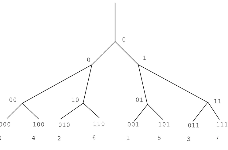
Consider a N-generation dyadic tree. Nodes of a given generation are indexed as shown in Fig. 3: starting from the root, a right turn is encoded by 0, a left turn by 1. A node at generationN is represented byN bits: aN−1aN−2. . . a0. We map thisN−bit number onto Z/2nZin the following manner
aN−1aN−2. . . a07−→
N−1
X
k=0
ak2k
considered as a element of Z/2N
Z. This leads to an indexing of the boundary (set of leafs) ΓN of the N
generation 2-adic tree, that is more natural, as we shall see, than the linear indexing 0, 1, 2, . . . . For instance, the indexing for N = 3 is the following: 0, 4, 2, 6, 1, 5, 3, 7. Now anya ∈Z/2N
Z can be writtena=a02p,
with a0 odd. We definep=p(a)∈[0, N−1] as the valuation of a. The 2-adic absolute value ofa is defined as |a|2= 2−p(a). The 2-adic distance between two verticesaandbof ΓN (identified toZ/2NZ) is then defined
as |b−a|2. This distance reflects the tree structure, in the sense that it is a monotone function of the graph-distance between vertices, defined as the length of the shortest path (in the tree) connecting two vertices of ΓN.
In particular, the distance is minimal (1/2N−1) when 2 leafs share a direct ascendant, and maximal (equal to
0
0
1
00
10
01
11
000
100
010
110
001
101
011
111
0
4
2
6
1
5
3
7
Figure 3. 2-adic indexing
functiongin RΓN (that can be seen as a 2N dimensional vector), we shall write
Z
Z/2NZ
g(x)dx= 1 2N
2N−1
X
k=0
g(k),
in the spirit of Haar’s measure onZ2, the ring of 2-adic integers (see [4]). The underlying measure is such that
a set of the formz+ 2 Z/2NZ, has total measure 1/2. Similarly, the set z+ 2p Z/2NZhas a measure 1/2p,
forp≤N, for anyz.
Proposition 2.8. Consider a symmetric N-generation dyadic tree (i.e. the resistance is the same for all branches of the same generation). The resistance operator defined in a general setting by Def. 2.6, and for dyadic trees by the matrix (16), can be written
p(x) =Rq(x) =
Z
Z/2nZ
Ψ(x−y)q(y)dy. (17)
Proof. This is a direct consequence of the matrix expression (16), in the case where the resistance does not depend on the branch within each generation, i.e. rk
n ≡rn. Consider for instance a flux vector that is 1 at 0,
and 0 at all other vertices . For all those vertices that are not in the same half than 0, the pressure is simply r0. For all those that are in the same half, but not in the same quarter, the pressure isr0+r1, etc. . . In the
2-adic setting it suffices to define Ψ by
Ψ : x∈Z/2NZ7−→Ψ(x) =r0+r1+· · ·+rk, with k=−log2(|x|2),
2.5.
Stochastic setting
We briefly describe here the links between the discrete Laplace problem and a stochastic process. Further details about this setting can be found in [7]. This section is purely abstract in the sense that the random walk that we will describe is not related to any actual process in the physical space, but it enlightens the mathematical structure of the problem, and it can be used to compute equivalent resistances by a Monte Carlo algorithm.
Considering a NetworkN = (V, E, r), we define a random walk by the transition probabilitiesπxy, wherex
andy range over the set of vertices. This transition probability is defined as
πxy=
c(x, y)
C(x) , C(x) =
X
y∼x
c(x, y), (18)
where c(x, y) = 1/r(x, y) is the conductance of edge (x, y). The probability to go fromx toy is 0 as soon as y is not connected tox. The corresponding Markov chain is irreducible as soon as the network is connected, which we assume here.
Now consider a rooted networkN = (V, E, r, o,Γ) and Dirichlet data on Γ: a collection of values (P(x))x∈Γis
prescribed. We definep∈RV as follows: considering a vertexx∈V, we denote byithe step that corresponds
to the first hitting with Γ oroof the random walk starting fromx:
X0=x , X1, . . . , Xi∈Γ∪ {o},
withXj ∈/ Γ∪ {o} for 0< j < i. The value ofP at Xi (it is zero wheneverXi=o) is a random variable. We
denote byp(x) the corresponding expected value. We have the following link between this process and Dirichlet Problem (11).
Proposition 2.9. Let p∈RV be defined as previously. Then pis the solution to Problem (11).
Proof. Let us first notice that Dirichlet boundary conditions are automatically verified (in the casex∈Γ∪ {o}, the first hitting indexiis 0). Now consider x∈V˚. It holds
p(x) =X
y∼x
πxyp(y),
which can be written (from (18))
C(x)p(x)−X
y∼x
c(x, y)p(y) = 0,
so thatpis harmonic. As a consequence, it is the unique solution to (11).
This property can be used to obtain a stochastic expression of the resistance betweenoand Γ. Consider the case whereP ≡1. The field pdefined previously is then the escape probability: for x∈V, it represents the probability that the random walk starting fromxhits Γ (i.e. “escapes”) before hitting Γ.
Proposition 2.10. Consider a random walk starting fromo, transition probabilities given by (18). It holds 1
R =C(o)pesc, (19)
Proof. Letpbe the solution to the Dirichlet problem (11). By Definition 2.3, the resistanceR is 1/d(o). Now by Prop. 2.9, the escape probability is
pesc=
X
x∼o
πoxp(x) =
1 C(o)
X
x∼o
c(o, x)(p(x)−p(o)) = 1
C(o)du(o) = 1 C(o)
1 R,
which yields the result.
2.6.
Actual computation of the equivalent resistance for a general dyadic tree
The actual computation of the equivalent resistance of a network is dictated by Def. 2.3. It amounts to solving the discrete Dirichlet problem (11), withP ≡1, and then compute the resistance asR= 1/du(o). In the case of aN-generation dyadic tree, an alternative approach can be undertaken, by means of the resistance operatorR, defined in matrix form by (16). Consider a unit pressure field p= (1,1, . . . ,1)∈R2
N , solve
Rj=p,
and then compute the total flux as the sum of elements of j. The advantage is not obvious, since the straight approach consists in solving a 2N+1×2N+1 system for a verysparsematrix (the maximal number of non-zero
entries in a row is 4), whereas the Neuman-Dirichlet approach that we propose here consists in solving a slightly smaller linear system (2N×2N), but with afullmatrixR. Yet, the particular structure ofR, (see (16)), makes
it possible to design a fast matrix-vector product. We describe the idea of the method for the linear indexing (that corresponds to the matrix expression (16)), but it could be also be formulated within the 2-adic setting presented in Section 2.4. For a given flux field q, the matrix-vector product R requires the computations of partial sums
q0+q1, q2+q3, q4+q5, . . .
and then
q0+q1+q2+q3, q4+q5+q6+q7, . . . etc
Once the 2-term sums have been computed, it is clear that each 4-term sum only requires a single addition (and not 3). Recursively computing those sums to perform the matrix-vector product leads to a very efficient algorithm. The linear system can then be solved by an iterative algorithm, like the conjugate gradient algorithm. Note that a Monte Carlo method can also be undertaken in the spirit of Section 2.5, according to Formula (19). This approach is less accurate than the direct one (described previously), but it can be useful in the case where some individual resistances are very large. Indeed, the large condition number of the matrix is likely to harm the convergence speed of any iterative method, while it will not affect the behavior of the Monte Carlo strategy. We refer to [16] for a detailed comparison of both approaches, in various situations.
3.
Optimality and stability issues
This section addresses natural questions concerning optimality and robustness of the lung as a resistive tree, both from the standpoint of constrained optimization and from the statistical standpoint.
3.1.
Minimizing the cost of breathing
There is an increasing number of research papers dedicated to optimality of physiological systems. We must stress out that the answer to the question:
Is the system optimal ?
required tidal volume (see Section 1), an obvious criterium is the energy cost. A first attempt in this direction was proposed in [13].
The authors consider aN-generation dyadic tree that is assumed to be symmetric. They furthermore assume that all branches over the tree have the same aspect ratio: if`n is the length at generation n, the diameter is
c`n, so that the individual resistance of a branch linearly depends on 1/`3n, see Eq. (9). To alleviate notations,
we shall consider that the resistance of a pipe at generationn is simplyrn= 1/`3n (we drop the multiplicative
constant). Similarly, each branch at generation n occupies a volume `3
n. For a unit flow rate, the dissipated
power reduces to the global resistance (see Prop. 2.4), that is
P =R=
N
X
n=0
1 2n`3
n
.
whereas the total volume is
V =
N
X
n=0
2n`3n.
Considering that the volume is subject to remain below a maximal value, minimization of the resistance under this constraint can be solved exactly.
Proposition 3.1. (From [13])
Under the previous assumptions, minimality of R under the maximal volume constraint is achieved for a geo-metric progression of the sizes, i.e.
`n =βλn, with λ= 2−1/3,
whereβ is a normalization constant which ensures that the volume constrained is saturated.
Proof. This is a straightforward application of the Kuhn-Tucker necessary conditions for optimality under
constraint.
This academic result is quite striking, since it can be assessed from actual measurements (see [24], or Table 1 taken from [23]) that the progression is indeed not far from being geometric, at least in the central range of generations (i.e. from 3 to 16). Furthermore, the measured value, that is 0.85, is quite close to the “ideal” one 2−1/3≈0.79. We refer the reader to [13] for further discussions on the gap between the two values.
Note that the constrained optimization can be set in a different manner, by disregarding the maximal volume constraint, and replacing it by a constraint based on lengths. Assuming that the entrance of the respiratory system is necessary at a prescribed distance of the zone it is meant to irrigate, we may consider that the length of any path from the root to the leaf is fixed, i.e.
`tot= N
X
n=0
`n
is prescribed. It can be shown with similar arguments (see [16]) that the optimum still exhibits a geometric character, with a ratio 1/√4
2≈0.84 that is even closer to the experimental one.
Proposition 3.2. Among all those pressure fields on V that vanish at o, harmonic over the set of interior vertices˚V =V \({o} ∪Γ), and driving a unit flux through o(or, equivalently, the opposite flux throughΓ), the one that minimizes the dissipated energy is uniform over Γ.
Proof. Let us denote byH the set of pressure fields that vanish at 0. The problem consists in minimizing
1 2
X
e∈E
c(x, y) (p(x)−p(y))2.
over
q∈H01, dcd?q(o) = 1 , withH01=
q∈RV , q(o) = 0.
By global conservation (see (14)), the flux constraint can be written (with u=−cd?q)
1 =dcd?q(o) =−du(o) = +X
x∈Γ
du(x) =−X
x∈Γ
dcd?p(x).
The problem can be set as a saddle point-problem (see e.g. [6]): it amounts to find a couple (p, λ)∈H1 0 that is
a saddle-point for the Lagrangian
L(q, µ) =1 2
X
e∈E
c(x, y) (q(x)−q(y))2+λ X
x∈Γ
dcd?q(x) + 1
!
The optimality conditions for the primal component write in a variational way as
X
e∈E
c(x, y) (p(x)−p(y)) (q(x)−q(y)) +λX
x∈Γ
dcd?q(x) = 0 ∀q∈H01, harmonic on ˚V .
Applying properly the discrete Green formula (13) to the first term, we obtain
X
x∈V˚
p(x)dcd?q(x) +X
x∈Γ
p(x)dcd?q(x) +λX
x∈Γ
dcd?q(x) = 0 ∀q∈H01.
Now for any collection of fluxesj∈RΓ (extended by 0 for vertices in ˚V), we may consider the solutionq∈H1 0
to
dcd?q(x) =j(x) ∀x∈V˚∪Γ. Plugging this very field in the variational formulation above leads to
X
x∈Γ
(p(x) +λ)j(x) = 0.
Sincej can be chosen arbitrarily, it implies that p≡ −λon Γ, hence the pressure field is uniform.
3.2.
Resistance dispersion and generation-wise Sobol sensitivity indices
Table 1. Lengths and diameters, with relative variations (from [23])
Generation Length (mm) σ/m Diam. (mm) σ/m
0 105 0.1 15.7 0.1
1 41.6 0.15 10.1 0.1
2 16.6 0.25 7.3 0.125
3 6.6 0.3 4.9 0.175
4 11.1 0.35 3.9 0.2
5 9.4 0.425 3.1 0.23
6 7.9 0.5 2.5 0.275
7 6.7 0.575 2.0 0.325
8 5.6 0.65 1.6 0.35
9 4.7 0.70 1.35 0.42
10 4.0 0.75 1.14 0.5
11 3.4 0.80 0.95 0.575
12 2.9 0.81 0.83 0.66
13 2.4 0.775 0.72 0.675
14 2.0 0.725 0.65 0.6
15 1.7 0.65 0.58 0.5
Beside mean values, the table indicates coefficients of variation. Those are defined as the dimensionless ratio of standard deviation and mean value. They progress along the tree from small values (about 10 %) to much higher values (about 80 % for generations 11 and 12). The variability that can be induced for the resistance of individual branches is huge. Consider for exemple a branch at generation 10, assume that its diameter and its length are (independent) random variables that follow a log-normal law, with mean values and standard deviations given by Table 1. The corresponding resistance can be considered as a random variable. The mean and the standard deviation can be estimated as
r10= 222 cm H2O s L−1, σ10≈1400cm H2O s L−1.
Note that the mean value is more than 100 times the resistance of the overall tree. Furthermore, the coefficient of variation of the individual resistance is about 600 %. We aim here at investigating the real effect of this huge individual variability upon the global resistance.
We denote byXn the vector of lengths and diameters of the 2n branches of generationn:
Xn= (`0n, `1n, . . . , `2 n−1
n , d0n, d1n, . . . , d2 n−1 n ).
The global resistance R can be written as a function of the geometric characteristics (lengths and diameters) of all branches, i.e.
R=R(X0, X1, X2, . . . , XN).
Following [23], we now assume that all diameters and lengths are independent random variables, so that R is itself a random variable. Table 1 gives experimental values for the lengths and diameters of the branches over the generation range, together with associated coefficients of variation (dimensionless number, defined as the standard deviation divided by the mean value). Following [23] again, we shall consider each geometric parameter follows a log-normal distribution. Let us consider one of those variables (length or diameter at some generation n), denoted byX, with meanmand standard deviationσ. It consists in writing
0.38 0.4 0.42 0.44 0.46 0.48 0.5 0.52 0.54 0.56 0
0.02 0.04 0.06 0.08 0.1 0.12 0.14
resistance
Figure 4. Resistance distribution
whereN is a normal law with meanµand standard deviationτ, with
µ= log p m 1 +σ2/m2
!
, τ =
s
log
1 + σ
2
m2
.
We shall therefore consider that all geometric quantities `k
n anddkn follow such laws, the parameters of which
only depends on generation indexn, and that all random variables are independent.
Actual computation of equivalent resistances associated to randomly generated trees can be performed (see section 2.6), and Fig. 4 shows the obtained histogram (with 30000 samples). Two remarks are in order. First, the mean value (0.47 cm H2O s L−1) is significantly higher that the value computed for the symmetric tree,
with the mean values given by Table 1 (0.28 cm H2O s L−1). Second, the distribution is narrow: the standard
deviation is 0.02, that is about 4% of the mean value. This asserts the strong robustness of the tree resistance with respect to the variability of constitutive parameters.
We now aim at quantifying the role played by the variability within each generation upon the global variability of the resistance, by means ofSobol sensitivity indices(see e.g. [22]). In this spirit, for anyn, anyXn, we define
Rn(Xn) as
Rn(Xn) =E(R(X)|Xn).
This quantity is a random variable that depends on Xn only. We denote byσn2 its variance. The n−th Sobol
index is then defined as
Sn=
σ2
n
σ2,
where σis the standard deviation of R. This dimensionless indexSn, between 0 and 1, quantifies the part of
the global variance that isexplainedby generationn.
Estimation ofSn. For any generationn, the indexSncan be estimated by means of a Monte Carlo algorithm.
It is based on generating samplings of the full vector of parameters
X = (X0, X1, . . . , Xn−1, Xn, Xn+1, . . . , XN),
together with samplings of
X0 = (X00, X10, . . . , Xn0−1, Xn, Xn0+1, . . . , XN0 ).
It holds
Sn=
cov(R, R0)
var(R) , withR=R(X), R
0 =R(X0).
LetR1, R2, . . . ,R01,R02, . . . be the sampled values. The Monte Carlo approach is then based on the following
estimator (see [10]):
ˆ Sn=
1
K
PK
k=1RkR0k−
1
K
PK
k=1Rk K1 P K k=1R0k
1
K
PK
k=1(Rk)
2
−1
K
PK
k=1Rk
2 .
The results are presented in Fig. 5, for K = 10000 samples for each generation. The standard deviations for each index (represented in the figure) is estimated by bootstrapping (random sampling with replacement from the same sample set of values for R, R0). It appears that the largest part of the variability is due to the proximal generations (generations 0 to 8), whereas further (distal) generations play essentially no role in this variability. Another striking fact is the balanced distribution of indices in the proximal part: they vary between 0.05 and 0.15. It suggests that evolutionary principles might tend to equi-distribute variability contributions in some complex systems like the respiratory tract.
4.
Conclusion
Starting from the Top-Down (or functionalist) notion of resistance as a single scalar that can be measured from the outside, we described here frameworks that have been elaborated to properly define such a notion at a mathematical level. This approach makes it possible to handle the whole geometric complexity of the respiratory tract. We acknowledge the apparent futility in the process: considering a living subject, a full and accurate knowledge of geometric characteristics of his/her respiratory tract is clearly out of reach. Yet, computing equivalent resistances for general (i.e. non-symmetric) trees makes it possible to investigate the effect of microscopic variability (at the level of individual branches) over the global resistance. The main outcomes of these direct computations are
(1) The variability of individual branch characteristics has a significant effect upon the mean value of the effective resistance. As we pointed out in Section 3.2, the effective mean value is about twice the resistance computed from the mean geometric parameters.
−2 0 2 4 6 8 10 12 14 16 −0.05
0 0.05 0.1 0.15 0.2
Generation
Sobol index
Figure 5. Sobol indices
(3) As for the respective contributions of the branches upon the global variability, Sobol analysis exhibits two distinct zones: a proximal one (branches 0 to 7 or 8), in which the contribution to global variability is fairly uniformly distributed over generations, and a distal one (generation 9 and above), that corresponds to generations which do not significantly contribute to variability.
All these arguments tend to support the relevance of the resistance as a lumped parameter. The respiratory tract as a resisitive network remains a complex system, but this complexity is in someway smoothed by nonlinear interactions between parameters, and the tree structure provides a great robustness to the overall process.
References
[1] A. Ben-Tal,Simplified models for gas exchange in the human lungs, J. Theor. Biol.238(2006), 474–495.
[2] R. Carlson, Myopic models of population dynamics on infinite networks, Networks And Heterogenous Media , Volume 9, Number 3, September 2014.
[3] J.E. Cotes, D.J. Chinn, M.R. Miller,Lung Function, Blackwell 2006.
[4] F. Bernicot, B. Maury, D. Salort,A 2-adic approach of the human respiratory tree, Netw. Heterog. Media 5 (2010), no. 3, 405–422.
[5] S.-Y. Chung, Y.-S. Chung, J.-H. Kim,Diffusion and Elastic Equations on Networks, Publ. RIMS, Kyoto Univ. 43 (2007), 699?726.
[6] P.G. Ciarlet,Introduction to Numerical Linear Algebra and Optimisation, Cambridge Texts in Applied Mathematics (Book 4), Cambridge University Press (1989).
[7] P. Doyle, J. L. Snell,Random Walks and Electric Networks, Mathematical Association of America, 1984.
[9] R.H. Ingram, T.J. Pedley,Pressure-flow relationship in the Lungs, in Comprehensive Physiology, supplement 12: Handbook of Physiology, The respiratory system, mechanics of breathing, 2011, 277-293.
[10] A. Janon, T. Klein, A. Lagnoux, M. Nodet, C. Prieur,Asymptotic normality and efficiency of two Sobol index estimators, 2012. Accepted in ESAIM: Probability and Statistics.
[11] M. Kramar Fijavˇz, D. Mugnolo, E. Sikolya,Variational and Semigroup Methods for Waves and Diffusion in Networks, Appl Math Optim 55:219–240 (2007).
[12] B. Mauroy, N. Meunier, Optimal Poiseuille flow in a finite elastic dyadic tree, ESAIM : M2AN , 42, 507-534, July-August 2008.
[13] B. Mauroy, M. Filoche, E. R. Weibel, and B.Sapoval,An optimal bronchial tree may be dangerous, B. Mauroy, Nature, 427, 633-636, 12 February 2004.
[14] B. Mauroy, M. Filoche, J.S. Andrade Jr., B. Sapoval, Interplay between flow distribution and geometry in an airway tree, Phys. Rev. Lett. 90,14(2003).
[15] B. Mauroy and P. Bokov,Influence of variability on the optimal shape of a dichotomous airway tree branching asymmetrically, Phys. Biol., 7:016007 (2010).
[16] B. Maury,The Respiratory System in Equations, (MS& A), ed. Springer, 2013.
[17] B. Maury, D. Salort, C. Vannier,Trace theorems for trees, application to the human lung, Network and Heterogeneous Media, Volume 4, Number 3, September 2009, 469–500.
[18] Pedley, T.J., R.C. Schroter, and M.F. Sudlow,The prediction of pressure drop and variation of resistance within the human bronchial airways, Respir Physiol, 1970. 9(3): p. 387–405.
[19] T. Ritz, B. Dahme, A.B. Dubois, H. Folgering, G.K. Fritz, A. Harver, H. Kotses, P.M. Lehrer, C. Ring, A. Steptoe, and K.P. Van de Woestijne,Guidelines for mechanical lung function measurements in psychophysiology, Psychophysiology, 39 (2002), 546–567.
[20] Fritz Rohrer,Der Str¨omungswiderstand in den menschlichen Atemwegen und der Einfluss der unregelm¨assigen Verzweigung des Bronchialsystems auf den Atmungsverlauf in verschiedenen Lungenbezirken, Pfl¨uger’s Archiv f¨ur die gesamte Physiologie des Menschen und der Tiere 28. Oktober 1915, Volume 162, Issue 5-6, pp 225-299.
[21] P. M. Soardi,Potential Theory On Infinite Networks, Springer-Verlag (1994).
[22] I.M. Sobol’,Global sensitivity indices for nonlinear mathematical models and their Monte Carlo estimates, Mathematics and Computers in Simulation 55 (2001) 271–280.
[23] T.T. Soong, P. Nicolaides, C.P. Yu, S.C. Soong,A statistical description of the human tracheobronchial tree geometry, Respir Physiol. 1979 Jul;37(2):161-72.
[24] E.R. Weibel,Morphometry of the human lung, Springer Verlag and Academic Press, Berlin, New York, 1963. [25] E.R. Weibel,The Pathway for Oxygen, Harvard University Press, 1984.
[26] I. Weinhold, G. Mlynski,Numerical simulation of airflow in the human nose, Eur Arch Otorhinolaryngol. 261:452-455, 2004. [27] J. Wen, K. Inthavong, J. Tu, S. Wang,Numerical simulations for detailed airflow dynamics in a human nasal cavityRespir.
Physiol. Neuro. 161:125-135, 2008.
![Table 1. Lengths and diameters, with relative variations (from [23])](https://thumb-us.123doks.com/thumbv2/123dok_us/10067294.1993093/18.612.152.416.143.356/table-lengths-diameters-relative-variations.webp)