Modelling and analysis of protein aggregation - Competing pathways in prion (PrP) polymerisation*

J.-S. Dhersin, Editor

MODELLING AND ANALYSIS OF PROTEIN AGGREGATION - COMPETING

PATHWAYS IN PRION (PRP) POLYMERISATION

Wafaˆ

a Haffaf

_{and St´}

_{ephanie Prigent}

Abstract. Protein aggregation leading to the formation of amyloid fibrils is involved in several neu-rodegenerative diseases such as prion diseases. To clarify how these fibrils are able to incorporate additional units, prion fibril aggregation and disaggregation kinetics were experimentally studied using Static Light Scattering (SLS). Values that are functions of P

i≥1

i2_ci, with ci being the concentration of fibrils of size i_{, were then measured as a function of time. An initial model, adapted from the} Becker-D¨oring system that considers all fibrils to react similarly is not able to reproduce the observed in vitro _{behaviour. Our second model involves an additional compartment of fibrils unable to} incor-porate more prion units. This model leads to kinetic coefficients which are biologically plausible and correctly simulates the first experimental steps for prion aggregation.

R´esum´e. L’agr´egation des prot´eines conduisant `a la formation de fibres amylo¨ıdes est impliqu´ee dans plusieurs maladies neurod´eg´en´eratives telles que les maladies `a prion. Pour clarifier la mani`ere dont les fibres de prion incorporent des unit´es suppl´ementaires, les cin´etiques d’agr´egation et de d´esagr´egation des fibres ont ´et´e ´etudi´ees exp´erimentalement (par SLS, “Static Light Diffusion“). Ainsi des valeurs fonction de P

i≥1

i2_ciavec cila concentration en fibres de tailleiont ´et´e obtenues en fonction du temps. Un premier mod`ele, adapt´e du syst`eme de Becker-D¨oring, qui consid`ere que la totalit´e des fibres r´eagit de mani`ere similaire ne permet pas de reproduire le comportement observ´ein vitro. Notre deuxi`eme mod`ele met en jeu un compartiment additionnel de fibres incapables d’incorporer davantage d’unit´es de PrP. Celui-ci aboutit `a des coefficients cin´etiques biologiquement plausibles et simule correctement les premi`eres ´etapes exp´erimentales de l’agr´egation de prions.

Introduction

More than twenty diseases, known as amyloid diseases and which include Alzheimer’s, Hungtington’s and prion diseases are due to the conversion of a protein structure into a misfolded conformation that induces pro-tein aggregation. Recent studies have shown that injections of aggregated propro-teins involved in Alzheimer’s and Parkinson’s diseases follow a prion-like mechanism behaviour by a cell-to-cell transmission [6]. However, the exact mechanisms for incorporating prion (PrP) protein to a prion aggregate remain to be clarified. To better

∗_{The authors would like to warmly thank the head of this project, Marie Doumic-Jauffret (INRIA), for her major contribution}

to this work and Human Rezaei, Davy Martin (INRA) and Joan Torrent Y Mas (INSERM) for initiating this topic, the

experimental part and discussions. This research was supported by the ERC Starting Grant SKIPPERAD_{(fully for S. Prigent}

and partially for W. Haffaf ).

1_{Inria, Paris-Rocquencourt, Domaine de Voluceau, BP105, 78153 Le Chesnay, France; LJLL, Laboratoire Jacques-Louis Lions,} Pierre et Marie Curie University, Boite courrier 187, 75252 Paris Cedex 05, France)

2 _{Inria; LJLL; INRA, VIM, Domaine de Vilvert, 78352 Jouy-en-Josas cedex, France}

c

EDP Sciences, SMAI 2014

understand how PrP fibrils can recruit PrP molecules that were not misfolded, we have studied the kinetics of PrP fibril elongation, focusing on polymerisation through the addition of monomer(s) on fibrils. A loss of fibril ability for further polymerisation was experimentally observed after a given number of additions of monomers. Among several hypothetical mechanisms and according to different experiments [7], a hypothetical occurrence of a structural defect on fibrils could explain this loss of the ability to polymerise.

Relying on the iterative modeling process, we have written two models for the simulation of prion polymerisa-tion/depolymerisation. The first model, the basic one, led us to the Becker-D¨oring system for phase transition phenomena. Nevertheless, this model was unable to reproduce the loss of fibril ability for polymerisation. The second model involves the formation of fibrils with a structural defect preventing them from any further poly-merisation. This model, with suitable parameter estimations, numerically reproduces part of the empirically observed curves of prion fibril kinetics.

1.

Biological experiments

To clarify prion aggregation mechanisms, polymerisation and depolymerisation of prion fibrils were studied in vitro as a function of time, starting from preformed fibrils. These experiments were set up and performed by the team of Dr. H. Rezaei, Dr. D. Martin and Dr. J. Torrent Y Mas from INRA (Jouy-en-Josas, France). The kinetics were followed by SLS (Static Light Scattering) performed on a cuvette containing PrP fibrils in an aqueous buffer solution. SLS measures α(P

i≥1

i2_c

i) +β, with ci being the concentration of polymers of size i,

andαand β being parameters that are constant during each experiment. Because the experimental sample is a heterogeneous mixture of polymers of various sizes, this technique does not give access to the concentration of polymers of a precise size. To clarify the mechanisms involved in fibril growth once fibrils have formed, i.e. how additional monomers are recruited by fibrils, the experimental approach consisted in successive additions of monomers on fibrils (Figure 1). At time 0 a first addition of monomers was performed on the fibrils. The following additions of monomers were made once the SLS measurement had reached a quasi plateau. After a certain number of additions of human PrP monomers on human PrP fibrils, the SLS signal did not increase anyfurther. However, the SLS signal was increased by a further addition of mutant PrP monomers that differ from human PrP monomers in their structure. This observation and other experiments indicate that fibrils growth probably does not stop simply because the fibril has reached a certain size [7].

Complementary experiments using another technique (spectrophotometry) were also performed to get a crude estimate of the concentration of free monomers at the end of the first two plateaux; these indicated that only a small percentage of initial monomers was incorporated onto fibrils.

0 50 100 150 200 250 300

30 35 40 45 50 55 60

Time (min)

SLS intensity

2.

Basic model for fibril-monomer reaction

We start this modeling process by considering only classic prion fibrils with their basic reactions, which results in the following model.

2.1.

Basic model

An i-sized polymer can gain a free monomer to become an (i+ 1)-sized polymer. This reaction is called polymerisation, it occurs with a non-negative size-dependant rate koni.

An i-sized polymer can also release a monomer, giving rise to a smaller polymer, of size i−1, and a free monomer. This reaction is named depolymerisation. It occurs with a non-negative size-dependant rate, kdepi. Denoting by ci the concentration in polymers of sizei, withi= 1,2, ..., we get the following scheme of reactions:

ci+ c1 koni

−→ ci+1, i≥1,

ci −→

kdepi

ci−1+ c1, i≥2.

In terms of equations, it gives the well-known Becker-D¨oring system [2] :

  

 

dci

dt =−konic1ci+ koni−1c1ci−1−kdepici+ kdepi+1ci+1 i≥2,

dc1

dt =−

∞

P

i=2

konic1ci−kdepi+1ci+1

−2 kon1c

2

1−kdep2c2

. (1)

This is obtained directly from the schemes reactions, using the law of mass action several times. One can notice that a particular equation is needed for the variation of concentration of 1-sized particules that are called monomers. This is due to their interaction in all the processes.

A detailed qualitative study of this system was carried out in several articles, such as [1], [3], and [5]. In [1], the authors give theorems of existence, uniqueness, continuous dependence of initial data and the fundamental mass conservation property:

c1(t) = ∞

X

i=1

(ici(0))−

∞

X

i=2

(ici(t)).

For new fibrils to be created through the reaction

c1+ c1 k_on1

−→ c2

biogically requires a greater time than the time-scale of the experiments reported here. This was deduced through a control experiment where a constant signal was observed when using only monomers in the same duration (300min). Therefore, the coefficient kon1 is assumed to be null (kon1 = 0).

2.2.

Simplified system

To gain further qualitative insight into the dynamics of these equations and a concrete idea about the order of magnitude of the kinetics coefficients konand kdep, we initially consider a simplified system (which we will make

more complex afterwards). This involves a summation of all the equations of the infinite Becker-D¨oring system (1) over all sizes. The simplification is the assumption we make on the coefficients konand kdepby considering

them to be constant. As all the fibrils are almost the same size, this assumption is justified. Moreover, we consider a time-scale where the concentration in dimers, c2, is negligible. This results in the following simplified

             dP

dt = 0 dM

dt = konc1P−kdepP dc1

dt =−konc1P + kdepP

(2)

where P = P

i≥2

ci(t) represents the total concentration of fibrils summed over all sizesi≥2,

M = P

i≥2

ici(t) represents the total mass of fibrils summed over all sizesi≥2,

c1 the concentration of monomers.

The total mass conservation is then obvious.

The equation of the second order moment (measured data) variation is also simplified into :

dMmeasured2

dt = 2M (konc1−kdep) + 2kdepP

and once the closed simplified system (2) has been solved, an analytical expression for Mmeasured

2 can be easily

deduced. Indeed, after integrating (2) we get :

      

P = Pin

M (t) = Min−kon cin1 −c

eq

1

e−konPint_Pin_{+ c}in

1 −c eq 1

c1(t) = cin1 −c

eq

1

e−konPint_{+ c}eq

1

(3)

where Pin _{= P (0) represents the initial total concentration of polymers and M}in _{= M (0) their initial total}

mass, cin

1 = c1(t= 0) the initial concentration of monomers and ceq1 = kdep

kon the concentration of monomers at

equilibrium state (when dc1

dt = 0, see (2)).

Thus,

Mmeasured2 =A+B(e−konP

in

t

−1) +C(e−2konPint_{−1) + 2k}

depPint,

withA= Min2 , B=−P2in(M

in

+ cin

1 −c

eq

1 )(cin1 −c

eq

1 ) andC= (ceq

1 −c in 1 )

2

Pin .

One can notice from the mass expression M (t) above that we need to assume ceq₁ = kdep

kon ≤ c

in

1 + Min, else

neglecting c2 in (1) is not valid and M (t) defined by (3) would become negative for large time.

The next step is then to estimate the parameters kon, kdep, αandβ using the experimental data ofSLS with

SLS =αMmeasured

2 +β.

We reformulate this inverse problem into the minimisation of the corresponding least squares criterion

J(kon,kdep, α, β) =

n X i=1

αMmeasured2 (ti; kon,kdep) +β

−SLS(ti)

2

The uniqueness of the solution is, as for most non-linear inverse problems, non-trivial. This is essentially due to the non-convexity of thecost functional J.

0 10 20 30 40 50 60 70 34

35 36 37 38 39 40 41 42 43 44

Time (min)

SLS

Raw Data

Denoised Data (Wavelet Transform) Simulations

0 20 40 60 80 5.814

5.814 5.814 5.814 5.814x 10

−10

The total concentration of all fibrils

Time(min) 0 20 40 60 80

2 4 6 8 10 12x 10

−7

The total mass of all fibrils

Time(min)

0 20 40 60 80 4

4.2 4.4 4.6 4.8

5x 10

−6

The monomer concentration

Time(min)

0 20 40 60 80 5.2

5.2 5.2 5.2 5.2x 10

−6

The total mass of all fibrils + Monomers

Time(min)

Figure 2. _{Simulation of the first addition of monomers. (Quantities are inmol.L}−1_.)

the first step ( due to volume dilution in the cuvette), the gap between two successive additions is higher and

higher (Figure 3). This is due to thei2 _{term in the simulated quantity α(}Pn

i≥1

i2_c

i) +β (Figure 3).

0 20 40 60 80 100 120 140 160 180 200 0

0.05 0.1 0.15 0.2 0.25

Time(min)

Sum (i

2 c

i

) + Monomers

Monomer Addition

Monomer Addition

0 20 40 60 80 100 120 140 160 180 200 4

5 6 7 8 9 10x 10

−6

Time(min)

c

1

(t)

Monomer Addition Monomer Addition

Figure 3. _{Simulation of the first three additions of monomers with solute-dilution in the}

We conclude here that a stop pathway is needed to slow down the polymerisation of fibrils and the growth of their average sizeiand, hence,i2_.

3.

Two-compartment model

3.1.

Discrete model

To force the polymerisation to stop, we set the hypothesis of creating a different fibril that will no longer be able to polymerise due to a defect in its structure.

Thisdefective fibril would be the result of the polymerisation of aclassic fibril with a polymerisation rate kmon.

We denote by cm

i the concentration of the defective fibrils of sizei. The reactions are now:

ci+ c1 koni

−→ ci+1, i≥1,

ci −→

kdepi

ci−1+ c1, i≥2,

ci+ c1 km

oni

−→ cmi+19, i≥2,

cm

i −→

km depi

ci−1+ c1, i≥3.

Which can be translated into the following ordinary differential equations system :

                          

dci

dt =−konic1ci+ koni−1c1ci−1−k m

onic1ci−kdepici

+ kdep_i+1ci+1+ kmdepi+1c

m

i+1, i≥2

dcm

i

dt = k

m

oni−1c1ci−1

−kmdepic

m

i , i≥3

dc1

dt =−

∞

X

i=2

konic1ci− ∞

X

i=2

kmonic1ci+ ∞

X

i=2

kdepici+ ∞

X

i=3

kmdepic

m

i

−2 kon1c

2

1−kdep₂c2

3.2.

The two-compartment simplified system

We denote by Pm=P

i≥3

cmi (t) the total concentration of defective polymers.

Mm= P

i≥3

icm

i (t) the total mass of defective polymers.

Summing once again over all sizes, we obtain the following system :

                               dP

dt =−k

m

onc1P + kmdepPm

dPm

dt = k

m

onc1P−kmdepPm

dM

dt = konc1P−k

m

onc1M−kdepP + kmdep(Mm−Pm)

dMm

dt = k

m

onc1(P + M)−kmdepMm

dc1

dt =−konc1P−k

m

onc1P + kdepP + kmdepPm

and the measured data :

dMmeasured2

dt = 2c1M (kon+ k

m

on) + 2kdep(P−M) + 2kmdep(Pm−Mm) (5)

In order to fit the experimental data for the first addition of monomers, kinetic parameters for the two-compartment model were obtained as follows.

We suppose the fibrils to be exclusively composed of classic fibrils at time 0, and that defective fibrils are absent. We start with a simplified view of the system to obtain certain values of kinetic constants able to fit the data. For this reason, we consider that at the beginning of the experiment the system is nearly a model with only one compartment.

For the basic model, we can deduce from (3) that after a certain time denotedteq _{(for equilibrium time), the}

quantity cin

1 −c

eq

1

e−konPinteq _{is negligible when compared to c}eq

1 . We considere−konP

in

teq _{in the 10}−1 _range,

i.e. −konPinteq≃ −2. Therefore, for the basic model, we have approximately :

konPinteq= 2

⇒ kon=

2 Pinteq

(6)

By analogy with the basic model, after replacing Pin(P initial) by Peq(P of classic fibrils at equilibrium state) in the konformula (6) from the basic model, we can obtain certain values of konand kdep, for the two-compartment

model, able to fit the first minutes. To calculate kon, we use a fixed value for teq = 8 min (chosen from the

minimal time where the experimental SLS slope reaches nearly 0). For kdep, with kdep= konceq1 ,we use 10075c

in

1 ≤c

eq

1 ≤ 10096c

in

1 (from experimentally estimated values of c1) where

cin

1 = 5.10−6mol.L−1.

In this way, during the first minutes, the concentration of consumed c1is modulated by the classic fibrils (more

exactly by the ratio kdep/kon) whereas any effect of the few defective fibrils on the concentration of monomers

can be ignored. This analogy with the ’basic model’ offers access to a part of the sets of plausible kinetic constants able to fit the first addition of monomers.

Once kon and kdep were calculated as functions of Pm

eq

(the concentration of defective fibrils at equilibrium state, with a value from 0 to 100 % of Pin_{), the kinetic constants k}m

dep and then kmon for defective fibrils were

deduced. kmdepwas got by a small inverse problem (using the Matlab routine fminsearch) from a broad range of

potential kmdepvalues (0≤kmdep≤104).

kmonwas deduced from the equilibrium state between classic and defective fibrils:

dP

dt =

dPm

dt = 0 ⇒ −k

m

onc1P + kmdepPm= 0

⇒kmon=

kmdepP m

c1P

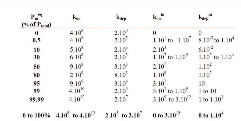
Table 1 presents calculated values for the kinetic parameters allowing us to reproduce the SLS signal for the first addition of monomers. Each percentage of defective fibrils, from 0 up to 100 % of the initial concentration of total fibrils, Pin, allows the SLS signal to be mimicked for the first addition of monomers; this was accompanied by a broad range of km_on (0 to 3.1012_mol.L−1_.min−1_{) and of k}m

dep(0 to 1.104min−1).

The next step is to fit the effect of a second addition of monomers on the SLS signal once this signal has reached a plateau. To reach this goal, let us focus on and try to simplify the term representative of the SLS signal,αMmeasured

Table 1. _{Kinetic constants (kon, k}m_{on, kdepand k}m_{dep) able to fit the first addition of monomers}

for the two-compartment model. kon and kdepare obtained by analogy with the basic model,

kmonand kmdep, as a function of Pm

eq

(total concentration of defective fibrils at equilibrium state), through an inverse problem. Various values of Pmeq were used in order to test a wide range of initializations of the minimization algorithm. The lack of identifiability of the inverse problem leads to several sets of kinetic constants which are reported above. The last line summarizes the values for the whole range of Pmeq.

whose variation is given in Equation (5):

dMmeasured2

dt = 2c1M (kon+ k

m

on) + 2kdep(P−M) + 2kmdep(Pm−Mm)

From this equation, as logically expected, the positive part depends on the polymerisation constants (kon and

kmon) and the negative parts on the depolymerisation constants (kdep and kmdep), the subtraction between fibril

concentration and fibril mass (P- M) rendering these parts negative.

It was experimentally observed that with a given number of successive additions, the SLS signal almost stops increasing (Figure 1). We thus can postulate that nearly 100 % of fibrils became defective at that moment and it might indicate a high stability of defective fibrils i.e. kmdep≈0. However, even if such an assumption kmdep≈0

could be verified, neglecting the term 2kmdep(Pm−Mm) in Equation (5) is not possible: indeed the very low

values of c1 (5.10−6), P (0≤P≤6.67.10−10) and M (0≤M≤2.10−5 roughly) and the potential numerical

values for kon, kmonand kdepeasily turn the three terms of Equation (5) into values of similar or almost similar

numerical ranges.

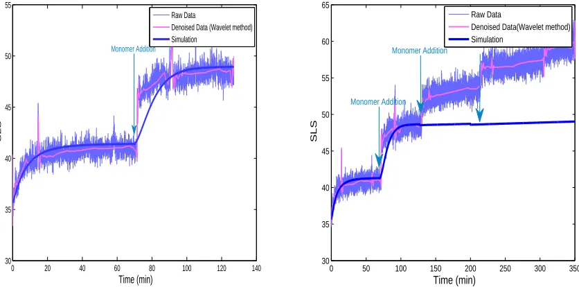
To fit the second addition of monomers, we tested all the previously found sets of kinetic constants (kon, kmon,

kdepand kmdep) that closely mimicked the first addition of monomers. After adjusting these values for a

0 20 40 60 80 100 120 140 30

35 40 45 50 55

Time (min)

SLS

Raw Data

Denoised Data (Wavelet method) Simulation

Monomer Addition

0 50 100 150 200 250 300 350 30

35 40 45 50 55 60 65

Time (min)

SLS

Raw Data

Denoised Data(Wavelet method) Simulation

Monomer Addition Monomer Addition

Figure 4. _{Curve fitting for two (left panel) and four (right panel) successive additions of}

monomers, with the ”two-compartment model” (using kon = 3.5.108mol.L−1.min−1; kdep =

1.6.103_min−1_{; k}m

on= 1.7.104mol.L−1.min−1 and kmdep= 1.10−6min−1)

0 20 40 60 80 100 120 140

0 1 2 3 4 5 6 7 8x 10

−10

Time (min)

Quantity of polymers (mol.L

−1

)

Classic polymers Defective polymers

+ monomers

Figure 5. _{Quantity of defective fibrils as a function of time for the set of kinetic coeffficients}

able to fit the heights of the two first additions of monomers (i.e. set of values used in Figure 5: kon= 3.5.108mol.L−1.min−1, kdep= 1.6.103min−1, kmon= 1.7.104mol.L−1.min−1 and k

m dep =

the third addition did not make it possible to increase sufficiently the simulated signal can be explained by the low kmdepand the high percentage of modified fibrils (Figure 5). Regarding the slopes, the contribution of the

different biological parameters will be mathematically studied in a future sensitivity problem. This study will enable us, for instance, to confirm (or infirm) that a high ratio kmon

km

dep compared to the ratio

kon

kdep could decrease the slopes (as the formation of defective fibrils prevents a further increase in its size).

This work has shown that the basic model with only one type of fibril could not explain the observed ki-netic behavior of prion fibrils. Therefore, a model with at least two compartments is necessary. Biologically speaking, this could be the result of the occurrence of defective fibrils in addition to classic fibrils. This two-compartment model leads to polymerising constant values, kon, from 4.108 up to 4.1012mol.L−1.min−1. Such

a range of values for polymerising constants (also named in literature as association rate constants, kon,ka or k+) is commonly encountered in other examples of protein-protein associations (aggregation) when fast

poly-merising constants are involved [8]. On the other hand, the depolypoly-merising constant values (kdep from 2.103

up to 2.107_min−1_{) are representative for a very high dissociation rate constant which, although rare, as they}

are usually lower than 1min−1_{, can be encountered for another aggregating protein, tubulin [4]. For a better}

modulation of slopes and heights, an additional assumption could be added to the two-compartment model such as a progressive formation of a defective fibril by more than only one monomer. Recent experimental observations from our collaborating team are indeed in favor of such a complementary hypothesis for explaining the kinetics of prion fibrils.

References

[1] J. M. Ball and J. Carr and O. Penrose,The Becker-D¨oring cluster equations: Basic properties and asymptotic behaviour of

solutions, Commun. Math. Phys., 104: 657-692, 1986

[2] R. Becker and W. D¨oring, Ann. Phys, 416: 719-752, 1935

[3] F.P.Da Costa,Asymptotic behaviour of low density solutions to the generalized Becker-D¨oring equations, NoDEA Nonlinear Differential Equations Appl.,5: 23-37,1998

[4] M. Gardner, B. Charlebois, I. J´anosi, J. Howard, A. Hunt, and D. Odde,Rapid Microtubule Self-Assembly Kinetics, Cell, 146: 582-592, 2011

[5] B. Niethammer.On the Evolution of Large Clusters in the Becker-D¨oring Model, J. Nonlinear Sci., 13:115-122, 2003 [6] M. Polymenidou and D. Cleveland,Prion-like spread of protein aggregates in neurodegeneration, J. Exp. Med., 209 : 889-893,

2012

[7] S. Prigent and D. Martin, C. Sizuin, V. Beringue, A. Igel-Egalon, P. Marchand, G. van der Rest, C. Malosse, M. Adrover, M. van Audenhaege, C. Chapuis, J. Torrent and H. Rezaei,Molecular basis of structural information transference during prion conversion, paper in preparation