F´ed´eration Denis Poisson (Orl´eans-Tours) et E. Tr´elat (UPMC), Editors
QUANTUM WAVEGUIDES WITH CORNERS
Monique Dauge
1, Yvon Lafranche
1and Nicolas Raymond
1Abstract. The simplest modeling of planar quantum waveguides is the Dirichlet eigenproblem for the Laplace operator in unbounded open sets which are uniformly thin in one direction. Here we consider V-shaped guides. Their spectral properties depend essentially on a sole parameter, the opening of the V. The free energy band is a semi-infinite interval bounded from below. As soon as the V is not flat, there are bound states below the free energy band. There are a finite number of them, depending on the opening. This number tends to infinity as the opening tends to 0 (sharply bent V). In this situation, the eigenfunctions concentrate and become self-similar. In contrast, when the opening gets large (almost flat V), the eigenfunctions spread and enjoy a different self-similar structure. We explain all these facts and illustrate them by numerical simulations.
R´esum´e. La mod´elisation la plus simple des guides d’ondes quantiques plans est le probl`eme aux valeurs propres pour le laplacien dans des ouverts non born´es qui sont fins dans une direction. Ici nous consid´erons des guides en forme de V. Leurs propri´et´es spectrales d´ependent essentiellement d’un seul param`etre, l’ouverture du V. La bande d’´energie libre est un intervalle semi-infini born´e inf´erieurement. D`es que le V n’est pas plat, il existe des ´etats li´es sous la bande d’´energie libre. Ils sont en nombre fini, fonction de l’ouverture. Ce nombre tend vers l’infini quand l’ouverture tend vers 0 (V tr`es referm´e). Dans cette situation, les fonctions propres se concentrent et deviennent auto-similaires. `A l’oppos´e, quand l’ouverture est grande (V tr`es aplati), les fonctions propres s’´etalent et jouissent d’une autre structure auto-similaire. Nous expliquons tous ces r´esultats et les illustrons par des exp´eriences num´eriques.
Introduction
A quantum waveguide refer to nanoscale electronic device with a wire or thin surface shape. In the first case, one speaks of a quantum wire. The electronic density is low enough to allow a modeling of the system by a simple one-body Schr¨odinger operator with potential
ψ 7−→ −∆ψ+V ψ in R3.
The structure of the device causes the potential to be very large outside and very small inside the device. As a relevant approximation, we can consider that the potential is zero in the device and infinite outside ; this can be described by a Dirichlet operator
ψ 7−→ −∆ψ in Ω and ψ= 0 on ∂Ω
1
IRMAR (UMR CNRS 6625), Universit´e de Rennes 1, France e-mail:[email protected],
e-mail: [email protected], e-mail: [email protected]
c
EDP Sciences, SMAI 2012
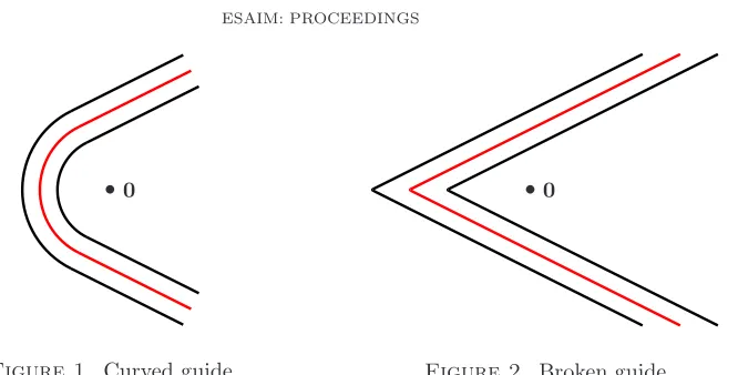
• 0
Figure 1. Curved guide
•0
Figure 2. Broken guide
where Ω is the open set filled by the device. We refer to [3] where we can see, at least on the numerical simulations, the analogy between a problem with a confining potential and a Dirichlet condition.
These kinds of device are intended to drive electronic fluxes. But their shape may capture some bound states, i.e. eigenpairs of the Dirichlet problem:
−∆ψ=λψ in Ω and ψ= 0 on ∂Ω.
The topic of this paper is two-dimensional wire shaped structures,i.e. structures which coincide with strips of the formR+×(0, α) outside a ball of center0and radiusRlarge enough. These structures can be calledplanar
waveguides. More specifically, there are thebent waveguides and thebroken waveguides: Bent waveguides have a constant width around some central smooth curve, see Figure 1, and the central curve of a broken waveguide is a broken line, see Figure 2.
Due to the semi-infinite strips contained in such waveguide, the spectrum of the Laplacian−∆ with Dirichlet conditions is not discrete: It contains a semi-infinite interval of the form [µ,+∞) which is the energy band where electronic transport can occur. The presence of discrete spectrum at lower energy levels is not obvious, but nevertheless, frequent.
A remarkable result by Duclos and Exner [10] (and generalized in [6]) tells us that if the mid-line of a planar waveguide is smooth and straight outside a compact set, then there exists bound states as soon as the line is not straight everywhere. For broken guides, a similar result holds, [2, 11]: There exist bound states as soon as the guide is not a straight strip. The question of the increasing number of such bound states for sharply bent broken waveguides has been answered in [5].
Before stating the main results of this paper, let us mention a few other works involving broken waveguides such as [15, 16]. It also turns out that our analysis leads to the investigation of triangles with a sharp angle as in [14] (see also [4]). The generalization to dimension 3 of the broken strip arises in [12] where a conical waveguide is studied, whereas a Born-Oppenheimer approach is in progress in [28].
and self-similarity appears, which can be explained by a semi-classical analysis: We give some overview of the asymptotic expansions established in our other paper [9]. We end this work by evaluations of the numerical convergence of the algorithms used for our finite element computations (section 9).
Notation. The L2 norm on an open set
U will be denoted byk · kU.
1.
Unbounded self-adjoint operators
In this section we recall from the literature some definitions and fundamental facts on unbounded self-adjoint operators and their spectrum. We quote the standard book of Reed and Simon [30, Chapter VIII] and, for the readers who can read french, the book of L´evy-Bruhl [23] (see in particular Chapter 10 on unbounded operators). Let H be a separable Hilbert space with scalar producth·,·iH. We will consider operatorsA defined on a dense subspaceDom(A) ofH called thedomain ofA. The adjointA∗ofA is the operator defined as follows:
(i) The domainDom(A∗) is the space of the elementsuofH such that the form
Dom(A)∋v7→ hu, AviH
can be extended to a continuous form onH.
(ii) For anyu∈Dom(A∗),A∗uis the unique element ofH provided by the Riesz theorem such that
∀v∈Dom(A), hA∗u, vi
H =hu, AviH (1)
Definition 1.1. The operator Awith domainDom(A) is saidself-adjoint ifA=A∗, which means that Dom(A∗) =Dom(A) and ∀u, v∈Dom(A), hAu, viH =hu, AviH. (2)
1.1.
Operators in variational form
The operators that we will consider can be defined by variational formulation. Let us introduce the general framework first. Let be given two separable Hilbert spacesH and V with continuous embedding ofV intoH and such thatV is dense inH. Letbbe an hermitian sesquilinear form onV
b:V ×V ∋(u, v)7→b(u, v)∈C
which is assumed to be continuous and coercive: This means that there exist three real numbers c, C and Λ such that
∀u∈V, ckuk2
V ≤b(u, u) + Λhu, uiH≤Ckuk2V. (3) LetAbe the operator defined fromV into its dualV′ by the natural expression
∀v∈V, hAu, viH=b(u, v).
In other words, for allu∈V,Auis the linear formv7→b(u, v). Note that the operatorA+ Λ Id is associated in the same way to the sesquilinear form
b+ Λh·,·iH:V ×V ∋(u, v)7→b(u, v) + Λhu, viH ∈C
which is strongly elliptic by (3). As a consequence of the Riesz theorem (or the more general Lax-Milgram theorem) there holds
A+ Λ Id is an isomorphism from V onto V′. (4)
Lemma 1.2. Let A be the operator associated with an hermitian sesquilinear form b coercive on V. LetA be the restriction of the operatorA on the domain
Dom(A) ={u∈V : Au∈H}.
Then A is self-adjoint.
Proof. The operatorAis symmetric becauseb is hermitian. Moreover we check immediately that
∀u, v∈Dom(A), hAu, viH=hu, AviH=b(u, v).
In particular, we deduceDom(A)⊂Dom(A∗). Let us prove thatDom(A∗)⊂Dom(A). Since the domain ofA
andA∗ are unchanged by the addition of Λ Id, and since
(A+ Λ Id)∗=A∗+ Λ Id
we can considerA+ Λ Id instead ofA, or, in other words, using (4), assume thatAis bijective.
Then we deduce thatAis an isomorphism fromDom(A) ontoH: Indeed,Ais injective becauseAis injective; Iff ∈H, there existsu∈V such thatAu=f, andu∈Dom(A) by definition ofDom(A).
Letwbelong toDom(A∗). This means,cf. (2), thatw∈H andA∗w=f ∈H. Let us prove thatwbelongs
toDom(A).
SinceAis bijective there existsu∈Dom(A) such thatAu=f. We have
∀v∈V, b(u, v) =hf, viH
and therefore
∀v∈Dom(A), hu, AviH =hw, AviH.
Hence, asAis bijective, for allg∈H,hu, giH=hw, giH. Finallyu=w, which ends the proof.
Example 1.3. Let Ω be an open set inRn and∂DirΩ a part of its boundary. On
V ={ψ∈H1(Ω) : ψ= 0 on ∂DirΩ}
we consider the bilinear form
b(ψ, ψ′) =
Z
Ω∇
ψ(x)· ∇ψ′(x) dx.
The operatorAis equal to−∆ and it is self-adjoint onH= L2(Ω) with domain
Dom(A) ={ψ∈V : ∆ψ∈L2(Ω) and ∂nψ= 0 on ∂Ω\∂DirΩ}.
1.2.
Discrete and essential spectrum
LetAbe an unbounded self-adjoint operator onH with domainDom(A). We recall the following character-izations of its spectrumσ(A), its essential spectrumσess(A) and its discrete spectrum σdis(A):
• Spectrum: λ∈σ(A) if and only if (A−λId) is not invertible fromDom(A) ontoH,
• Essential spectrum: λ ∈ σess(A) if and only if (A−λId) is not Fredholm1 from Dom(A) into H (see [30, Chapter VI] and [23, Chapter 3]),
• Discrete spectrum: σdis(A) :=σ(A)\σess(A).
We list now several fundamental properties of essential and discrete spectrum.
Lemma 1.4 (Weyl criterion). We haveλ∈σess(A) if and only if there exists a sequence(un)∈Dom(A)such
that kunkH = 1,(un) has no subsequence converging inH and(A−λId)un →
n→+∞0 inH.
From this lemma, one can deduce (see [23, Proposition 2.21 and Proposition 3.11]):
Lemma 1.5. The discrete spectrum is formed by isolated eigenvalues of finite multiplicity.
Lemma 1.6. The essential spectrum is stable under any perturbation which is compact fromDom(A) intoH.
Example 1.7. LetAbe the self-adjoint operator onHassociated with an hermitian sesquilinear formbcoercive onV,cf. Lemma 1.2. Let us assume thatV is compactly embedded inH. Then the spectrum ofAis discrete and formed by a non-decreasing sequence νk of eigenvalues which tend to +∞as k →+∞(see [23, Chapter 13]). Let (vk)k≥1be an associated orthonormal basis of eigenvectors:
Avk =νkvk, ∀k≥1.
Then we have the following identities
∀u∈H, kuk2H =
X
k≥1
u, vk
H
2, (5)
∀u∈V, b(u, u) =X k≥1
νk
u, vkH
2
, (6)
∀u∈Dom(A), kAuk2 H=
X
k≥1 ν2
k
u, vkH
2
. (7)
Example 1.8. Let us define ∆Dir
Ω as the Dirichlet problem for the Laplace operator−∆ on an open set Ω⊂Rn, cf. Example 1.3 with∂DirΩ =∂Ω.
(i)If Ω is bounded, ∆Dir
Ω has a purely discrete spectrum, which is an increasing sequence of positive numbers. (ii) Let us assume that there is a compact setK such that
Ω\K= [
j finite
Ωj (disjoint union)
where Ωj is isometrically affine to a half-tube Σj = (0,+∞)×ωj, withωj bounded open set inRn−1. Letµj be the first eigenvalue of the Dirichlet problem for the Laplace operator−∆ onωj. Then, we have:
σess(∆DirΩ ) =∪j[µj,+∞) = [min
j µj,+∞).
The proof can be organized in two main steps. Firstly, for eachj we construct Weyl sequences supported in Σj associated with anyλ > µj, which proves thatσess(∆ΩDir)⊂[minjµj,+∞). Secondly we apply Lemma 1.6 withA=B−C where A= ∆Dir
Ω andB = ∆DirΩ +W, whereW is a non negative and smooth potential which is compactly supported and such that W ≥ minjµj on K. On one hand, since C is compact, we get that σess(A) =σess(B). On the other hand, we notice that:
Z
Ωk∇
ψk2dx+
Z
Ω
W|ψ|2 dx≥
Z
Ωk∇
ψk2dx+ min j µj
Z
K| ψ|2 dx
and, using the Poincar´e inequality with respect to the transversal variable in each strip Σj:
Z
Ωk∇
ψk2dx≥X
j
Z
Σjk∇
ψk2 dx≥X
j
Z
Σj
µj|ψ|2 dx≥min j µj
Z
We infer that: Z
Ωk∇
ψk2 dx+
Z
Ω
W|ψ|2 dx≥min j µj
Z
Ω| ψ|2 dx.
The min-max principle provides that infσ(B) ≥ minjµj so that infσess(B) ≥ minjµj, and finally we get infσess(A)≥min
j µj.
For an example of this technique, we refer for instance to [6, Section 3.1]. Let us notice that the Persson’s theorem provides a direct proof (see [29] and [13, Appendix B]).
The same formula holds even if the boundary conditions on∂Ω∩K are mixed Dirichlet-Neumann.
1.3.
Rayleigh quotients
We recall now the definition of the Rayleigh quotients of a self-adjoint operatorA(see [23, Proposition 6.17 and 13.1]).
Definition 1.9. The Rayleigh quotients associated to the self-adjoint operatorAonH of domainDom(A) are defined for all positive natural numberj by
λj= inf
u1,...,uj∈Dom(A) independent
sup u∈[u1,...,uj]
hAu, uiH hu, uiH .
Here [u1, . . . , uj] denotes the subspace generated by thej independent vectorsu1, . . . , uj. The following statement gives the relation between Rayleigh quotients and eigenvalues.
Theorem 1.10. Let A be a self-adjoint operator of domainDom(A). We assume thatAis semi-bounded from below, i.e., there existsΛ∈Rsuch that
∀u∈Dom(A), hAu, uiH+ Λhu, uiH≥0.
We set γ= minσess(A). Then the Rayleigh quotientsλj ofA form a non-decreasing sequence and there holds (i) If λj < γ, it is an eigenvalue ofA,
(ii) Ifλj ≥γ, thenλj =γ,
(iii) The j-th eigenvalue< γ ofA (if exists) coincides withλj.
Lemma 1.11. LetAbe the self-adjoint operator onH associated with an hermitian sesquilinear formbcoercive onV,cf. Lemma 1.2. Then the Rayleigh quotients ofA are equal to
λj= inf
u1,...,uj∈V
independent
sup u∈[u1,...,uj]
b(u, u) hu, uiH .
Corollary 1.12. LetAandAˆbe the self-adjoint operators onH andHˆ associated with the hermitian sesquilin-ear forms bandˆb coercive onV andVˆ, respectively. We assume that
ˆ
H ⊂H, Vˆ ⊂V, ˆb(u, u)≥b(u, u)∀u∈V .ˆ
Let λj andλˆj be the Rayleigh quotients associated toA andAˆ, respectively. Then
∀j≥1, ˆλj ≥λj.
Example 1.14 (Monotonicity of Dirichlet eigenvalues). Let Ω be an open subset of Rn and Ωb ⊂ Ω. The
extension by 0 fromΩ to Ω realizes a natural embedding of Hb 1
0(Ω) into Hb 10(Ω), and of L2(Ω) into Lb 2(Ω). Then, with obvious notations:
∀j≥1, λj(∆Dir b
Ω )≥λj(∆ Dir Ω ).
Remark 1.15 (Non-monotonicity of Neumann eigenvalues). The Neumann problem consists in takingH1(Ω) as variational space. The argument above does not work because there is no canonical embedding of H1(Ω)b intoH1(Ω). Moreover, the monotonicity with respect to the domain is wrong:
(i)Let us choose Ω bounded and connected, and Ω a subset of Ω with two connected components. Thenb
λ1(∆Neu b
Ω ) =λ2(∆ Neu b
Ω ) = 0 and λ1(∆ Neu
Ω ) = 0, λ2(∆NeuΩ )>0.
(ii) If we take two embedded intervals forΩ and Ω, then explicit calculations show thatb λj(∆Neu b
Ω )≥λj(∆ Neu Ω ). Another nice and non trivial counter-example can be found with the de Gennes operator appearing in the superconductivity theory,cf.[8].
2.
The broken guide
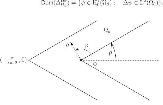
Let us denote the Cartesian coordinates in R2 by x = (x1, x2). The open sets Ω that we consider are
unbounded plane V-shaped sets. The question of interest is the presence and the properties of bound states for the Laplace operator ∆ =∂2
1+∂22 with Dirichlet boundary conditions in such Ω. We can assume without loss of generality that our set Ω is normalized so that
• it has its non-convex corner at the origin0= (0,0), • it is symmetric with respect to thex1 axis,
• its thickness is equal toπ.
The sole remaining parameter is the opening of the V: We denote byθ∈(0,π2) the half-opening and by Ωθthe associated broken guide, see Figure 3. We have
Ωθ=n(x1, x2)∈R2: x1tanθ <|x2|<
x1+ π sinθ
tanθo. (8)
Finally, like in Example 1.8, we specify thepositive Dirichlet Laplacian by the notation ∆Dir
Ωθ. This operator is
an unbounded self-adjoint operator with domain
Dom(∆Dir
Ωθ) ={ψ∈H
1
0(Ωθ) : ∆ψ∈L2(Ωθ)}.
x1 x2
(− π sinθ,0)
Ωθ
ϕ
θ ρ
• 0
The boundary of Ωθ is not smooth, it is polygonal. The presence of the non-convex corner with vertex at the origin is the reason for the domainDom(∆Dir
Ωθ) to be distinct from H
2 ∩H1
0(Ωθ). Nevertheless this domain can be precisely characterized as follows. Let us introduce polar coordinates (ρ, ϕ) centered at the origin, with ϕ= 0 coinciding with the upper part x2 =x1tanθ of the boundary of Ωθ. Let χ be a smooth radial cutoff function with support in the regionx1tanθ <|x2| andχ ≡1 in a neighborhood of the origin. We introduce the explicitsingular function
ψsing(x1, x2) =χ(ρ)ρπ/ωsin πϕ
ω , with ω= 2(π−θ). (9)
Then there holds,cf. the classical references [18, 22]:
Dom(∆Dir Ωθ) = H
2 ∩H1
0(Ωθ)⊕[ψsing] (10)
where [ψsing] denotes the space generated byψsing.
2.1.
Essential spectrum
Proposition 2.1. For any θ∈(0,π2)the essential spectrum of the operator ∆Dir
Ωθ coincides with [1,+∞).
Proof. This proposition is a consequence of Example 1.8(ii): Outside a compact set, Ωθis the union of two strips isometric to (0,+∞)×(0, π). Since the first eigenvalue of−∂2
y on H10(0, π) is 1, the proposition is proved.
2.2.
Symmetry
In our quest of bounded states (λ, ψ) of ∆Dir Ωθ, i.e.
(
−∆ψ=λψ in Ωθ,
ψ= 0 on ∂Ωθ with λ <1, ψ6= 0, (11)
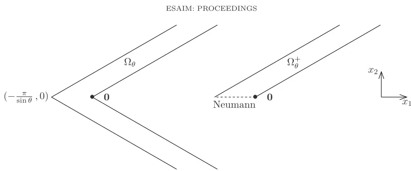
we can reduce to the half-guide Ω+θ defined as (see Figure 4)
Ω+
θ ={(x1, x2)∈Ωθ:x2>0}, with the Dirichlet part of its boundary ∂DirΩ+θ =∂Ωθ∩∂Ω+θ, as we are going to explain now. Let us introduce ∆Mix
Ω+
θ
as the positive Laplacian with mixed Dirichlet-Neumann
conditions on Ω+θ with domain,cf. Example 1.3:
Dom(∆MixΩ+
θ) =
ψ∈H1(Ω+θ) : ∆ψ∈L2(Ω+θ), ψ= 0 on ∂DirΩ+θ and ∂2ψ= 0 on x2= 0 .
Thenσess(∆MixΩ+
θ
) coincides withσess(∆DirΩθ). Concerning the discrete spectrum we have:
Proposition 2.2. For any θ∈(0,π2),σdis(∆DirΩθ)coincides withσdis(∆
Mix Ω+
θ
).
Proof. The proof relies on the fact that ∆Dir
Ωθ commutes with the symmetryS: (x1, x2)7→(x1,−x2).
(i)If (λ, ψ) is an eigenpair of ∆Mix Ω+
θ
, the even extension ofuλ to Ωθ defines an eigenfunction of ∆DirΩθ associated
with the same eigenvalueλ. Therefore we have the inclusion
σdis(∆MixΩ+
θ
)⊂σdis(∆DirΩθ).
(ii)Conversely, let (λ, ψ) be an eigenpair of ∆Dir
Ωθ withλ <1. Splittingψinto its odd and even partsψ
odd and
ψeven with respect tox2, we obtain:
ψ=ψodd+ψeven, ∆Dir Ωθψ
odd=λψodd and ∆Dir Ωθψ
x1 x2
(− π sinθ,0)
Ωθ Ω+θ
Neumann
• 0 • 0
Figure 4. The waveguide Ωθand the half-guide Ω+θ (hereθ= π 6).
We note thatψodd satisfies the Dirichlet condition on the linex
2= 0, andψeventhe Neumann condition on the same line. Let us check thatψodd = 0. If it is not the case, this would mean that λis an eigenvalue for the Dirichlet Laplacian on the half-waveguide Ω+θ. But, by monotonicity of the Dirichlet spectrum with the respect to the domain,cf. Example 1.14, we obtain that the spectrum on Ω+θ is higher than the spectrum on the infinite strip which coincides with Ω+θ whenx1 >0. This latter spectrum is equal to [1,+∞). Therefore the Dirichlet Laplacian on the half-waveguide Ω+θ cannot have an eigenvalue below 1. Thus, we have necessarily: ψodd = 0 andψ=ψevenwhich is an eigenfunction of ∆Mix
Ω+
θ
associated withλ.
We take advantage of Proposition 2.2 for further proofs and for numerical simulations.
3.
Monotonicity of Rayleigh quotients with respect to the opening
From now on we consider the Rayleigh quotients associated with the operator ∆Mix Ω+
θ
, which we write in the form,cf. Lemma 1.11
λj(θ) = inf
ψ1,...,ψj independent inH1(Ω+θ),
ψ1,...,ψj=0on ∂DirΩ+θ
sup ψ∈[ψ1,...,ψj]
k∇ψk2 Ω+
θ
kψk2 Ω+
θ
. (12)
Thoseλj(θ) which are<1 are all the eigenvalues of ∆Dir
Ωθ sitting below its essential spectrum.
Proposition 3.1. For any integerj ≥1, the function θ7→λj(θ) defined in (12)is non-decreasing from(0,π2) intoR+.
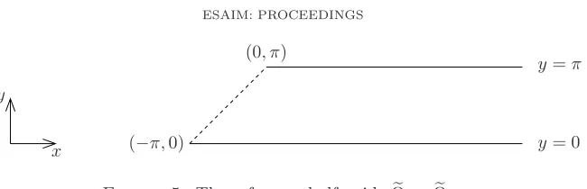
Proof. We cannot use directly Corollary 1.12 because of the part of the boundary where Neumann conditions are prescribed. Instead we introduce the open setΩθe isometric to Ω+θ, see Figure 5,
e
Ωθ=n(˜x,˜y)∈− π tanθ,+∞
×(0, π) : y <˜ x˜tanθ+π if ˜x∈− π tanθ,0
o .
The part ∂DirΩθe of the boundary carrying the Dirichlet condition is the union of its horizontal parts. The numbersλj(θ) can be equivalently defined by the Rayleigh quotients (12) onΩθ.e
Let us now perform the change of variable:
y= 0 y=π (0, π)
(−π,0) x
y
Figure 5. The reference half-guideΩ :=e Ωπ/4.e
so that the new integration domain Ω :=e Ωπ/4e is independent of θ. The bilinear gradient form b on Ωθe is transformed into the anisotropic formbθ on the fixed setΩ:e
bθ(ψ, ψ′) =
Z
e
Ω
tan2θ(∂xψ ∂xψ′) + (∂yψ ∂yψ′) dxdy, (13)
with associated form domain
V :={ψ∈H1(Ω) :e ψ= 0 on∂DirΩe} (14)
independent ofθ.
The functionθ7→tan2θbeing increasing on (0,π
2), we have
∀ψ∈V, θ7→bθ(ψ, ψ) non-decreasing on (0,π 2).
We conclude thanks to Corollary 1.12.
Remark 3.2. Using the perturbation theory, we also know that, for all j ≥ 1, the function θ 7→ λj(θ) is continuous with respect toθ∈ 0,π
2
. Moreover,λ1being simple (as the first eigenvalue of a Laplace-Dirichlet problem), it is analytic because we are in the situation of an analytic family of type (B) (see [21, p. 387 and 395]). In fact the numerical simulations lead to think that all the eigenvalues below 1 are simple and thus analytic.
4.
Existence of discrete spectrum
We recall that the lower bound of the essential spectrum of the operator ∆Mix Ω+
θ
is 1. Its first Rayleigh quotient is given by,cf. (12),
λ1(θ) = inf
ψ∈H1(Ω+
θ), ψ=0 on∂DirΩ+θ
k∇ψk2 Ω+
θ
kψk2 Ω+
θ
. (15)
In this section, we prove the following proposition:
Proposition 4.1. For any θ∈(0,π2), the first Rayleigh quotient λ1(θ) is<1. This statement implies that λ1(θ) is an eigenvalue of ∆Mix
Ω+
θ
(application of Theorem 1.10), hence of the Dirichlet Laplacian ∆Dir
Ωθ on the broken guide (Proposition 2.2).
This statement was first established in [2]. Here we present a distinct, more synthetic proof, using the method of [6, p. 104-105].
Proof. For convenience, it is easier to work in the reference set Ω =e Ωπ/4e introduced in the previous section, with the bilinear formbθ (13) and the form domainV (14). We are going to work with the shifted bilinear form
˜bθ(ψ, ψ′) =bθ(ψ, ψ′)−Z e
Ω
which is associated with the quadratic form:
e
Qθ(ψ) = ˜bθ(ψ, ψ).
Then the first Rayleigh quotient ofQeθis equal toλ1(θ)−1. To prove our statement, this is enough to construct a functionψ∈V such that:
e
Qθ(ψ)<0. This will be done by the construction of
(1) A sequenceψn∈V such thatQeθ(ψn)→0 asn→ ∞,
(2) An elementφofV such that ˜bθ(ψn, φ) is nonzero and independent ofn.
The desired function will then be obtained as a suitable combinationψn+εφ. Let us give details now. Step 1. In order to do that, we consider the Weyl sequence defined as follows. Let χ be a smooth cutoff function equal to 1 forx≤0 and 0 forx≥1. We let, forn∈N\ {0}:
χn(x) =χx n
and ψn(x, y) =χn(x) siny.
Using the support ofχn, we find thatQeθ(ψn) is equal to
Z 0
−π
Z x+π
0
(cos2y−sin2y) dydx+
Z ∞
0
Z π
0
tan2θ(χ′n)2(x) sin2y+χ2n(x)(cos2y−sin2y)
dydx.
Then, elementary computations provide:
Z π
0
(cos2y−sin2y) dy= 0 and
Z 0
−π
Z x+π
0
(cos2y−sin2y) dydx= 0.
Moreover, we have: Z
∞
0
Z π
0
tan2θ(χ′n)2sin2ydydx≤
Z 1
0 |
χ′(u)|2du
πtan2θ
2n . Hence we have proved thatQeθ(ψn) tends to 0 asn→ ∞:
e
Qθ(ψn)≤Kθ
2n with Kθ=
Z 1
0 |
χ′(u)|2du
πtan2θ . (16)
Step 2. We introduce a smooth cutoff function η of x supported in (−π,0). We consider a function f of y∈[0, π] to be determined later and satisfyingf(0) = 0. We defineφ(x, y) =η(x)f(y). Forε >0 to be chosen small enough, we introduce:
ψn,ε(x, y) =ψn(x, y) +εφ(x, y). We have:
e
Qθ(ψn,ε) =Qeθ(ψn) + 2ε˜bθ(ψn, φ) +ε2Qeθ(φ). Let us compute ˜bθ(ψn, φ). We can write, thanks to considerations of support:
˜
bθ(ψn, φ) =
Z 0
−π
Z x+π
0
η(x) cosyf′(y)−sinyf(y)dydx=
Z 0
−π
Z x+π
0
η(x) cosyf(y)′dydx.
Usingf(0) = 0, this leads to:
˜
bθ(ψn, φ) =
Z 0
−π
We choosef(y) =η(y−π) cos(y−π) and we find:
˜
bθ(ψn, φ) =−
Z 0
−π
η2(x) cos2(x) dx=
−Γ<0.
This implies, using (16):
e
Qθ(ψn,ε)≤ Kθ
2n −2Γε+Dε 2,
whereD=Qeθ(φ) is independent ofεandn. There existsε >0 such that:
−2Γε+Dε2≤ −Γε.
The angleθbeing fixed, we can takeN large enough so that
Kθ 2N ≤
Γ 2 ε,
from which we deduce thatQeθ(ψN,ε)≤ −εΓ/2<0, which ends the proof of Proposition 4.1.
5.
Finite number of eigenvalues below the essential spectrum
For a self-adjoint operatorA and a chosen real numberλ we denote byN(A, λ) the maximal indexj such that thej-th Rayleigh quotient ofAis< λ. By extension of notation, if the operatorAis defined by a coercive hermitian formbon a form domainV, and if Qdenotes the associated quadratic formQ(u) =b(u, u), we also denote byN(Q, λ) the numberN(A, λ). This is coherent with the fact that in this case the Rayleigh quotients can be defined directly byQ,cf. Lemma 1.11:
λj = inf
u1,...,uj∈V independent
sup u∈[u1,...,uj]
Q(u) hu, uiH.
This section is devoted to the proof of the following proposition:
Proposition 5.1. For any θ∈(0,π2),N(∆Dir
Ωθ,1)is finite.
Thus in any case ∆Dir
Ωθ has a nonzero finite number of eigenvalues under its essential spectrum.
Proof. For the proof of Proposition 5.1 we use a similar method as [27, Theorem 2.1].
Like for the proof of Proposition 4.1, it is easier to work in the reference setΩ introduced in section 3, withe the bilinear formbθ(13) and the form domain V (14). The opening θbeing fixed, we drop the index θin the notation of quadratic forms and write simply asQthe quadratic form associated withbθ:
Q(ψ) =bθ(ψ, ψ) =
Z
e
Ω
tan2θ|∂xφ|2+|∂yφ|2dxdy.
We recall that the form domainV is the subspace ofψ∈H1(Ω) which satisfy the Dirichlet condition one ∂ DirΩ.e We want to prove that
N(Q,1) is finite. We consider a C1 partition of unity (χ
0, χ1) such that
withχ0(x) = 1 for x <1 andχ0(x) = 0 forx >2. ForR >0 andℓ∈ {0,1}, we introduce:
χℓ,R(x) =χℓ(R−1x).
Thanks to the IMS formula (see for instance [7]), we can split the quadratic form as:
Q(ψ) =Q(χ0,Rψ) +Q(χ1,Rψ)− kχ′0,Rψk2Ωe− kχ′1,Rψk
2
e
Ω. (17)
We can write
|χ′0,R(x)|2+|χ′1,R(x)|2=R−2WR(x) with WR(x) =|χ′0(R−1x)|2+|χ′1(R−1x)|2.
Then
kχ′0,Rψk2Ωe+kχ′1,Rψk
2
e
Ω=
Z
e
Ω
R−2WR(x)|ψ|2dxdy
=
Z
e
Ω
R−2WR(x)
|χ0,Rψ|2+|χ1,Rψ|2dxdy. (18)
Let us introduce the subsets ofΩ:e
O0,R={(x, y)∈Ω :e x <2R} and O1,R={(x, y)∈Ω :e x > R}
and the associated form domains
V0=
n
φ∈H1(O0,R) : φ= 0 on ∂DirΩe∩∂O0,R and on {2R} ×(0, π)
o
V1= H10(O1,R).
We define the two quadratic formsQ0,RandQ1,Rby
Qℓ,R(φ) =
Z
Oℓ,R
tan2θ|∂xφ|2+|∂yφ|2−R−2WR(x)|φ|2dxdy for ψ∈Vℓ, ℓ= 0,1. (19)
As a consequence of (17) and (18) we find
Q(ψ) =Q0,R(χ0,Rψ) +Q1,R(χ1,Rψ) ∀ψ∈V. (20)
Let us prove
Lemma 5.2. We have:
N(Q,1)≤ N(Q0,R,1) +N(Q1,R,1). Proof. We recall the formula for thej-th Rayleigh quotient ofQ:
λj = inf E⊂V dimE=j
sup ψ∈E
Q(ψ) kψk2
e
Ω .
The idea is now to give a lower bound forλj. Let us introduce:
J :
V → V0×V1
As (χ0,R, χ1,R) is a partition of the unity,J is injective. In particular, we notice thatJ :V → J(V) is bijective so that we have:
λj= inf F⊂J(V) dimF=j
sup ψ∈J−1
(F) Q(ψ) kψk2
e
Ω
= inf
F⊂J(V) dimF=j
sup ψ∈J−1
(F)
Q0,R(χ0,Rψ) +Q1,R(χ1,Rψ) kχ0,Rψk2Ωe+kχ1,Rψk2Ωe
= inf
F⊂J(V) dimF=j
sup (ψ0,ψ1)∈F
Q0,R(ψ0) +Q1,R(ψ1) kψ0k2O0,R+kψ1k
2
O1,R
.
AsJ(V)⊂V0×V1, we deduce by an application of Corollary 1.12:
λj ≥ inf F⊂V0×V1
dimF=j
sup (ψ0,ψ1)∈F
Q0,R(ψ0) +Q1,R(ψ1) kψ0k2O0,R+kψ1k2O1,R
=:νj, (21)
LetAℓ,Rbe the self-adjoint operator with domainDom(Aℓ,R) associated with the coercive bilinear form corre-sponding to the quadratic formQℓ,RonVℓ. We see thatνj in (21) is thej-th Rayleigh quotient of the diagonal self-adjoint operatorAR
A0,R 0
0 A1,R
with domain Dom(A0,R)×Dom(A1,R).
The Rayleigh quotients of Aℓ,R are associated with the quadratic formQℓ,R for ℓ= 0,1. Thusνj is the j-th element of the ordered set
{λk(Q0,R), k≥1} ∪ {λk(Q1,R), k≥1}.
Lemma 5.2 follows.
The operatorA0,R is elliptic on a bounded open set, hence has a compact resolvent. Therefore we get:
Lemma 5.3. For all R >0,N(Q0,R,1) is finite.
To achieve the proof of Proposition 5.1, it remains to establish the following lemma:
Lemma 5.4. There existsR0>0 such that, for R≥R0,N(Q1,R,1) is finite. Proof. For allφ∈V1, we write:
φ= Π0φ+ Π1φ, where
Π0φ(x, y) = Φ(x) siny with Φ(x) =
Z π
0
φ(x, y) sinydy (22)
is the projection on the first eigenvector of−∂2
y on H10(0, π), and Π1= Id−Π0. We have, for allε >0:
Q1,R(φ) =Q1,R(Π0φ) +Q1,R(Π1φ)−2
Z
O1,R
R−2WR(x)Π0φΠ1φdxdy
≥Q1,R(Π0φ) +Q1,R(Π1φ)−ε−1 Z
O1,R
R−2WR(x)|Π0φ|2dxdy−ε Z
O1,R
R−2WR(x)|Π1φ|2dxdy. (23)
Since the second eigenvalue of−∂2
y on H10(0, π) is 4, we have:
Z
O1,R
|∂yΠ1φ|2dxdy
≥4kΠ1φk2
Denoting byM the maximum ofWR (which is independent ofR), and using (19) we deduce
Q1,R(Π1φ)≥(4−M R−2)kΠ1φk2
O1,R.
Combining this with (23) where we takeε= 1, and with the definition (22) of Π0, we find
Q1,R(φ)≥qR(Φ) + (4−2M R−2) kΠ1φk2
O1,R,
where
qR(Φ) =
Z ∞
R
tan2θ|∂xΦ|2+ |Φ|2
−R−2WR(x)|Φ|2dx
≥
Z ∞
R tan2θ
|∂xΦ|2+ |Φ|2
−R−2M
1[R,2R]|Φ|2dx.
We chooseR=√M so that (4−2M R−2) = 2, and then
Q1,R(φ)≥q˜R(Φ) + 2kΠ1φk2
O1,R, (24)
where now
˜ qR(Φ) =
Z ∞
R tan2θ
|∂xΦ|2+ (1
−1[R,2R])|Φ|2dx. (25)
Let ˜aR denote the 1D operator associated with the quadratic form ˜qR. From (24)-(25), we deduce that thej-th Rayleigh quotient ofA1,Radmits as lower bound the j-th Rayleigh quotient of the diagonal operator:
˜
aR 0
0 2 Id
so that we find:
N(Q1,R,1)≤ N(˜qR,1).
Finally, the eigenvalues<1 of ˜aRcan be computed explicitly and this is an elementary exercise to deduce that
N(˜qR,1) is finite.
This concludes the proof of Proposition 5.1.
6.
Decay of eigenvectors at infinity – Computations for large angles
6.1.
Decay at infinity
In order to study theoretical properties of eigenvectors of the operator ∆Dir
Ωθ corresponding to eigenvalues
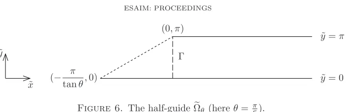
below 1, we use the equivalent configuration on Ωθe introduced in section 3, see also Figure 6. The eigenvalues <1 of ∆Dir
Ωθ are the same as those of ∆
Mix e
Ωθ (with Dirichlet conditions on the horizontal parts of the boundary of
e
Ωθ) and the eigenvectors are isometric. The main result of this section is a quasi-optimal decay in the straight part (0,+∞)×(0, π) of the setΩθe as x→ ∞.
Proposition 6.1. Let θ∈(0,π
2). Letψ be an eigenvector of ∆MixΩeθ associated with an eigenvalue λ <1. Then
for allε >0 the following integral is finite:
Z ∞
0
Z π
0
e2˜x(√1−λ−ε) |ψ(˜x,y˜)|2+
|∇ψ(˜x,y˜)|2d˜yd˜x <
˜ y= 0 ˜ y=π (0, π)
(−tanπθ,0) ˜
x ˜
y Γ
Figure 6. The half-guideΩθe (hereθ= π6).
Proof. We give here an elementary proof based on the representation ofψas solution of the Dirichlet problem in the half-strip Σ :=R+×(0, π)
−∆ψ=λψ in Σ,
ψ(˜x,0) = 0, ψ(˜x, π) = 0 ∀x >˜ 0, ψ(0,y˜) =g ∀y˜∈(0, π)
(27)
where g is the trace of ψ on the segment Γ, see Figure 6. Since ψ belongs to H1(Σ), its trace on∂Σ belongs to H1/2. Because of the zero trace on the lines ˜y = 0 and ˜y =π, we find thatg belongs to the smaller space2 H1/200 (Γ), which is the interpolation space of index 1
2 between H 1
0(Γ) and L2(Γ),cf.[24]. We expand ψ on the eigenvector basis of the operator −∂2
y, self-adjoint on H2∩H10(0, π). Its normalized eigenvectors are
vk(˜y) =
r
2
π sinky˜ with eigenvalue νk=k 2.
We expandgin this basis:
g(˜y) =X k≥1
gkvk(˜y), where gk=
Z π
0
g(˜y)vk(˜y) d˜y.
Interpolating between (5) and (6), we find
kgk2
H100/2(Γ)≃
X
k≥1 k g2k.
We can easily solve (27) by separation of variables. We find
ψ(˜x,y˜) =X k≥1
e−x˜√k2−λ
gkvk(˜y). (28)
The estimate ofψin (26) is then trivial. Let us prove now the estimate of∂x˜ψ. We use thatPk≥1k gk2is finite so that we can write:
∂x˜ψ(˜x,y˜) =−
X
k≥1
p
k2−λe−x˜√k2−λ
gkvk(˜y).
We have:
ex(˜√1−λ−ε)∂x˜ψ(˜x,y˜) =−
X
k≥1
p
k2−λex˜(√1−λ−√k2−λ ) e−ε˜xg
kvk(˜y)
2The space H1/2
00 (Γ) is the subspace of H 1/2
(Γ) spanned by the functionsvsuch that Zπ
0 v2
(˜y) ˜
leading to the L2 estimate:
Z ∞
0
Z π
0
ex(˜√1−λ−ε)∂x˜ψ(˜x,y˜)
2d˜yd˜x=X k≥1
Z ∞
0
(k2−λ) e2˜x(√1−λ−√k2−λ) e−2ε˜xgk2d˜x
≤ X
k≥1 k g2k
sup k≥1
Z ∞
0
ke−2γ˜x√k2−1 e−2ε˜xd˜x,
where γ=γ(λ)>0 is a constant, uniform with respect to k≥1. Using the change of variables ˜x7→√kx˜, we can see that the integrals
Z +∞
0
ke−2˜x(ε+γ√k2−1)
are uniformly bounded ask→ ∞, which ends the proof of the estimate of∂x˜ψin (26). The estimate of∂y˜ψis
similar.
Remark 6.2. Under the conditions of Proposition 6.1, we have also a sharp global L∞ estimate
ke˜x√1−λψkL∞
(eΩθ)<∞.
To prove this we use again the representation (28) and the fact that the traceg is more regular than H1/200 (Γ). In fact, as a consequence of the characterization (10) of the domain of the operator ∆Dir
Ωθ, the tracegbelongs to
H1
0(Γ) and, therefore, the sum
P
k≥1k2g2k is finite by (6). Then, we have:
ex˜√1−λψ(˜x,y˜) =X k≥1
ex˜(√1−λ−√k2−λ)gkvk(˜y).
Taking absolute values, we get:
ex˜√1−λ|ψ(˜x,y˜)| ≤
r
2 π
X
k≥1 |gk| ≤
r
2 π
X
k≥1
k−21/2 X k≥1
k2|gk|2
1/2 .
Remark 6.3. The estimate (26) can also be proved with a general method due to Agmon (see for instance [1]).
6.2.
Computations for large angles
Whenθ→ π
2,λ1(θ) tends to 1, see [2]. The representation (28) shows that in such a situation, the behavior of the associated eigenvectorψis dominated by its first term, proportional to
e−x˜√1−λ sin(˜y).
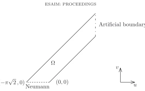
In order to compute such an eigenpair by a finite element method, we have to be careful and take large enough domains — we simply put Dirichlet conditions on an artificial boundary far enough from the corners of the guide. Our computations are performed in the model half-guide Ω := Ω+π/4for the scaled operator
Lθ:=−2 sin2θ ∂2
u−2 cos2θ ∂v2 (29)
equivalent to−∆ in Ω+θ through the variable change
u=x1 √
2 sinθ and v=x2 √
u v
(0,0) (−π√2,0)
Ω
Neumann
Artificial boundary
Figure 7. The model half-guide Ω := Ω+π/4.
We use a Galerkin discretization by finite elements in a truncated subset of Ω with Dirichlet condition on the artificial boundary, see Figure 7. According to Corollary 1.12,cf. also Examples 1.13 and 1.14, the eigenvalues λcptj (θ) of the discretized problem are larger than the Rayleigh quotients λj(θ) ofLθ. When the discretization gets finer and the computational domain, larger,λcptj (θ) tends toλj(θ) forj= 1,2, . . .
For the values ofθconsidered in this section (θ≥ π
4), the numerical evidence is that the discrete spectrum of
Lθ has only one elementλ1(θ). The numerical effect of this is the convergence to 1 of all other computational
eigenvaluesλcptj (θ) forj = 2,3, . . .
The computations represented in Figure 8 are performed with the artificial boundary set at the abscissa u = 5π√2. The plots are mapped back to the corresponding physical domain by a postprocessing of the numerical results.
The computations in Figure 9 are performed with the artificial boundary set at the abscissau= 10π√2. The plots use the computational domain because the corresponding physical domains would be too much elongated to be represented.
7.
Accumulation of eigenpairs for small angles
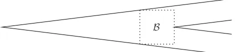
Whenθtends to 0, there is more and more room for eigenvectors between the two corners of the guide. For any rectangular box B contained in Ωθ like in Figure 10, by the monotonicity of Dirichlet eigenvalues (Example 1.13), we know that for anyj
λj(θ)≤λj(B)
where λj(θ) are the Rayleigh quotients of ∆DirΩθ and λj(B) the Dirichlet eigenvalues onB. We choose Bin the
form of a rectangle bounded by the vertical linesx1 =−απ and x1 = 0, and the horizontal lines x2 =±βπ. Thusαandβ satisfy,cf. (8)
α∈(0, 1
sinθ), βπ= (−αsinθ+ 1) π cosθ.
The eigenvalues of the Dirichlet problem inBare
k2 4β2 +
ℓ2
θ= 0.5000∗π/2 λcpt1 (θ) = 0.92934
θ= 0.5983∗π/2 λcpt1 (θ) = 0.96897
θ= 0.6889∗π/2 λcpt1 (θ) = 0.98844
Figure 8. Computations for moderately large angles. Plots of the first eigenvectors in the physical domain (rotated by π
2). Numerical value of the corresponding eigenvalueλ1(θ).
We look for the eigenvaluesλj(B) less than 1. Thereforeαhas to be chosen>1. Thusβ <(1−sinθ)/cosθ≤1 for anyθ. As a consequencek= 1 and the eigenvaluesλj(B) less than 1 are necessarily of the form
λj(B) = 1 4β2 +
j2 α2
= cos
2θ 4(1−αsinθ)2 +
j2 α2.
We optimizeB: The minimum ofλj(B) is obtained forαsuch that
sinθcos2θ 2(1−αsinθ)3 −
θ= 0.7022∗π/2 θ= 0.8538∗π/2 θ= 0.9702∗π/2 λcpt1 (θ) = 0.9903037 λcpt1 (θ) = 0.9994215 λcpt1 (θ) = 0.9999998
Figure 9. Computations for very large angles with the mesh M4L (see Figure 17). Plots in the computational domain Ω.
x1 x2
B
Figure 10. The waveguide Ωθand a Dirichlet boxBinside.
Since we are interested in the behavior asθ→0, we take without asymptotic loss
α= 41/3j2/3sin−1/3θ
which provides
λj(B) = 1 4
cos2θ
(1−41/3j2/3sin2/3θ)2 + 4
1/3j2/3sin2/3θ.
As a consequence, as soon as the quantityZ:= 41/3j2/3sin2/3θ is less that the first root of the equation
1 4
1
(1−Z)2 +Z
= 1,
i.e. for Z ≤0.4679, we haveλj(B)<1 and, hence, λj(θ)<1. This implies that the maximal numberJ such thatλJ(B)<1 is greater than
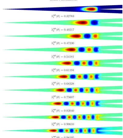
0.46793/2·0.5 sin−1θ≃0.1601 sin−1θ . Therefore the number of eigenvalues of ∆Dir
Ωθ less than 1 tends to infinity (at least) likeθ
−1as θtends to 0. We present in Figure 11 the computations of the all eigenpairs of ∆Dir
Ωθ for the angle θ= 0.0226∗π/2. We
λcpt1 (θ) = 0.32783
λcpt2 (θ) = 0.40217
λcpt3 (θ) = 0.47230
λcpt4 (θ) = 0.54181
λcpt5 (θ) = 0.61194
λcpt6 (θ) = 0.68328
λcpt7 (θ) = 0.75607
λcpt8 (θ) = 0.83040
λcpt9 (θ) = 0.90610
λcpt10(θ) = 0.98195
Figure 11. Computations for θ = 0.0226∗π/2 ∼ 2◦ with the mesh M64S (see Figure 18).
Numerical values of the 10 eigenvaluesλj(θ) <1. Plots of the associated eigenvectors in the physical domain.
8.
Asymptotic behavior of eigenpairs for small angles
We present in Figures 12 and 13 computations of the first eigenvector for smaller and smaller values of the angle θ. We notice that the eigenvectors look similar, with the appearance of a short scale in the horizontal variable.
θ= 0.1482∗π/2 θ= 0.1032∗π/2 θ= 0.0701∗π/2 λcpt1 (θ) = 0.56209 λcpt1 (θ) = 0.48754 λcpt1 (θ) = 0.42763
Figure 12. Computations for small angles. Plots in the computational domain Ω.
θ= 0.0416∗π/2 θ= 0.0270∗π/2 θ= 0.0112∗π/2
λcpt1 (θ) = 0.37085 λ cpt
1 (θ) = 0.33845 λ
cpt
1 (θ) = 0.29766
Figure 13. Computations for very small angles. Plots in the computational domain Ω.
Let us recall that the eigenvaluesλj(θ)<1 of our operator ∆Dir
Ωθ coincide with those of the scaled operator
Lθ:=−2 sin2θ ∂2u−2 cos2θ ∂v2
in the model half-guide Ω. The construction and validation of asymptotic expansions for the eigenpairs ofLθ
rely on a Born-Oppenheimer approximation. Roughly, this consists of four steps: (1) Definition of an operator LBO
θ in the horizontal variableu by replacing the operator in the vertical variableNu:=−2 cos2θ ∂2
v in each slice u= const. by its first eigenvalue Λ(u) (2) Semi-classical analysis of the eigenpairs ofLBO
θ as θ→0.
(3) Determination of a change of variables (u, v)7→(u, t) on Ω in order to exhibit a tensor product structure. Here appears the role of the limit operatorN0− asuր0. Its first eigenvector isv7→cos(v/2).
−50 0 5 0.5
1 1.5 2 2.5
Function Λ Function V
Figure 14. The Born-Oppenheimer potential Λ and its left tangent at u= 0 (here cos2θ is set to 1).
Step 1: Definition ofLBO θ .
LetI(u) be the intersection of Ω with the vertical line of abscissau.
• Foru∈(−π√2,0), I(u) = (0, u+π√2). The operatorNu has Neumann condition at 0 and Dirichlet
atu+π√2. Thus
Λ(u) = 2 cos2θ π 2
4(u+π√2)2
• Foru∈(0,+∞),I(u) = (u, u+π√2). The operatorNu has Dirichlet conditions at both ends. Thus
Λ(u) = cos2θ.
The Born-Oppenheimer operator is
LθBO=−2 sin2θ ∂2u+ Λ(u).
Step 2: Semi-classical analysis ofLBO θ . The operatorLBO
θ can be viewed as a 1D Schr¨odinger operator with potential Λ. The potential has a well with bottom atu= 0. The well is not smooth and has a triangular shape, see Figure 14.
The behavior of the eigenpairs ofLBO
θ asθ →0 is governed by the Taylor expansion of the potential Λ at the well bottomu= 0,i.e. by the tangent potentialV defined by
V(u) = cos2θ
1 4 −
u
2π√2, ifu <0,
1, ifu >0.
The corresponding model problem is the problem of the behavior ash→0 of the eigenpairs of the operator
Hh=−h2∂2
u+
(
The potential barrier on (0,+∞) produces a Dirichlet condition atu= 0 for the leading terms of the asymptotics: We are led to the Airy-type eigenvalue problem
−h2∂u2ψh−uψh=Ehψh on (−∞,0), with ψ(0) = 0. (30)
The change of variablesu7→X =uh−2/3 transforms the above equation into the reverse Airy equation
−∂2XΨ−XΨ =µΨ on (0,+∞), with Ψ(0) = 0, (whereµ=h−2/3Eh)
whose solutions can be easily exhibited: As we will see, the eigenvalues µ are the zeros of the reverse Airy functionA(X) :=Ai(−X), whereAi is the standard Airy function. The zeros ofAform an increasing sequence of positive numbers, which we denote byzA(j),j ≥1.
Since−A′′(X)−XA(X) = 0 we have for anyE∈R
−A′′(X)−(X−E)A(X) =EA(X) i.e. −A′′(X+E)−XA(X+E) =EA(X+E).
IfE=zA(j), thenA(X+E) vanishes atX = 0, hence
zA(j),A X+zA(j)
is an eigenpair.
Conversely, all eigenpairs are of this form.
We deduce that the eigenvalues of problem (30) are Eh = h2/3zA(j) and the associated eigenvectors are ψ(u) =A(uh−2/3+z
A(j)).
Coming back to our operatorLBO
θ , we prove in [9] that its eigenvalues have asymptotic expansions of the form
λBOj (θ) ≃ θ→0
1 4+
2θ2/3zA(j) (4π√2)2/3 +
X
n≥3
θn/3γj,nBO, (31)
whereγBO
j,n are some real coefficients. The eigenvectors have expansions in powers ofθ1/3, using the scaleuh−2/3 foru <0 anduh−1foru >0.
Step 3: Tensorial structure ofLθ.
On the left part of Ω,i.e. its triangular part Triin the half-planeu <0, we perform a change of variables to transformTriinto a square:
Tri∋(u, v)7→(u, t)∈(−π√2,0)×(0, π√2), with t= v π √
2
u+π√2. (32)
On the right part of Ω,i.e. its strip part contained in the half-planeu >0, we perform a change of variables to transform it into a horizontal strip:
(u, v)7→(u, τ)∈(0,+∞)×(0, π√2), with τ=v−u. (33)
This allows to work with the Taylor expansions of the transformed operator aroundu= 0, on the left and on the right. The operator N0− =−2∂t2 appears on the left with Dirichlet condition at t = 1 and Neumann at t= 0. Its first eigenvector is cost
2, associated with the eigenvalue 1
4. The operatorN0+=−2∂ 2
τ appears on the right with Dirichlet condition att= 0,1.
Step 4: Asymptotics of the eigenpairs ofLθ.
The projection on the eigenvectort7→cost
2 appears naturally at the first step of the expansion (this projection is sometimes called Feshbach or Grushin projection) and lets appearLBO
u v
u τ
u t
Tri Ω
Figure 15. The model waveguide Ω and the change of variables.
0 0.1 0.2 0.3 0.4 0.5 0.6 0.7 0.8 0.9 1 0
0.2 0.4 0.6 0.8 1
1st computed eigenvalue 2d computed eigenvalue Essential spectrum
Linear approximation of 1st eigenvalue Linear approximation of 2d eigenvalue
Figure 16. The eigenvaluesλ1 andλ2as functions of (θ∗2/π)2/3.
can be constructed, and in a further step, validated. As a resultλj(θ) has an expansion similar toλBO
j (θ), with different coefficients forn≥3:
λj(θ) ≃ θ→0
1 4 +
2θ2/3z A(j) (4π√2)2/3 +
X
n≥3 θn/3γ
j,n (34)
where γj,n are some real coefficients. In Figure 16 we display the functions (θ∗2/π)2/3 7→ λj(θ) for j = 1,2 (computed by finite elements) and their linear approximation as θ → 0, corresponding to the two-term approximation in (34),i.e. (θ∗2/π)2/3
7→ 1 4+
2θ2/3z
A(j)
(4π√2)2/3.
In the reference domain Ω, the eigenvectors ofLθ have a multiscale expansion in powers ofθ1/3. On the left
is only the ultra-short scale. The asymptotics is dominated by its first term, which is
A u
θ2/3 −zA(1)
cos t 2 .
This structure explains the results seen in Figures 12-13.
9.
Convergence of the finite element method
We now present some aspects of the computation process that led to the numerical results shown in the previous sections.
As described in the section 6.2, the eigenvalue problem writesLθψ=λψ in the domain Ω with homogeneous
Dirichlet conditions on its boundary, except on the horizontal segment where Neumann conditions are set, see identity (29) and Figure 7. The associate bilinear form is
b(ψ, ψ′) =
Z
Ω
2 sin2θ(∂uψ ∂uψ′) + 2 cos2θ(∂vψ ∂vψ′) dudv
defined on the corresponding form domain
V ={ψ∈H1(Ω) : ψ= 0 on∂DirΩ}.
The eigenvalue problem writes in variational form: find non-zeroψ∈V and λsuch that
∀ψ′ ∈V, b(ψ, ψ′) =λψ, ψ′L2(Ω).
By Galerkin projection on a finite dimension subspaceVfdsofV, this problem can be rewritten as the generalized eigenvalue problem: find the eigenpairs (λ, w) such thatSw=λM w, whereSandM are the stiffness and mass matrices associated with a basis (Ψ1, . . . ,ΨN) ofVfds:
S=b(Ψj,Ψk)
1≤j,k≤N and M =
Ψj,ΨkL2(Ω)
1≤j,k≤N.
The computation process consists of two main steps: first, using a finite element method that leads to the two matricesS andM, and second, using an algorithm to compute the eigenpairs. In the following two sections, we focus on the algorithm for the computation of the eigenpairs and then on the influence of the choice of meshes and polynomial degrees in the finite element method.
All the computations have been done in double precision arithmetic, on a iMac computer (4 GB memory, 3.06 GHz Intel Core 2 Duo processor).
9.1.
Computation of the eigenpairs
We have first written a program using the Fortran 77 finite element library “Melina” [25], which also provides a routine to compute eigenpairs of real symmetric eigenvalue problems. This routine uses an algorithm based on subspaces iterations. We callMelthis method.
We have also written another program using the C++ version of the previous library, called “Melina++”. The computation of the eigenpairs have been made using the well-known package ARPACK++ [17]. We call Arpthis method. We thus were able to reproduce the results obtained with the Melmethod, which is a cross validation of both methods.
Here, we compare the computation of the eigenpairs with the two methods. For this purpose, in both cases, we fix the parameters governing the finite element part: interpolation degree 6 at Gauss-Lobatto points, quadrature rule of degree 13.
• “large angle” configuration: θ= 0.9702∗π/2, 4 eigenvalues computed, mesh M4L with 656 triangles (see Figure 17), leading to matrices of size 12325×12325;
• “small angle” configuration: θ= 0.0226∗π/2, 12 eigenvalues computed, mesh M64S with 6144 triangles (see Figure 18), leading to matrices of size 111265×111265.
Although the internal algorithms of the two methods are different, the parameters governing the computation of the eigenvalues are the same: a toleranceεthat controls the end of the iteration process, and the dimension Nsub of the subspaces involved in the subspace iteration — Nsub is at least equal to Nval+ 1, where Nval is the number of desired eigenvalues. We letNsub vary between 10 and 70 and ran the programs for ε= 10−n, n= 4,5,6,7, while recording the number of iterations and the CPU time needed. The CPU time of the finite element part, i.e. the computation of the matricesS andM, does not depend on these parameters. It appears on the graphs asCPUef.
The results are gathered on Figure 19 for the “large angle” configuration and on Figure 20 for the “small angle” configuration. We can observe that the number of iterations decreases as Nsub increases. A horizontal line at the beginning of the first two graphs indicates a failed computation (no convergence after the chosen maximal number of iterations). For the values tested, the parameterεdoes not play a significant role on the number of iterations, nor really on the CPU time (although it does on the residual). Since the algorithms used in the two methods are not the same, the number of iterations cannot be compared directly. They are mainly a good indicator of the computation process behavior.
It is also worth to notice that the memory requirements increase as the subspace dimensionNsubincreases. This parameter is difficult to handle since it is problem dependent. These graphs suggest that there is no critical value: it can be chosen large enough to ensure computation to succeed, but not too large, mainly because of memory considerations.
The CPU graphs of theArpmethod seem a bit chaotic: both algorithms need an initial vector which is chosen as a random vector by default. From our experience, we can say that this method is more sensible to this initial vector than theMelmethod. Finally, these graphs show clearly that theArpmethod is more efficient than the Melmethod.
Remark 9.1. We are interested in the smallest eigenvalues of the problemSw=λM w. Both methodsArpand Melprovide an option to choose in which end of the spectrum the wanted eigenvalues are to be searched. Let us mention that these algorithms perform better at computing the largest eigenvalues in general (this is due to the fact that they are ultimately based on the power method). In our case, this is typical and computation nearly always fails if the algorithms are asked to compute the smallest eigenvalues of this problem. For example, with ARPACK, we can observe the following behavior:
• in the “large angle” configuration, forε= 10−4andN
sub= 17 or 45, the computation fails ; • in the “small angle” configuration, for ε = 10−4 and N
sub = 27 or 43, the computation fails ; if we change the mesh to a coarser one (M16S) with 384 triangles, the computation fails forNsub = 27 and succeeds forNsub= 43 with a CPU time of 236 sec.
Thus, the correct strategy is to compute the largest eigenvalues of the eigenvalue problem M w = νSw and retrieve the wanted eigenvaluesλby inversion (λ= 1/νand the eigenvectors are the same). All the computations presented here have been carried on using this strategy. To conclude this remark, let us mention that the computation that took 236 sec. with the wrong strategy, takes 0.47 sec. with the right one.
9.2.
Influence of meshes and polynomial degrees in the finite element method
We now choose the small angleθ = 0.0226∗π/2 and fix the parameters governing the computation of the eigenvalues: ε= 10−6,N
sub= 25,Nval= 10, since there are 10 eigenvalues<1 as shown on Figure 11.
0 20 40 60 80 100 0
10 20 30 40 50 60 70 80 90
Figure 17. Mesh M4L for large angle, 656 triangles.
−5 −4 −3 −2 −1 0 1
0 1 2 3 4 5
10 20 30 40 50 60 70 0 100 200 300 400 500
Number of iterations
M4L, θ = 0.9702 * π/2, N = 12325, CPUef = 2 s, Arp
1e−04 1e−05 1e−06 1e−07
10 20 30 40 50 60 70
0 10 20 30 40 Subspace dimension
CPU time (sec.)
10 20 30 40 50 60 70
0 400 800 1200
M4L, θ = 0.9702 * π/2, N = 12325, CPUef = 1 s, Mel
1e−04 1e−05 1e−06 1e−07
10 20 30 40 50 60 70
40 60 80 100 120 140 Subspace dimension
Figure 19. Comparison of the behavior of the methods for the large angleθ= 0.9702∗π/2.
10 20 30 40 50 60 70
0 10 20 30
Number of iterations
M64S, θ = 0.0226 * π/2, N = 111265, CPUef = 257 s, Arp
1e−04 1e−05 1e−06 1e−07
10 20 30 40 50 60 70
10 15 20 25
Subspace dimension
CPU time (sec.)
10 20 30 40 50 60 70
0 20 40 60
M64S, θ = 0.0226 * π/2, N = 111265, CPUef = 598 s, Mel
1e−04 1e−05 1e−06 1e−07
10 20 30 40 50 60 70
100 150 200 250
Subspace dimension
Figure 20. Comparison of the behavior of the methods for the small angleθ= 0.0226∗π/2.
diameter h of the triangles, which is halved from a mesh to the next one in the list. Thus, the number of triangles is multiplied by 4 from a mesh to the next one.
We have computed the 10 eigenvalues forε= 10−8using the finest mesh M64S and considered the first and last eigenvalues obtained as reference values. We denote them byλref
1 andλref10.
• with respect to the interpolation degree for a given mesh ; • with respect to the mesh, for a given degree.
The numberN of degrees of freedom (d.o.f.) of the problem, which is the dimension of the matrices, is roughly proportional to (kn)2, which explains the choice of the abscissa log
10(N)/2. The precision attained is about one order of magnitude better for the first eigenvalueλ1 than for the last oneλ10. For the first eigenvalue and the coarser meshes, we observe a kind of super convergence for the small degrees, then a linear convergence. The convergence tends to be linear as the mesh becomes finer. For the last eigenvalueλ10, the convergence is mainly linear.
−5 −4 −3 −2 −1 0 1
0 1 2 3 4 5
−5 −4 −3 −2 −1 0 1
0 1 2 3 4 5
Figure 21. Meshes M4S (24 triangles) and M8S (96 triangles).
−5 −4 −3 −2 −1 0 1
0 1 2 3 4 5
−5 −4 −3 −2 −1 0 1
0 1 2 3 4 5
Figure 22. Meshes M16S (384 triangles) and M32S (1536 triangles).
0.5 1 1.5 2 2.5 −5 −4 −3 −2 −1 0 1 1 2 3 4 5 6 1 2 3 4 5 6 1 2 3 4 5 6 1 2 3 4 5 6 1 2 3 4 5 log
10(Number of d.o.f.)/2
log
10
(|err(
λ
)|)
θ = 0.0226 * π/2 − λ
1 = 0.327833
M4S M8S M16S M32S M64S
0.5 1 1.5 2 2.5
−5 −4 −3 −2 −1 0 1 1 2 3 4 5 6 1 2 3 4 5 6 1 2 3 4 5 6 1 2 3 4 5 6 1 2 3 4 5 log
10(Number of d.o.f.)/2
θ = 0.0226 * π/2 − λ
10 = 0.981955
M4S M8S M16S M32S M64S
Figure 23. Convergence towardsλ1≃0.32783 and λ10≃0.98195.
The average rate of convergence with respect to k−1 is twice the rate of convergence with respect to h, in accordance with a well-known convergence result in finite elements [31]. Typically the rate is 1 in hand 2 in k−1. These somewhat low rates are due to the singularity at the reentrant corner of Ω. This singularity comes from the Laplace singularity (9), and forθ= 0.0226∗π/2, the singularity exponent ωπ is≃0.5057.