Adaptive numerical methods for PDEs

ESAIM: Proceedings, , ,

http://www.emath.fr/Maths/Proc/Vol.11/ c

2002, Soci´et´e de Math´ematiques Appliqu´ees et Industrielles, EDP Sciences

Adaptive numerical methods for PDEs

Ronald A. DeVore

R´esum´e. Les m´ethodes adaptatives sont d’usage courant pour la r´esolution num´erique des EDP. Il n’existe cependant pas de th´eorie bien ´etablie analysant leur performance et jus-tifiant leur utilisation. L’objet de cet expos´e est de pr´esenter les premiers ´el´ements d’une telle th´eorie, dont les pierres angulaires sont l’approximation non-lin´eaire et les th´eor`emes de r´egularit´e pour les EDP. Une m´ethode adaptative num´erique peut ˆetre assimil´ee `a une forme d’approximation non-lin´eaire, la solution de l’´equation n’´etant pas approch ´ee par une suite d’espaces fix´ee `a l’avance, mais par les ´el´ements d’un ensemble non-lin´eaire de fonctions d´ecrit par N param`etres (´el´ements finis adaptatifs, ondelettes). La th´eorie de l’approximation non-lin´eaire relie l’efficacit´e de ce type d’approximation `a la r´egularit´e de la solution mesur´ee dans certains espaces de Besov. L’analyse de cette r´egularit´e pour une ´equation donn´ee d´etermine ainsi le potentiel d’une m´ethode adaptative par comparaison avec les m´ethodes lin´eaires pour lesquelles une th´eorie similaire existe et fait intervenir d’autres classes de r´egularit´e. Une telle approche est illustr´ee dans le cadre elliptique et hyperbolique. Nous pr´esentons finalement un algorithme adaptatif utilisant les ondelettes pour les ´equations el-liptiques d´evelopp´e par Albert Cohen, Wolfgang Dahmen et l’auteur, algorithme dont les performances sont optimales au sens o `u elles refl`etent les taux d’approximation pr´edits par la th´eorie.

Mots cl´es. Equations aux d´eriv´ees partielles, m´ethodes num´eriques, m´ethodes adaptatives, r´egularit´e, vitesse de convergence

Abstract. While adaptive numerical methods are often used in solving partial differential equations, there is not yet a cohesive theory which justifies their use or analyzes their perfor-mance. The purpose of this talk is to put forward the first building blocks of such a theory, the cornerstones of which are nonlinear approximation and regularity theorems for PDEs. Any adaptive numerical method can be viewed as a form of nonlinear approximation: the solution

of the PDE is approximated by elements from a nonlinear manifold of functions. The theory of nonlinear approximation relates the efficiency of this type of approximation to the regular-ity of

in a certain family of Besov spaces. Regularity for PDEs are needed to determine the smoothness of

in this new Besov scale. Together, the approximation theory and regular-ity theory determine the efficiency of approximation that is possible using adaptive methods. A similar analysis gives the efficiency of linear algorithms. The two can then be compared to predict whether nonlinear methods would result in better performance. Examples will be given in the setting of both elliptic and hyperbolic problems. A wavelet based algorithm

1_{This work has been supported in part by the Office of Naval Research Contract N0014-91-J1343 and the Army} Research Office Contract DAAG55-98-1-0002

for elliptic equations developed by Albert Cohen, Wolfgang Dahmen, and the author will be presented as one of the successes of this theory.

Key words. Partial differential equations, numerical methods, adaptive methods, regularity, rate of convergence

AMS subject classification. 41A25, 41A46, 65N99, 65N12, 65N55 35J, 65N, 73C

1

Overview

Adaptive methods are an important tool for numerically solving Partial Differential Equations (PDEs). Many adaptive numerical algorithms have been suggested for both elliptic equations and time varying problems. Yet, it is rare indeed when there is any accompanying theory which shows that a specific algorithm converges. More so, we are not aware of any work which bounds the decrease of error in terms of the number of parameters or better yet the number of arithmetic operations. Then, how can we tell whether adaptive methods are effective or even necessary in resolving a given PDE? The purpose of this talk is to put down the foundations of a theory which can provide answers to this question. The theory is built on two pillars: approximation theory and regularity for PDEs.

Approximation theory enters the picture in a natural way since any numerical method gener-ates a sequence of approximations to the solution with denoting the number of parameters

used in the approximation. One can view the nonadaptive methods for solving PDEs, such as standard Finite Element Methods (FEM), as a form of linear approximation. Namely, a sequence of linear spaces ,! "$#$#$#, is selected in advance, independent of the solution . The

func-tions in are typically piecewise polynomials subordinate to a fixed partition% . The numerical

method generates an approximant'&() . The word linear refers to the fact that the spaces)

are linear spaces and are fixed in advance independent of .

Adaptive methods, on the other hand, generate their approximants in a nonlinear fashion since the form of the approximant depends on and the previous approximants* , +-,. .

Usually, the complete process can be described as approximating from a nonlinear space /0

(which depends on parameters). For example in adaptive finite elements, the space/ would

consist of piecewise polynomials (of a fixed degree and prescribed smoothness accross boundaries of the partition) on an adaptively generated partition into simplicies.

One of the many successes of approximation theory during the last decades has been to characterize, for a specified approximation process, the class of functions with a prescribed rate of approximation. For example, in the case of linear approximation, this theory tells us necessary and sufficient conditions on a function1 in order that1 can be approximated in a given norm 2324 by

the elements of with an accuracy 5768:9;!< ,>=@? . If the spaces A have dimension of order

(BCEDFA HG ), the characterization is that1 should have a certain smoothness (depending on I )

measured inJ . For example ifJKMLONP6RQS< , with QMTVUWYX , then1 should have smoothness of

order I[Z in L N 6RQ\< , roughly speaking,1 should be in the Sobolev space ]^;X _]^; X 6`L N 6RQS<< .

We shall recall this linear theory of approximation inA 4.

There is a similar theory for nonlinear approximation which characterizes the functionsm

which can be approximated with an order like npo8q:rs!t by the elements of u0v . These

characteri-zations are usually of the form thatm should be in a certain Besov spacew syx (seez 5). This Besov

space is significantly larger than the Sobolev space { skx showing the potential advantage of

non-linear methods. But whether this is actually so for a specific functionm depends on the smoothness

ofm in these two scales (the Sobolev sscale for linear and Besov scale for nonlinear).

To clarify this, let|[} be the largest value of| such thatm is in{ s and let|~€} be the largest

value of| such thatm is in the Besov spacews. If| ~€}ƒ‚ | } , then we can approximatem better by

the elements ofu0v than by the elements of„)v . In other words, nonlinear is definitely better than

linear. But it could happen that| }†… | ~€} and there is no gain in using nonlinear methods.

Armed with this knowledge, to ascertain the potential performance of adaptive methods, i.e. to determine the value of| , we need to know the regularity of the solution‡ in the two scales

of smoothness spaces corresponding to linear and nonlinear approximation. That is, we need to determine |

} and

|

~ˆ} for the solution

‡ and decide whether |

~€} is larger than

|

} . It is the role

of regularity theorems for PDEs to provide the answer to this question.

In other words, regularity theorems for PDEs, coupled with the existing theory of linear and nonlinear approximation can decide in advance whether adaptive algorithms have any potential to perform better than the simpler linear algorithms for numerically resolving PDEs.

Establishing the fact that| ~€}‚

|

} does not, in and of itself, tell us how a particular

adap-tive algorithm performs. Indeed, each specific adapadap-tive algorithm has to be analyzed individually for its performance. However, the above tells us what form such an analysis should take. Namely, the error produced by the algorithm should be bounded in terms of Besov regularity of the solution

‡ . It does remain, however, a substantial problem to establish the performance of any proposed

numerical algorithm.

There is only one case in which we know of a satisfactory error analysis for a specific adaptive method. This is the analysis of the wavelet based adaptive method for elliptic equations which has recently been proposed by Albert Cohen, Wolfgang Dahmen, and the speaker [4]. This paper constructs an algorithm which for each prescribed ‰ ‚‹Š approximates ‡ (in the energy

norm) to tolerance‰ using at mostŒ‰r)Žys‘’ wavelet functions and at most this many arithmetic

operations. In other words, it operates at the maximal efficiency possible for nonlinear wavelet based algorithms. Later in this presentation (z 7); we shall touch upon the essential ingredients of

this method which allow such an error analysis.

The remainder of this talk will try to put flesh on the theory outlined above. It consists of the following: (i) a review of the existing theory of linear and nonlinear approximation as they pertain to numerical methods for PDEs, (ii) a discussion of known regularity theorems for PDEs in the two scales of smoothness spaces relating to linear and nonlinear methods, (iii) the introduction and analysis of the adaptive wavelet based algorithm for elliptic operator equations introduced in [4].

When discussing adaptive strategies, our emphasis in this talk will be on wavelet based methods rather than Finite Element Methods. The results in the wavelet case are cleaner and theoretically more far reaching than for FEM. Also, the intuition behind adaptive wavelet based methods is more easily explained. We shall indicate the nature of the results in the complimentary FEM theory as well. We begin in the next section with a rudimentary discussion of the aspects of

wavelet theory that we shall need.

2

Wavelets

As noted above, much of the following discussion of linear and nonlinear methods will be formu-lated in the context of wavelets. We shall say only a few words about wavelet bases. This will also allow us to set some notation to which we adhere in this talk. There are many excellent accounts of wavelets and we recommend either of the books [15], [9]. Also, the finer aspects of wavelets as they relate to numerical methods for PDEs can be found in the excellent accounts [8] and [3].

Given a domain (or manifold) M¡£¢¤¦¥ , a wavelet basis can be described on one level as

simply a collection of functions that form either an orthogonal or Riesz basis for§€¨ª©R S« . However,

there are several issues that separate the wavelet bases from others. One is the space/frequency character of this bases; wavelet bases posess local support in space and frequency to the extent that this is possible given the Heisenberg uncertainty principle. Secondly, wavelet bases are efficient for computation: the first ¬ discrete wavelet coefficients can be computed with ­7©8¬®« arithmetic

operations and reconstruction of the function from these coefficients is equally efficient. Wavelet bases also have a homogeneous structure. In the ideal case, each function in the wavelet bases is a shifted dilate of a finite number (¯ ¥±°³² in the case of ¢¤¦¥ ) functions (called the mother

wavelets). The wavelet bases also give complete characterizations of most smoothness spaces in terms of sequence norms applied to the coefficients in wavelet decompositions. In solving elliptic equations, the stiffness matrix has a sparse well conditioned representation in terms of the wavelet basis.

To obtain a feeling for wavelet bases, it suffices to understand the simplest wavelet, the Haar function ´

©8µ¶«0·¹¸Fº€»¼½¿¾yÀ

¨Á ° º€»¾yÀ

¨

½¿¾

Á

¸

Â

²Ã Ä7Å µ'Æ ²[Ç ¯

°²Ã ²[Ç ¯ Å µÆ ²È

(2.1)

LetÉʸ.ÉË©`¢¤Ì« denote the collection of all dyadic intervals andÉS͆¸£ÉSÍΩ`¢¤Y« the collection of

dyadic intervals of side length¯ÐÏ

Í

. If¢±¸Ñ¯ÐÏ ÍÎÒ¿Ó

Ã

ӈÔ

²

« is a dyadic interval then the Haar function ´pÕ

·¹¸

´

Í

½Ö

©8µ¶«×·¹¸Ø¯

Í

À

¨

´

©R¯

Í

µ °

Ó

« ÃÚ٪à ÓÜÛÞÝßÝ

Ã

(2.2)

is a shifted dilate of

´

scaled to ¢ and normalized in § ¨ ©`¢¤Y¥«. The collection © ´7Õ

«

Õàá

¸

©

´

Í

½Ö

«

Í

½Ö àââ

of all of these shifted dilates form an orthonormal basis for §

¨

©`¢¤«. We speak of Ù being the dyadic level associated to

´7Õ

¸

´

Í

½Ö

and¯

Í

as being its frequency localization and¢

as its support cube.

We also have Haar bases associated to finite domains. In the case, the domain ã¸

Ò

ÄäÃå²æ, the

characteristic functionº®ç (called the scaling function in the case of the Haar basis) together with

the Haar functions

´pÕ

,¢¡^  , form an orthonormal basis for§ ¨ ©R S« . Each functionè

Û

§ ¨ ©R S«

has the representation

èܸ³éRè à º®çOêyº®ç ÔÑë

Õì

ç

éRè Ã ´7Õ

ê

´7Õ

(2.3)

with ø‘ùú$ù¹û the usualüˆý inner product. We can compute theüˆýÿþ norm of simply as ý ø ú û ý ø ú û ý (2.4)

We also have a Haar basis forü ý þ !#"$ . We introduce the following notation which is also

utilized for more general constructions. Let %

%Üþ ! " denote the collection of dyadic cubes

in !

" and let %&

%&ªþ !

"

denote those dyadic cubes in % which have side length ')(

&

. To each function*,+>ü€ýªþ ! " and each dyadic cube

' ( &.-/ ú / 1032 ,/

+5464 " , we introduce the

function * #7 ' & "98 ý * þ' & ù;: / (2.5)

which is a copy of* scaled and shifted relative to and normalized inüˆýÿþ ! " .

Let <>= 7 @? 7 >A =CBEDF

denote the scaling function and and <GD

7 < 7 denote the

univariate Haar wavelet and letHJI be the set of vertices of the cube -K

úML

2

" and

HONPHQI the set of

nonzero vertices. For each vertexR

þR D ú ú9R "

fromH I, we denote the function

<>SþUT D ú úT " 7 <>S9VåþUT D ù$ù$ù9<>SXWÐþUT " (2.6)

The collection of functionsYM<

S ;Z \[$] B S [^

are an orthonormal basis forü€ýÿþ ! " .

We can also obtain an orthogonal basis forü€ýþ !

"

by starting the wavelet decomposition

at a fixed dyadic level. In this case, we have to adjoin a layer of scaling functions. For example, let _ be the collection of all scaling functions

, 5+`%

=

, and a be the collection of all Haar

wavelets< S , b+c%Jd 7 fe &Mg =

%& ,RQ+cH . Then,_

e

a is an orthonormal basis forü€ýªþ ! " : each h+'ü

ý

þ !#"i has the Haar decomposition

\[$]kj ø ú ûX S [l^ \[l]nm ø ú< S

ûX< S

(2.7)

The Haar decomposition (2.3) is just one example of a univariate wavelet decomposition. There are many generalizations. First, there are many univariate scaling functions ?

which have an associated wavelet< for which the collection of shifted dilatesYM<

Z

\[$]

form an orthonormal basis for ü€ýÿþ !J . We call such functions< orthogonal wavelets. The most notable examples of

orthogonal wavelets are the Meyer wavelets and the family of Daubechies wavelets <

porq , s Lú

. Here o

D

and in general the orq

have compact support and by increasing the parameter s

, we increase the smoothness of< (at the expense of increasing its support). Another

generalization is to drop the requirement of orthogonality and replace this by biorthogonality as will be discussed below.

We can obtain multivariate wavelet bases for üˆýÿþ ! " in exactly the same way as in the

Haar case (see (2.6) and (2.7)). There are also wavelet decompoositions for domains tNu! " .

There are special constructions for domains such as cubes or polyhedral domains which utilize the wavelet<

S

in the interior of the domain and some altered wavelets near the boundary. There are

also constructions for more general domains and even manifolds. We refer the reader to the paper [8] for a discussion of these possibilities.

Let us now summarize the nature of wavelet decompositions and introduce the notation we shall utilize in this talk. We shall restrict ourselves to the setting of biorthogonal wavelet basis of compactly supported functions which is general enough for our purposes.

Given a domain‡1ˆŠ‰‹Œ , we shall denote a wavelet basis for‡ byŽM’‘i“l” . This notation

incorporates the three parameters•;–9—˜–9™ (or equivalently‰š–9™ ) into the one› . We use œE›œ~ž Ÿf• to

denote the dyadic level of the wavelet. We let ¡£¢¤Ÿ¥ŽM¦žx›¨§ª©Q¢l‘ ,©Q¢rž Ÿ«Žl›,§ª©¬žœE›­œ’ŸP•’‘ ,

consist of the wavelets at level• .

There are several constructions of wavelet bases of compactly supported functions for do-mains (and manifolds)‡ . We refer the reader to [8] for a discussion of this topic but remark that

roughly speaking there are such constructions for Lipschitz domains.

We shall limit ourselves to the case where the wavelet decomposition begins at some fixed level•i® . For notational convenience only, we assume•i®¯Ÿ±° . We define¡#® to be the set of scaling

functions in the wavelet basis. We shall assume that‡ is a domain or manifold which admits two

sets of functions:

¡ŸfŽM²bž)›³§³©´‘Jˆ`µ¶;·‡¸z–º¹¡Ÿ»Ž

¹

²rž¼›½§c©´‘Qˆ`µ¶3·‡¸

(2.8)

that form a biorthogonal wavelet bases on‡ : writing¾„¿À–zÁGÂÞ Ÿ·¾ Ē–9Å~ÂÇƼÈCÉÊËX¸ÇÌC“;͝ÎÏ;“;Ð for any two

collections¿À–zÁ of functions inµ ¶ ·‡¸ , one has

¾„¡À–ѹ¡¤Â²Ÿ1Җ

(2.9)

whereÒ is the identity matrix.

A typical feature in the theory of biorthogonal bases is that the sequences¡À– ¡¹ are

Riesz-bases. That is, using the shorthand notationÓnÔ­¡Õž ŸÖ “l”´×

;² , one has

Ø

Ó

؆Ù

ÈCÉ

”

Ë­Ú

Ø

Ó

Ô

¡

Ø

ÆÈÉÊËÚ

Ø

Ó

Ô

¹

¡

Ø

ƼÈzÉÊËÛ

(2.10)

3

Smoothness spaces

There are many ways to measure the smoothness of functions resulting in smoothness spaces such as the Lipschitz spaces, Sobolev spaces and potential spaces. The basic idea is to introduce a notion ofÜ orders of smoothness (Ü derivatives) inµÝ . In describing the approximation properties

of functions, the Besov spaces are the most important of these different possibilities and we shall therefore restrict our discussion to this family.

The Besov spaces were originally described using moduli of smoothness and this remains the most flexible approach. However, there is a simpler description of these spaces in terms of wavelet decompositions which is equivalent to the moduli of smoothness definition in all cases of interest to us in this talk. We shall therefore present the Besov spaces in the wavelet context

Besov spaces depend on three parametersÜ ,Þ , andß . The first parameterÜ gives the order

of smoothness which can be thought of as the number of derivatives (although we allow noninteger values ofÜ ). The second parameterÞ indicates theµnÝ space in which the smoothness is measured.

Thus theÜ andÞ say roughly that the function should haveÜ derivatives inµ Ý . The third indexß

is a fine tuning index and serves to make subtle distinctions in the spaces onceÜ andÞ are fixed.

In most discussions it is sufficient to think in terms of the primary indiciesí andî . We invoke ï

only in certain cases when we want a precise result.

To define the Besov spaces, we return to wavelet decompositions as discussed above. In this talk,ð will always denote a domain inñò#ó which admits a wavelet basisôöõ ÷öøMù²úûiúüý and

þ

ô will be its dual basis. For eachÿ which is locally inð , we have the wavelet coefficients

úÿ Ãõ ÷ÿ

þ

ùú

(3.1)

The wavelet coefficients can also be defined for distributions ÿ provided the order of the

distribu-tion is commensurate with the smoothness of

þ

ù²ú .

The wavelets and wavelet coefficients given above are normalized forð. It will also be

convenient to have normalizations forð whenî÷ . For any,î "! , we define

ù²ú$# õ ÷&%zó('

*)+,-*).0/

ù²ú

(3.2)

which are wavelets normalized for12ð and the wavelet coefficients

ú$# ÿ >õ ÷3ÿ

þ

ù²ú$#&4 ÷5 %zó('

*).6,-*)+7/

úÿ

(3.3)

where 8799î;:<=8799î ÷>8 (this serves to defineî;: even whenî?@8 in which caseî;:A ).

The Besov spacesBDCE

+ ðF forŠïG î?"! ,íIHA is the collection of all distributions

ÿ for which

J

ÿ

JKML

N

'POQR'TS /VU

WX

X

Y

X

XZ

[\5]

%6^M_

%

C

E`

\

úüba-c

ú$# ÿ $d

E

)+e *)

E

ŠïD"!"

fhg2i

%&j;_

%

C

`

\

úüba-c

ú$# ÿ

d

*)+

ïJ÷5!"

(3.4)

is finite. The right side of (3.4) defines a quasi-norm for this space. Several remarks are in order to explain (3.4)

Remark (i): We can define spaces of functions for all íkHl by using the right side of (3.4).

However, these spaces will coincide with Besov spaces only for a certain range of í andî that

depend on the waveletù . For example, in the case8m,î?n! , we need that (a)ùno Bqp

E

+1 ñò ó F ,

for some r@Huí , (b)ù hass vanishing moments withstHuí . Whenî"l8 , we also need that

sDHnuG99îwvxu (see the following remark).

Remark (ii) Whenî @8 andðŠ÷Pñò ó , (3.4) characterizes the spaceB CE

+yz ñò ó F (with the

cor-rect range of parameters) where this latter Besov space can be defined by replacing the1 modulus

of smoothness by the modulus of smoothness in the Hardy spaceyz (see Kyriazis (1996)).

How-ever, ifíIHAu{99î|vu , this space is the same as B}CE

+1 ñò ó F . The last statement also holds ifð is

a domain.

Remark (iii) For a fixed value of~ ît@! , the spacesB}C



+



ðF , 879b€ ÷»í9bu‚<58799î , play a

prominent role in nonlinear approximation. If we chose the wavelets normalized in , then the

characterization (3.4) becomes simply

J

ÿ

J

K L

ƒ

'TO

ƒ

'TS /„/

U†…‡

ˆ

üý

ú$# ÿ ‰

*)



(3.5)

Let us also say a few words about the connection of Besov spaces to Sobolev spaces since the latter may be more familiar. In the case˜n™›š , the Sobolev space œž-Ÿ+ ¢¡£Ÿ¥¤¦F¦ (frequently

denoted by§  in the FEM literature) is the same as the Besov space¨ 

¡

Ÿ+ ¡Ÿ¥¤¦F¦ and their norms

are equivalent. For other values of˜=©™š , the Sobolev space œžª«Ÿ+ 1¬Ÿ¥¤¦F¦, ­ ™¯®$°hšG°&±&±&±, is not a

Besov space but we have the embeddings

¨

ª

¬

Ÿ+  ¬ Ÿ¥¤¦²"œ

ª

Ÿ+  ¬ Ÿ¥¤¦³²A¨

ª´

Ÿ+  ¬ Ÿ¥¤¦F¦

(3.6)

Forµ not an integer, the Sobolev spaceœ  Ÿ+  ¬ Ÿ¥¤¦F¦ (by its very definition) coincides with¨ 

¬

Ÿ+  ¬ Ÿ¥¤¦F¦ .

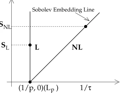
It is useful to have a pictorial description of smoothness spaces. We shall correspond smoothness spaces with points in the upper right quadrant of ¶·

¡

. Namely, a smoothness space consisting of functions of smoothness orderµ in 1¬ will be identified with the pointŸ.®7¸h˜°0µV¦ (see

Figure 3.1). This identification is coarse in the sense that several spaces are identified with the same point. For example all space ¨ 

¹

Ÿ+  ¬ Ÿ¥¤¦F¦ are identified with Ÿ.®7¸h˜1°0µV¦ irrespective ofº . We

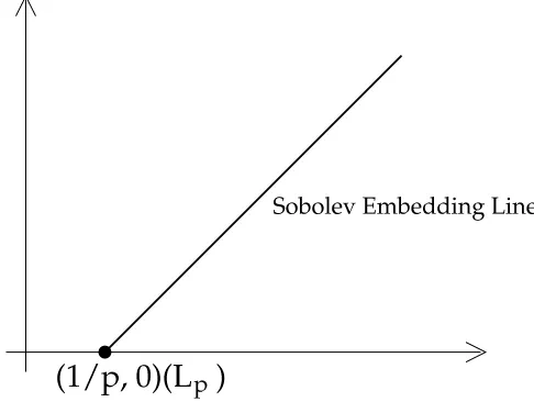
will come back to this picture often but at this stage let us just point out, as an example, how to interpret the Sobolev embedding theorem in this picture. The line with slope » passing through

Ÿ.®7¸h˜1°0¼¦ is the demarkation line for embeddings of Besov spaces into  ¬ Ÿ¥¤¦ (see Figure 3.1). Any

Besov space with primary indices corresponding to a point above that line is embedded into  ¬ Ÿ¥¤¦

(regardless of the secondary indexº ). Besov spaces corresponding to points on the demarkation

line may or may not be embedded in   ¬ Ÿ¥¤¦ . For example the Besov spaces ¨}½

Ÿ+ 

½

Ÿ¥¤¦F¦ with

®7¸b¾w™=µ¸b»À¿"®7¸h˜ correspond to points on the demarkation line and they are embedded in  ¬ Ÿ¥¤¦.

Points below the demarkation line are never embedded in 

¬

Ÿ¥¤¦.

Á Â Ã Â ÄÅ Æ Ç È Ã Å É É ÊË Ì Í ÊË Å

Î Ï Ð Ñ Ò Ó Ô Î Õ Ô

Ö

Ï Ð

τ

× Ø

Ø

Ù

Í

Ú

Í

Ù

Figure 3.1: Graphical interpretation of linear and nonlinear approximationŸ+»™>®7¦ .

4

Linear methods

After this short discourse concerning wavelets and smoothness spaces, let us return to our main thread of thought which is the understanding of when the solution to our PDE can be approximated

with a prescribed efficiency by linear or nonlinear methods. We begin with linear methods. Let us consider a functionè defined on a domainé>ê@ëìmí which is the solution to a PDE

which we wish to numerically resolve. We shall call è the target function. We shall consider

numerical methods which fix a sequenceîï of linear spaces whose dimension is of orderð and

approximateè by an elementñ ï-òèMó ofî ï . This type of numerical algorithm is said to be linear

because the approximantsñ ïò

è-ó come from the linear spaceî

ï which is fixed in advance (does

not change withè ).

To assess the performance of such a numerical algorithm, we would choose a norm ôõ2ô in

which we want to measure error. Typical choices are the energy norm or theö¢÷ norm for elliptic

problems, theöø norm for conservation laws, and theö³ù norm for Hamilton-Jacobi equations.

The error for approximatingè with this algorithm is measured by

ú

ïòè-ó³ûýüþô0è~ÿñ ïMòèMó7ô

(4.1)

As a benchmark for the performance of the numerical algorithm, it would be useful to compare this error with the ideal error

ï òèMó³ûýü

òèFîïó³ûýü

ô0è~ÿ ô

(4.2)

In some ideal cases, this is made with great success. For example, for elliptic problems in which

ñ ïMòèMó is the Galerkin approximation toè fromî ï , we have thatñ ïMòèMó is the best approximation

toè in the energy norm and so

ïò

èMó¢üþô0è|ÿñ

ïò è-ó7ô ü

ú

ïò è-ó

(4.3)

Let us consider our two main examples. Standard Finite Element Methods would begin with a sequence ò ï{ó of partitions ofé and a corresponding spaces-ïtûýü ò ï{ó of piecewise

polynomials on that partition. Typical assumptions are that é is a polyhedral domain and the

elements of the partition are simplices. To be useful, the space ï should admit a nice basis ò ó

with an accessible dual basis; usually coefficients in the representation ü ! , for a given

#"$ ï , are determined by nodal values of or its derivatives (their values at the vertices of the

partition). We assume that the dimension of

ï is of order ð .

In linear wavelet methods, we would fix a sequence% ï ê ,ð ü'&(*)+, of indexing sets

and consider the spaces ,

ï

ûýü.-0/21354687û:9;"<%

ï>=

We shall always assume that %ïxê'%ï(? ø , ð.@A& , so that the spaces

,

ï are likewise nested. A

typical choice is% ï to be the firstð wavelets in their natural order. The numerical method would

choose a value ofð then create an approximantB ïò

è-ó toè from

,

ï .

Given one of these linear methods of approximation and given our target function è , we

introduce the real numberCEDGFIH defined by the properties that for eachCKJICED ,

ï òèMóMLON@ðQPSR

(4.4)

and further for eachCTFICUD , V

WO-YX /

ï3Z ù

ð

R

ïMòèMó ü\[#

(4.5)

In otherwords, lUm is the supremum over all l satisfying (4.4). No numerical algorithm which

generates approximations fromnpo can provide approximationsq2o which provide accuracy better

thanrtsvuQwSxzy>{ .

How can we determine the value of l m for our target function q ? We call on our two

pillars: approximation theory and regularity theorems for PDEs. Let us first consider the role of approximation theory. For the statement of the following theorem, we fix a domain|}~€‚ on

which the PDE is posed and fix anƒ„>s|…{ norm†‡ˆ†‰„ withŠ‚‹Œ<‹# in which we shall measure

error. Similar results hold when the error is measured in a Sobolev or Besov norm.

The following generic theorem holds for a variety of settings which we shall dilineate in a moment:

Theorem 4.1 There is a real numberŽO‘ , such that for any‘’#lT’“Ž , we have that a function ”–•

ƒ—„ s|…{ satisfies ˜

s

”2™

npo2{v„‹Oš›u wSxzœ



™

užŸŠ

™* ¡™¢¢¢E™

(4.6)

if and only if”

is in the Besov space£px

¤

sƒ—„>s|…{0{ .

When it applies, this theorem completely characterizes the functions which can be approximated with orderr¥svu

wSx

{ . It says that to achieve this error it is necessary and sufficient that

”

hasl orders

of smoothness inƒ—„ .

Theorem 4.1 holds in a variety of settings. We discuss the two main settings of interest to us in this talk. If¦§o denotes the wavelet space spanned by the firstu wavelets in the wavelet basis

forƒ©¨3s|…{ (seeª 2), then this theorem holds withŽ!\«¥¬­bsv®

™0¯

{ with® the number of vanishing

moments of the wavelets and¯

the smoothness of the wavelets as measured inƒ„>s|…{ ( the wavelet

should be in£°

¤

sƒ„>s|…{).

The situation for approximation using piecewise polynomials is a little less clean. In fact, spaces±²s³o { of piecewise polynomials of fixed degree which are defined by continuity

assump-tions across the boundaries of the simplicies´ are not completely understood from the standpoint

of their dimension or approximation properties. On the other hand, the spaces used in FEM all have stable bases which form good partitions of unity and the following remarks apply to approx-imation from these spaces (see [2])

We assume that³o is a partition of a fixed polyhedral domain into a collection ofu

sim-plicies ´ . We assume that this simplicial decomposition is more or less uniform and that each

simplex ´

•

³o satisfies the shape condition. This means that there are balls £

°

and £¶µ of

radius¯

and€ respectively such that

£

°

}“´\}O£¶µ

(4.7)

and ·¹¸

‹

€

¯

‹

·Uº*·¹¸

u

w

º

œ

 ‹“Ž‹O€Ÿ‹

·Uº

u

w

º

œ



(4.8)

with absolute constants

·¹¸

™

·Uº

»‘ . Let±boG¼½\±²s³po:{ be a linear space of piecewise polynomials

of fixed degree® subordinate to ³o which admits a good partition of unity in the sense of [2].

Then, Theorem 4.1 holds for n o ¾± o andŽ¼½¿«¥¬À­Ásv® Š ™0¯

{ where

¯

is the smoothness of the elements Ã

•

±bo as measured in ƒ—„ (each à is assumed to be in £ °

¤

sƒ—„>s|…{). The generic

theorem holds for a larger range of Ð if the partitionsÑÒ are not nested but rather satisfy certain

mixing conditions (see [10] for a discussion of this).

One should not underestimate the power of Theorem 4.1. It is an if and only if theorem. Not only does it give a sufficient condition (ÓÕÔ#֐×

Ø;ÙڗÛ>Ù܅Ý) for approximation of

Ó to be bounded

byޛßQà × , it also says that ifÓ does not satisfy this smoothness condition then there is no hope in

achieving this approximation order.

How do we utilize this theorem in our search for the numberÐEá for our solutionâ to the

PDE. What we need to determine is the maximum value of Ð for whichâ lies in the Besov space

֐×Ø ÙڗÛ>Ù܅Ý0Ý . This has a simple interpretation in our picture of smoothness spaces. We fix the point

ÙkãUä*åæYçˆÝ (which corresponds toÚ Û ) and consider the verticle line passing through this point which

therefore consists of all points of the form ÙkãUä*å—æ

Ð

Ý. We search along this line for the maximum

value ofÐ , such thatâ is in the corresponding Besov space. This determinesÐEá (see Figure 4.2).

Î Ï Ð Ñ Ò Ó Ô Î Õ Ô

Ö

Á Â Ã Â ÄÅ Æ Ç È Ã Å É É ÊË Ì Í ÊË Å

Figure 4.2: Graphical interpretation of linear and nonlinear approximation.

It is the role of regularity theorems for PDEs to provide us with the answer to this question. We shall return to this topic later in this talk after we have introduced the concepts needed to determineÐEèéá for nonlinear approximation.

5

Nonlinear methods

Let us now consider nonlinear numerical methods for recovering the solution â . In this case,

the numerical method no longer generates an approximation from a linear space (prescribed in advance) but rather a nonlinear manifold ê+Ò where the dimension (number of parameters) of ê+Ò

is of orderß . Similar to the linear case described above we can define the ideal error

ë

Ò

Ù

Ó

Ý+ì½í îï>ð

ñò(ó ôöõ Ó!÷$ø

õ

(5.1)

where

õ©ù:õ

is the norm we have chosen to measure error.

Given our target function , we define to be the the real number such that

! #" $&%'"

(5.2)

for all)(* and +-,-./021

4365 7

98:%

(5.3)

for all)* . Approximation theory will tell us the conditions on which determine .

Let us begin with the wavelet case in which the results are very precise. An adaptive wavelet method generates an approximation to from the set;

which consists of all functions< of the

form

<=8?>

@4ACBED @GFH@

(5.4)

where the cardinality IKJ ofJ is L . This is called n-term approximation and recent results

[11] (see also [5]) characterize its approximation properties. To describe these, we introduce the sequence D#M ON P 5 4QSR

which is the nondecreasing rearrangement of T

D @ ON T @4ACU

. In other words,

D M

ON

is the -th largest of the

T D @ ON T

, VXWZY . The following theorem characterizes the functions

which can be approximated to rate[

!

by -term wavelet approximation.

Theorem 5.1 LetK(]\('% . A function

N W_^7` ba ( N Wc6` ba

if\_:d ) satisfies

ON O`ef ON g ! (5.5)

if and only if the rearranged wavelet coefficients ofN

satisfy D M ON Eh ON g ! Rgi ` " _8?d4"jk"#l#l#lC" (5.6)

for some constant

h

ON

. Moreover, the smallest constant ON

in (5.5) is equivalent to the

smallest constant h ON

satisfying (5.6).

Let us denote bym the space of functions

N

satisfying (5.6). This is not a classical smooth-ness space (Besov or Sobolev space) but it is very close to requiring thatN

has orders of

smooth-ness in^onp gq withr 4st8 4uCvxwydzu\{ R

. In fact, we have the embeddings

| np gq ^ nCp }q ba PE~fm ~ | P€ nCp €q ^ nCp €bq ba P‚" (5.7)

where ƒ„… is arbitrary. There are also more precise connections between approximation rates

and Besov spaces (see [10]).

Theorem 5.1 is enough for us to describe how to determineC for our target function .

We look at the scale of Besov spaces | nCp gq ^9nCp }q ba

P , r

C„8 CuCv„w†dzu\{ R

, =‡ . These

spaces are nested and strictly decrease as increases. ThenCo is the supremum of all the for

which is in| nCp }q ^ nCp }q ba P.

This all has a nice interpretation in our picture of smoothness spaces (see Figure 4.2). We fix the ^7` norm in which we shall measure the error. This identifies the point

dzu\7"ˆ . The

spaces| nCp }q ^onCp }q ba

P all live on the line emanating from

dzu\7"ˆ with slopev . Thus, starting at

—˜z™š7›œˆ

we move on this line as long asž is in the corresponding Besov space and stop whenž is

not in this space. This identifies the numberŸC ¡ .

We shall not give a precise formulation of the corresponding results for adaptive Finite Ele-ment Methods except to say that the story is roughly the same as in the wavelet case. Such adaptive methods begin with a polyhedral domain¢ and an initial decomposition£E¤ of¢ into simplicial

cells ¥ . The adaptive procedure begins with the initial triangulation £ ¤ and iteratively refines

simplicies. Thus, at the first iteration we generate a partition £§¦ which is obtained from £¤ by

refining some of the simplices in£ ¤ and not others. In general£H¨‚© ¦ is gotten from£H¨ in the same

way. If the adaptive strategy (i.e. the selection of simplicies which are to be subdivided) is chosen correctly and if the resulting space of piecewise polynomials allows for good local bases then it is possible to prove that whenever ž is in the Besov spaceªK«¬C­

«g® —¯

¬C­

«}®



, it will be approximated

with the efficiency ° —O±²

«}³´



with

±

the number of simplices in the resulting partition. Inverse estimates can be proven if the refinement strategy guarantees the shape preserving property of the simplicies in£H¨ for eachµ . For precise formulations of the above and for details we refer to the

forthcoming paper [1].

6

The theory in action

We have seen that to determine whether it is beneficial to use nonlinear methods to approximate our target functionž we need to determine the two numbersŸ ¡ andŸ  ¡ associated tož and check

whether Ÿ ¡·¶¸Ÿz¡ . We do this by checking the regularity ofž in the two scales of smoothness

spaces associated to linear and nonlinear approximation. A result which determines the regularity of ž in one of these scales is called a regularity theorems for PDE’s. A typical regularity

theo-rem infers the smoothness of the solution ž to a PDE from information in the PDE such as the

coefficients, inhomogeneous term, initial conditions, or boundary conditions.

To illustrate how this theory plays out in specific settings, we shall consider two model problems; one hyperbolic and the other elliptic.

6.1 Conservation laws

Consider the scalar univariate conservation law

¹

ž€º!»·¼

—

ž

g½6¾¿œ ÀÁ_ÂÃK›ÅÄ

¶

œÆ›

ž

—OÀ7›œˆ¾

ž!¤

—OÀ{ ÀÁ_ÂÃK›

(6.1)

where¼ is a given flux,ž

¤ a given initial condition which will assume is of compact support, and ž is the sought after solution. This is a well-studied nonlinear transport equation with transport

velocityÇ

—

ž

o¾

¼ÉÈ

—

ž



. We shall assume that the flux is strictly convex which means the transport velocity is strictly increasing. The important fact for us is that, even when the initial conditionž ¤

is smooth, the solutionž —}ʍ›Pĝ

will develop spontaneous shock discontinuities at later times

Ä

. The proper setting for the analysis of conservation laws is in

¯

¦ and in particular the error of

numerical methods should be measured in this space. Thus, concerning the performance of linear numerical methods, the question arises as to the possible values of the smoothness parameter Ÿ¡

of×Ø}ٍÚPÛPÜ as measured inÝßÞ . It is known that if the initial condition×!à is ináâ , then the solution

× remains in this space for all later time Û6ãåä (note thatáâçæåè

Þ

é

؁ÝßÞ؁êë)ÜPÜ ). However, since,

for any initial condition, this solution develops discontinuities, the Sobolev embedding theorem precludes × being in any Besov space èKì

é

ØÝ Þ ÜPÜ for any íîãðï . This means that the largest

value we can expect for íñ is íñ?òóï and we get this value whenever ×Éà·ô…áâ . Thus, the

optimal performance, we can expect from linear methods of approximation is õ„ØOö÷

Þ

Ü with ö

the dimension of the linear spaces used in the approximation. Typical numerical methods utilize spaces of piecewise polynomials on a uniform mesh with mesh length ø and the above remarks

mean that the maximum efficiency we can expect for such numerical methods is õ„ØbøÉÜ, ø…ù

ä . In reality, the best proven estimates are õ„Øgú øÉÜ under the assumption that×!àûôåáâ . This

discrepancy between the possible performance of numerical algorithms and the actual performance is not unusual. The solution is known to have sufficient regularity to be approximated, for example, by piecewise constants with uniform meshø to accuracyõ„Øbø!Ü but algorithms which capture this

accuracy are generailly not kown.

To understand the possible performance of nonlinear methods such as moving grid methods, we should estimate the smoothness of the solution in the nonlinear Besov scale èeìüCý

ì}þ ؁Ý

üCý

ìgþ Ü ,

ÿ

ØbíCÜtò Øbí

ïzÜ÷

Þ

, corresponding to approximation in the ÝßÞ-norm. A rather surprising result

of DeVore and Lucier [12] shows that starting with any initial condition× à of bounded variation

which is in this space, the solution × will remain in this Besov space for all later timeÛ ã ä .

In particular, if ×!à is

é

with compact support then this means that nonlinear methods such as moving grid methods could provide arbitrarily high efficiency. In fact, such algorithms, based on piecewise polynomial approximation, can be constructed using the method of characteristics (see Lucier [14] for the case of piecewise linear approximation).

In summary, whenever the initial condition×!à is of bounded variation and in the smoothness

spaceèeìüý ìgþ

ØÝ üCý

ì}þ

ÜPÜ withí ã?ï , then the use of adaptive methods is justified sinceí ñ ã¿í ñ . In

particular, if×Éà is of bounded variation and in

é

thení ñ ò whileíñ ò?ï .

6.2 Elliptic equations

An extensive accounting of the role of linear and nonlinear approximation in the solution of elliptic problems is given in Dahmen [8] and Dahlke, Dahmen, and DeVore [6]. We shall therefore limit ourselves to reiterating a couple of important points about the role of regularity theores and the form of nonlinear estimates. We consider the model problem

× ò on yæ*êëGÚ

(6.2)

× ò ä on

of Laplaces equation on a domain æ êë with zero boundary conditions. This equation is

closely related to the Dirichlet problem for harmonic functions on :

ò ä on yæêë

Ú

(6.3)

ò on

We shall also limit our discussion to estimating error in theÝ -norm. These results extend trivially

to approximation in the Sobolev space ·ò{ØÝ Ø ÜPÜ and in particular to the caseåò ï

which is equivalent to the energy norm for (6.2). There are also various results known for general

0

[13].

Consider first the case where132465879;: and9 has a smooth boundary. Then, the solution

<

to (6.2) has smoothness =

5

7>4 5 79;:-: and can therefore be approximated by linear spaces of

piecewise polynomials of dimension? to accuracy @A7B?DC 5FEHG

: . This accuracy can be obtained by

using standard FEM with uniformly refined partitions.

If the boundary IJ9 of9 is not smooth then the solution

<

to (6.2) has singularities due to corners or other nonsmoothness of the boundary IJ9 . For example for Laplace’s equation

on a general Lipschitz domain, we can only expect that the solution <

is in the Sobolev space

=LK EH5

7>465879;:-: . Thus, in general, we can at most expectMONQPSRUTWV .

Because of the appearance of singularities due to the boundary, adaptive numerical tech-niques are suggested for numerically recovering the solution<

. We understand that to justify the use of such methods, we should determine the regularity of the solution in the scale of Besov spacesXZY[\

Y^] 7>4

[\

Y_]

79;:-: , `a7M:ZbcPd7MfegOTWVU:hC%i . Such regularity has been studied by Dahlke and

DeVore [7]. They prove, among other things, that for any Lipschitz domain the nonlinear smooth-ness Mkj

N associated to

<

always exceeds the linear smoothness. Namely, Mj

Nml K

G

5

\

G

C%i^]

M

N . In

other words, the use of nonlinear adaptive methods for numerically recovering the solution<

to (6.2) is theoretically justified.

7

An adaptive algorithm for elliptic problems

Up to this point, we have not discussed the properties of any specific numerical algorithm but rather have addressed the question of whether nonlinear or adaptive algorithms could possibly be of benefit in numerically approximating the solution of a PDE. Even if we have decided that an adaptive method should be of use, there remains the problem of constructing an adaptive algorithm which exhibits the expected performance. This is indeed a nontrivial task. We shall close this talk by discussing the recent wavelet based adaptive algorithm given in [4] which has been proven to exhibit optimal performance in the sense of providing the best allowable rate of approximation to

<

.

7.1 The setting

Let9 be a domain (or manifold) inno

G

and letp be a linear operator mappingq intoqr where

q is a subspace with the property that eitherq or its dualq r is embedded in45U79f: . The operator p induces the bilinear forms defined onqutvq by

sw7 <yx-z

:{bcP}|>p <yx-z~(x

(7.1)

where|_€

x

€

~

denotes the7>qr

x

q: duality product. We assume that the bilinear forms is symmetric

positive definite and elliptic in the sense that

s7 zJx-z

:6‚„ƒ

z

ƒ

5 …

x†z

2‡q‰ˆ

(7.2)

It follows that — is a pre-Hilbert space with respect to the inner product ˜ and that this inner

product induces a norm (called the energy norm) on— by

™š™h›œžcŸ

˜w  š#¡¢šc£(¤

(7.3)

The energy norm is equivalent to

™6š™(¥

. By duality,¦ thus defines an isomorphism from— onto

—§ .

We are interested in numerically recovering the solution¨ to the elliptic equation

¦f¨ Ÿ©

(7.4)

with

©ª

— § . It follows that¨ is also the unique solution of the variational equation

˜w B¨

¡-«¬£Ÿ}­©¡-«¬®(¡°¯B±8²´³8µŽµZ«ª

—

¤

(7.5)

The typical examples included in the above assumptions are the Poisson or the biharmonic equations on bounded domains in ¶·¸ ; single or double layer potentials and hypersingular

opera-tors on closed surfaces arising in the context of boundary integral equations. In these examples—

is a Sobolev space, e.g. —

Ÿ —°¹ º  » £ ,— › º  » £

, or—

Ÿ —½¼%¹^¾ ›  » £ (see [8]).

The numerical methods developed in [4] require the existence of a biorthogonal wavelet basis ¿ for» . The wavelets in ¿ are in— , whereas those in the dual basis ¿À are in— § . Thus,

each

ǻ

— has a wavelet expansion «ZŸSÁaÂ

¿ (with coordinatesÃÅÄ Ÿ}­B«¡

À

Æ

Ä

®

). We assume that

™hÇ ¼%¹ ÁșHÉ^Ê(ËÍÌÏÎÑЄ™hÁ  ¿ ™(¥Ò¤ (7.6) with Ç

a fixed positive diagonal matrix. Observe that (7.6) implies that

Ç ÄWÓÄ Ð„™ Æ Ä ™ ¼%¹ ¥

, and that

¿ (resp. Ôv¼%¹(¿ ) is an unconditional (resp. Riesz) basis for— . By duality, one easily obtains that

each

ǻ

— § has a wavelet expansion

«ÕŸSÁ Â

À

¿ (with coordinatesÃÅÄ Ÿ}­B«¡

Æ

Ä

®

) that satisfies

™hÇÖÁ;™ É^Ê!ËÍÌÏΠЄ™hÁ  À ¿ ™ ¥Ø× ¤ (7.7)

We also assume that the wavelet bases ¿ and ¿À provide characterizations of Besov and

Sobolev spaces (as described earlier) for a suitable range of the smoothness parameter. In the context of elliptic equations, — is typically some Sobolev space—‰Ù

Ÿ„Ú

ÙF >Û

›

 » £-£

. In this case the above assumptions are satisfied whenever the wavelets are sufficiently smooth, with

Ç ÄWÓÄ Ÿ Ü ¼yÝ Ä

ÝÙ. For instance, when¦ ŸßÞfà

, one hasá Ÿ}â

.

If we write the unknown solution¨ and the right hand side

©

in terms of their wavelet bases we obtain an infinite system of equations. After preconditioning using the matrix ã , we obtain

from (7.5) the system of equations:

Ç°­

¦¿

¡

¿

® Â ÇÖÇ

¼%¹

ÁŸäÇ°­©¡

¿

® Â ¡

(7.8)

or more compactly, åQæ ŸäçU¡ (7.9) where å cŸÇ°­ ¦¿ ¡ ¿ ®  Ç3¡ æ cŸäÇ ¼%¹ Á¡‰çècŸäÇ°­©¡ ¿ ®  ªvé ›  ê £(¤ (7.10)

The matrixö is symmetric positive definite.

One can show that in all classical settings for elliptic problems, the matrixö satisfies certain

sparsity conditions. These arise from the fact that

÷Åø%ù>úû¢üBúýDúûþúÿ

û ü û

÷Åøyúúûþúøyúû¢üúú

!hø#" (7.11) with$&% ('W÷ and)&% and *

+-,S÷/.1032 ùBúûþú4úû üúÿ65#798!: 8<;=#= >

û 8<;#=#= > û ü !@? (7.12)

We refer the reader to [8] for a discussion of the various settings in which (7.11) is known to be valid.

7.2 The numerical method

To numerically resolve (7.4), we use the Galerkin method. We fix a finite setA of wavelet indices

and approximateB from the spaceC*D

+-, 8!=E6F >

û

+HG

A I . The approximate Galerkin solution B D fromC D is defined by the conditions

J

B D !K L,MON !K PRQ ùTSÿ K G C D ? (7.13)

In matrix form, this is equivalent to solving the finite matrix problem

öUDWVXD ,ZY

D

(7.14)

whereöUD is the finite section ofö gotten by choosing the rows and columns ofö corresponding

toA , VXD is the unknown vector (which determines the wavelet coefficients ofBD ), and

Y

D is the

vector obtained by restrictingY

toA .

The numerical method studied in [4] proceeds as follows. It starts with an initial setA[ of

wavelet indices (one may takeA [ ,]\

) and given that a setA_^ has been chosen, it generates a new

setA

^

ýa` with hoefully better approximation properties.

Let us describe the two main steps for determining the setA

, A ^ ýa` from A +-,

A ^ which

work from the discrete equations (7.9). Let VXD be the current vector solution to (7.14). We can

view VXD as a vector defined for all bGZc

by defining V

û

,ed

, bGZcgf

A . Then the residual

h D +-, ö VjikV D l,ZY

i´ömV D has norm

n h D no Q ùpDÿ (7.15)

that can, by the ellipticity assumptions, be related to the function error

n

BmiqBD n@r

. Note thath

D

vanishes onA . The set A

is obtained as follows. First, we enlargeA to a setAs containingA by

adjoining the wavelet indicies whereh

D is large. We adjoin a finite set of verticesAs

f

A so that this

set captures at least half of the energy ofh

D . We next solve the Galerkin problem on the new set

s

A resulting in the new vectorVut

D . We examine the entries in Vut

D and put into

A

only those indices whose keep are sufficiently large. This step can be viewed as thesholding the entries inVvD .

In practice, the algorithm is implemented by choosing anwx%

d

and an initial setA[ and

generating sets A_^ ,y ,z

÷

{ ?{?{?

, until the error tolerance w is guaranteed. Note that the error at

any given stage is upper bounded by a fixed multiple of the norm of the residual.

7.3 Performance of the algorithm

The results in [4] show that the above algorithm has optimal performance in the following sense. Suppose that the solution Š to (7.4) can be approximated (in the energy norm) with ‹ wavelets

terms to accuracy Œ#Ž

Š‚‘“’”‹_•–{— ‹™˜Mš›—œ(—{{{ž—

(7.16)

with’ an absolute constant. Then, for eachŸ¡ ¢š , the above numerical algorithm will generate

an approximationŠ£¥¤ with

¦

Š¨§&Š £¥¤ ¦©

«ª¬’®­¯•–

°

(7.17)

with­ °²±

˜®³²´

°

the cardinality of´

°

. Moreover, the number of arithmetic operations necessary to find´

°

and to computeŠ £¥¤ will not exceedª¬­

°

. The number of sorting operations necessary in the thresholding portion of the above algorithm does not exceedªµ­

°‚¶€·6¸

­

°

.

The proof of this result is nontrivial and we shall only mention a few of the key ingredients in the proof in the following remarks.

Remark 1. Capturing at least half of the energy in the residual¹ £ guarantees that the new

Galerkin solution on´º reduces the error by a fixed factor»m¼½š :

¦

Š¨§&Š‘¾

£

¦@¿

À»

¦

Š¨§&Š £ ¦@¿



(7.18)

This result would lead, in and of itself (without thresholding), to a convergent algorithm but would not sufficiently control the number of entries in the sets´º

°

.

Remark 2. In numerical implementation of the algorithm, it is necessary to limit the search

for the entries which need to be adjoined to ´ in order to obtain´º . Here the sparseness of the

matrixÁ plays a crucial role.

Remark 3. The thresholding step when employed with the correct threshold reduces the

number of elements used in the approximation without seriously effecting the error. This is proved by establishing a general result on thresholding.

Remark 4. To bound the number of arithmetic operations requires fast methods for

multi-plying a sparse matrix ( in our caseÂØ¢Á ) with a sparse vectorÄ (in our caseÄŘMÆ £ ) (see

[4] for the interesting method to do this).

References

[1] P. Binev, R. DeVore, and P. Petrushev, Adaptive approximation using piecewise polynomials, in prepa-ration

[2] C. de Boor and R. DeVore, Partitions of unity and approximation PAMS, 93 (1985), 705-708.

[3] A. Cohen, Wavelet methods in Numerical Analysis, to appear in the Handbook of Numerical Analysis, vol. VII, 1998.

[4] A. Cohen, W. Dahmen, and R. DeVore, Adaptive wavelet methods for elliptic operator equations: convergence rates, to appear in Math. Comp.

[5] A. Cohen, R. DeVore, and R. Hochmuth Restricted approximation, Constructive Approximation, 16 (2000), 85–113.

[6] S. Dahlke, W. Dahmen, and R. DeVore, Nonlinear approximation and adaptive techniques for solving elliptic equations, in: Multiscale Techniques for PDEs, W. Dahmen, A. Kurdila, and P. Oswald (eds), Academic Press, 1997, San Diego, 237–284.

[7] S. Dahlke and R. DeVore, Besov regularity for elliptic boundary value problems, Communications in PDEs, 22(1997), 1–16.

[8] W. Dahmen, Wavelet and multiscale methods for operator equations, Acta Numerica, 6(1997, Cam-bridge University Press, , 55–228.

[9] I. Daubechies, Ten Lectures on Wavelets, CBMS-NSF Regional Conference Series in Applied Mathe-matics, 61, SIAM Philadelphia, 1988.

[10] R. DeVore, Nonlinear approximation, Acta Numerica 7 (1998), 51-150.

[11] R. DeVore, B. Jawerth and V. Popov, Compression of wavelet decompositions, Amer. J. Math., 114 (1992), 737–785.

[12] R. DeVore and B. Lucier, High order regularity for conservation laws, Indiana Journal of Math., 39 (1990), 413–430 .

[13] Jerison and Kenig, The inhomogeneous Dirichlet problem in Lipschitz domains, J. of Functional Anal-ysis, 130(1995), 161–219.

[14] B. Lucier, Regularity through approximation for scalar conservation laws, SIAM J. Math. Analysis, 19(1998), 763–773.

[15] Y. Meyer, Ondelettes et Operateurs, Vol 1 and 2, Hermann, Paris, 1990

Ronald A. DeVore

Department of Mathematics University of South Carolina Columbia, SC 29208 USA

e–mail:[email protected]

http://www.math.sc.edu/Ô devore/