Please cite this article as: M. Forghani, M. A. Vahdat-Zad, A. Sadegheih, Developing the Inventory Routing Problem with Backhauls, Heterogeneous Fleet and Split Service, International Journal of Engineering (IJE), IJE TRANSACTIONS C: Aspects Vol. 31, No. 6, (June 2018) 949-958
International Journal of Engineering
J o u r n a l H o m e p a g e : w w w . i j e . i rDeveloping the Inventory Routing Problem with Backhauls, Heterogeneous Fleet and
Split Service
M. Forghani, M. A. Vahdat-Zad*, A. Sadegheih
Department of Industrial Engineering, Faculty of Engineering, Yazd University, Yazd, Iran
P A P E R I N F O
Paper history: Received 30 July 2017
Received in revised form 08 January 2018 Accepted 15 February 2018
Keywords: Inventory-routing Backhauls Logistics
Heterogeneous Fleet Split Delivery Genetic Algorithm Multi Product
A B S T R A C T
One of the most important points in a supply chain is customer-driven modeling, which reduces the bullwhip effect in the supply chain, as well as the costs of investment on the inventory and efficient transshipment of the products. Their homogeneity is reflected in the Inventory Routing Problem, which is a combination of distribution and inventory management. This paper expands the classical Inventory Routing Problem based on the Multiple Delivery Strategy along with one of the functionalities of routing problem, namely, "backhauls", with a priority consideration for linehaul customers. Then it has been modeled in the form of a problem with Multi-period, multi-product, and multi- vehicle planning horizons in which stock out is not allowed. Moreover, for an optimal use of the vehicle capacity to serve the linehaul and backhaul customers, this study adopted a “split service” problem to the model, which also increases the complexity of the problem. First, considering the above-mentioned assumptions, a new mathematical model is proposed in the form of mixed integer programming for the problem defined in this paper. Then, since the stated problem can be considered among the non-deterministic polynomial-time hard, an efficient meta-heuristic genetic algorithm is provided for solving it. At the end, the numerical results obtained by this algorithm are analyzed using the randomized test problems. The result shows that by adopting a split service approach, 70% of the test problems will demonstrate cost reduction.
doi: 10.5829/ije.2018.31.06c.12
1. INTRODUCTION1
In the recent years, a great consideration has been made on coordination, Co-operation, and integration of the various elements of the supply chain in order to achieve a competitive advantage. Transportation is one of the key elements in supply chain. And a proper design of a transportation network results a better performance of the system. One of the other goal of SCM is to keep the inventory throughout the chain minimized. Therefore, the distribution issue also has a great importance. The coordination between the inventory and routing in the distribution systems can be considered as a kind of coordination among the components of the supply chain.
The Inventory Routing Problem (IRP) is raised when inventory and vehicle routing need to be considered
*Corresponding Author’s Email: [email protected](M. A. Vahdat-Zad)
simultaneously [1]. The precise and ultimate goal of the Inventory Routing Problem is to determine the distribution strategy in order to reduce the long-term distribution costs, and make the supplier decide on when the customer is to be visited, how much product should be delivered to the customer, and how to route and plan the customers in the form of a tour. The IRP with backhauls can be considered as the improved form of the classical Inventory Routing Problem that can be efficiently applied in the real world problems.
heterogeneous fleets with limited but varying capacity, using the split service strategy. On the other hand, considering the backhauls, the customers are divided into two categories of line haul customers and backhaul customers, the line hauls being always the preferred ones. Meanwhile, the vehicles always move from the central depot (distributor), and after visiting one or more customers return to the same station. Since the Inventory Routing Problem involves the VRP as a sub-problem, and since the VRP is NP-hard [2], it can be concluded that the IRP problem is also strongly NP-hard. Therefore, it is needed to use the meta-heuristic algorithms to find the appropriate solutions at a reasonable computational time. In this paper, also an effective genetic algorithm is proposed to solve the model. The efficiency of the algorithm is tested with the results attained by GAMS software.
Considering the above-mentioned ideas, the present study has explored the theoretical foundations and literature of the discussed issue in section 2, and section 3 of the paper is devoted to the provision of the mathematical modeling of the defined problem. In section 4, the proposed meta-heuristic algorithm for solving the problem is described. In order to analyze the results, the computational results obtained by the implementation of the proposed algorithm for the defined problem are provided in section 5. Finally, in section 6, the conclusion and the recommendations for future research are presented.
2. LITERATURE REVIEW
The first published studies on IRP have been devoted to changing the model designed for VRP and the heuristic developed considering the inventory costs. The base study of Bell et al. just covers the transportationcosts, in which the demand is stochastic and a specific level of the customer’s demand needs to be provided [3].
Given the importance of each of the different parameters for the researchers, they have presented different categories for IRP problems. For example, Kleywegtet al. considered four key elements that include: 1- Demand, 2-Fleet size, 3- Time horizons, and 4-Types of the delivery. They examined the random Inventory Routing Problem with direct deliveries and the problem is presented in the form of Markov decision-making process in a discrete-time period [4]. Andersson et al. [5] divided the IRP problem based on seven factors: 1- Time horizon, 2-Demand, 3- Topology, 4- Type of routing, 5. Inventory management decisions, 6 –Fleet composition, and 7- Fleet size [5]. Eventually, taking into account all the studies that had been done up to that time, Coelho et al. [6] provided a standardized classification for IRP problems. This classification, initially, provided a seven-factor cluster
for the basic IRP problems, including: 1- Time horizons 2-Structure3-Type of routing 4- Inventory policy 5- Inventory decisions (back orders, lost sales, and non-negative inventory) 6- Fleet composition, and 7- Fleet size. Then the problems developed out of the classical IRP problems were introduced (including production-routing-inventory, multi-product problems, location-routing-inventory, etc.). Finally, the Inventory Routing Problem were classified in terms of the type of the demand (deterministic or stochastic) [6]. In this study, the literature on of some of these features that are used in the definition of the problem, such as multi-production, multi-vehicle, proposed solving method, split service, etc., will be discussed.
In the case of Inventory Routing Problems with multi-vehicles (MIRP), Coelho et al. [7] and Adulyasak et al. [8] used the exact method of branch and cutto solve their problem. Coelho et al. used the meta-heuristic algorithms of adaptive large-scale neighborhood search combined with theexact method of mixed integerlinear programming, for multi-vehicleInventory Routing Problems [9]. Santos et al. presented a hybrid heuristic algorithm based on aniterated local search for multi-vehicleInventory Routing Problem [10].
Considering the application of the meta-heuristic methods for multi-vehicle Inventory Routing Problems, one can use the efficient hybrid genetic algorithm reported in literture [11] and a two-step search, developed by Mjirda et al. [12], for period multi-productInventory Routing Problems. This two-step search consists of Variable Neighborhood Descent and Variable Neighborhood Search algorithm. In these studies, a many to one topology is used and each supplier provides one kind of product. A work similar to this kind of replenishment can be observed in literture [13]. Popović et al. [14] defined a period, multi-product problem in the field of fuel deliverycontaining homogeneous vehicle fleet and deterministic demand. Then, they proposed the meta-heuristic method of Variable Neighborhood Search to solve this problem.
The multi-vehicle multi-product Inventory Routing Problem was first proposed by Coelho and Laporte [15]. They proposed a mixed integerlinear programming for it, and used the exact branch and cut method to solve it.
problem, they divided the decision making process intotwo sub-processes:a- the planning and b-routing, and trying to integrate them using the mixed integer linear programming. The point worth noting, is that, in this model, each customer has a special storage location for each product and all the products cannot be stored in one place. Thus, each vehicle still carries only one type of product and the supplier will not have a limited capacity to store the products [16]. An algorithm based on a reduce and optimize approach (ROA) is developed for multi-product multi-period inventory lot sizing with supplier selection problem by Cárdenas-Barrón et al. [17].
There are some studies regarding the application of meta-heuristic methods for Inventory Routing Problem, such as the combination of genetic and particle swarm optimization [18], simulated annealing and tabu search [19], genetic algorithm with the design of Taguchi experiments [20], A hybrid heuristic model combining dynamic programming, ant colony optimization and tabu search has been proposed to solve a collaborative model for reverse supply chains and the optimization problem is modeled in terms of an inventory routing problem reported in literature [21], and also the particle swarm algorithm by Liu et al. [22]. Fattahi et al. proposed NSGAII and NRGA approach for bi-objective Production inventory routing problem with perishable product [23].
Concerningthe Inventory Routing Problems with split service, Yu et al. proposed a single-product IRP
problemwith the stochastic demand andthe
homogeneous vehicles fleets in the form of thesplit service. Using the Lagrangeanrelaxation, they divided the problem into two sub- problems and used linear programming and minimum costflew method to solve them, respectively [24]. Besides, Yu et al. [25] provided a model for Inventory Routing Problem with a fixed-deterministic demand and single product in which the transportations were split. The transportations fleet is homogeneous and limited in its capacity. Yu et al. [26] expanded their proposed model defined earlier into a stochastic demand one. This paper is different from their previous studies, due to the nonlinearity of the objective function, the consideration of the constraints such as the level of service provisionvwhich is also nonlinear, as well as the solving approaches.
3. PROBLEM DESCRIPTION AND MATHEMATICAL MODEL
According to the explanations provided in section 2 and the defined assumptions, the mathematical model of the MMIRPBSD problem, in which the stock out is not allowed, the capacity of the supplier is considered unlimited and the capacity of the customer's warehouse
is limited, is represented in the form of a mixed integer programming as follows:
3. 1. Indices
𝑁 : The set of total Customers N = {1,2, … , r, r + 1, r + 2, … , r + b}
𝑖 , j, 𝑢, e :Indices for customers (retailers) or Distributer (Supplier) that 0 and r + b + 1 denote the distribution center nodes.
𝑣: Index for vehicles 𝑉 = {1,2, … , 𝑣}
𝑝: Index for products P = {1,2, … , p}
𝑡: Index for Planning Periods T = {1,2, … , t}
𝑟: Index for linehaul customers R = {1,2, … , r}
𝑏: Index for backhauls customers B = {r + 1, … , r + b}
3. 2. Input Parameters
𝑓𝑣𝑡: A fixed cost for vehicle of type 𝑣;in periodt (𝑣 ∈ 𝑉)
𝑔𝑣𝑡: A cost per distance unit for vehicle of type 𝑣; (𝑣 ∈ 𝑉)
𝑞𝑖𝑣𝑡: The demand of the linehaul customer i∈R for product p ∈P in period t ∈ T
𝑅𝑖𝑣𝑡: The demand of the backhaul customer i∈B for product p ∈P in period t ∈ T,
𝑄𝑣: Weighted capacity of vehicle of type 𝑣; (𝑣 ∈ 𝑉),
𝑑𝑖𝑗: Distance between costumer 𝑖 and 𝑗for ∀(𝑖, 𝑗) ∈ 𝑁;𝐶𝑆𝑖𝑝: Holding cost per unit of product p ∈P at node i∈
N
𝑤𝑝: Weight of product p ∈P,
𝐶𝐶𝑖: Weighted storage capacity of customer i,
𝑀: A very big number,
3. 4. Model Formulation
𝑀𝑖𝑛(∑ ∑ ∑𝑃 𝐶𝑆𝑖𝑝. 𝐼𝑖𝑡𝑝 𝑝=1 𝑟+𝑏 𝑖=1 𝑇
𝑡=1 +
∑𝑡=1𝑇 ∑𝑟+𝑏𝑖=0∑𝑟+𝑏+1𝑗=1 ∑𝑉𝑣=1𝑑𝑖𝑗. 𝑔𝑣𝑡. 𝑧𝑖𝑗𝑣𝑡 (1)
+ ∑ ∑ ∑ 𝑓𝑘𝑡. 𝑧 0𝑗𝑣𝑡 𝑟+𝑏 𝑗=1 𝑉 𝑣=1 𝑇
𝑡=1
∑𝑉𝑣=1∑𝑟𝑒=0 𝑒≠𝑖𝑀𝑒𝑖𝑣𝑡𝑝 − ∑𝑉𝑣=1∑𝑟+𝑏+1𝑢=1 𝑢≠𝑖𝑀𝑖𝑢𝑣𝑡𝑝 = ∑𝑉 𝐺𝑅𝑖𝑣𝑡𝑝
𝑣=1 (2)
∀𝑖 ∈ 𝑅; 𝑝 ∈ 𝑃; 𝑡 ∈ 𝑇
∑ ∑ 𝑀𝑖𝑢𝑘𝑡𝑝 − ∑ ∑𝑟+𝑏 𝑀𝑒𝑖𝑘𝑡𝑝 = 𝑒=1 𝑖≠𝑒 𝐾
𝑘=1 𝑟+𝑏+1
𝑢=𝑟+1 𝑖≠𝑢 𝐾
𝑘=1
∑𝐾𝑘=1𝐺𝐵𝑖𝑘𝑡𝑝 (3)
∀𝑖 ∈ 𝐵; 𝑝 ∈ 𝑃; 𝑡 ∈ 𝑇
𝑀𝑖𝑗𝑣𝑡≤ (𝑄𝑣− ∑ 𝑞𝑖𝑡 𝑝 𝑃
𝑝=1 . 𝑤𝑝)𝑧𝑖𝑗𝑣𝑡 ; 𝑖 = 0,1, … , 𝑟;
(4)
𝑗 = 1,2, … , 𝑟 ∀ 𝑣 ∈ 𝑉; 𝑡 ∈ 𝑇
𝑀𝑖𝑗𝑣𝑡≤ (𝑄𝑣− 𝑦𝑖𝑣𝑡× 𝐺𝑅𝑖𝑣𝑡) ; 𝑖 = 0,1, … , 𝑟 ;
(5)
𝑗 = 1,2, … , 𝑟 ∀ 𝑣 ∈ 𝑉; 𝑡 ∈ 𝑇
𝑀𝑖𝑗𝑣𝑡≥ 𝑦𝑗𝑣𝑡× 𝐺𝑅𝑗𝑣𝑡− 𝑀(1 − 𝑧𝑖𝑗𝑣𝑡); 𝑖 = 0,1, … , 𝑟 ;
(6)
0 ≤ ∑𝑃 𝑀𝑖𝑗𝑣𝑡𝑝 × 𝑤𝑝
𝑝=1 ≤ 𝑄𝑣. 𝑧𝑖𝑗𝑣𝑡 ; 𝑖 = 𝑟, … , 𝑟 + 𝑏;
(7)
𝑗 = 𝑟 + 1, 𝑟 + 2, … , 𝑟 + 𝑏 + 1 ; ∀ 𝑣 ∈ 𝑉; 𝑡 ∈ 𝑇
𝐼𝑖,𝑡−1𝑝 − 𝐼𝑖𝑡𝑝+ ∑𝑉𝑣=1𝐺𝑅𝑖𝑣𝑡𝑝 = 𝑞𝑖𝑡 𝑝
; ∀𝑖 ∈ 𝑅; 𝑝 ∈ 𝑃; 𝑡 ∈ 𝑇 (8)
𝐼𝑖,𝑡−1𝑝 − ∑𝑉 𝐺𝐵𝑖𝑣𝑡𝑝 𝑣=1 + 𝑅𝑖𝑡
𝑝
= 𝐼𝑖𝑡𝑝; ∀𝑖 ∈ 𝐵; 𝑝 ∈ 𝑃; 𝑡 ∈ 𝑇 (9)
∑𝐾𝑘=1∑𝑟+𝑏+1𝑗=1 𝑦𝑖𝑘𝑡× 𝑧𝑖𝑗𝑘𝑡= 1;𝑖 = 1, … , 𝑟 + 𝑏 ; ∀ 𝑡 ∈
𝑇 (10)
∑𝑟𝑗=1𝑧0𝑗𝑘𝑡≤ 1; ∀ 𝑣 ∈ 𝑉 ; ∀ 𝑡 ∈ 𝑇 (11)
∑𝑟+𝑏𝑖=1𝑧𝑖,(𝑟+𝑏+1)𝑣𝑡= ∑𝑟𝑗=1𝑧0𝑗𝑣𝑡; ∀ 𝑣 ∈ 𝑉 ; ∀ 𝑡 ∈ 𝑇 (12)
∑𝑃𝑝=1𝐼𝑖𝑡𝑝≤ 𝐶𝐶𝑖 ; ∀ 𝑖 ∈ 𝑁 (13)
∑𝑉𝑣=1∑𝑟+𝑏𝑖=0𝑧𝑖𝑗𝑣𝑡≥ 1 ;𝑗 = 1, … , 𝑟 + 𝑏 + 1 ; ∀ 𝑡 ∈ 𝑇 (14)
∑𝑉𝑣=1𝑦𝑖𝑣𝑡= 1;𝑖 = 1,2, … , 𝑟 + 𝑏 ; ∀ 𝑡 ∈ 𝑇 (15)
∑𝑟+𝑏𝑖=0 𝑒≠𝑖𝑧𝑖𝑒𝑣𝑡− ∑𝑟+𝑏+1𝑗=1 𝑒≠𝑗𝑧𝑒𝑗𝑣𝑡= 0 ;
(16)
∀ 𝑒 = 1,2, … , 𝑟 + 𝑏 ; 𝑣 ∈ 𝑉; 𝑡 ∈ 𝑇
∑𝑟+𝑏𝑖=𝑟+1∑𝑟𝑗=1∑𝑉𝑣=1𝑧𝑖𝑗𝑘𝑡= 0; ∀ 𝑡 ∈ 𝑇 (17)
𝐼𝑖𝑡𝑝≥ 0 ; 𝑦𝑖𝑣𝑡≥ 0 𝐺𝑅𝑖𝑣𝑡 𝑝
, 𝐺𝑅𝑖𝑣𝑡≥ 0 (18)
𝑀𝑖𝑗𝑣𝑡𝑝 , 𝑀𝑖𝑗𝑣𝑡≥ 0 𝐺𝐵𝑖𝑣𝑡 𝑝 , 𝐺𝐵
𝑖𝑣𝑡≥ 0 (19)
𝑍𝑖𝑗𝑣𝑡 ∈ {0,1} (20)
The objective function represents the costs associated with the fixed cost of using the fleet, the variable cost of routing, and the holding costs of the end of the period in the customer's warehouse. Constraints 2 reveal the line haul inventory balance equation for arc (i,j) in each period T and represented the relationship between the deliveries to the customers and the amount of the goods from each type that are transported. Constraints 3 reveal the backhaul inventory balance equation for arc (i,j) in each period T and represented the relationship between the receives to the customers and the amount of the goods from each type that are transported. Constraints 4, 5, 6, and 7 are used to restrict the flow of the transmitted goods by each vehicle that enters and leaves a customer. Constraints 4, 5, and 6 show the flow of the goods for the linehaul customers and constraints 7 shows the flow for backhaul customers. Constraints 8 are the inventory flow balance at line haul customers that including customers’ demand, the good delivered, and inventory of the products at the end of each period. Constraints 9 are the inventory flow balance at backhaul customers that including customers’ demand, the good receives and inventory of the products at the end of each period. Constraints 10 guarantee that the demand of node i is satisfied, if, at least, one vehicle passes through it. Constraints 11 and 12 impose that the start and the end
of a route for each vehicle must be the central depot (assuming that the starting point of all the routes must necessarily be left by the line haul customers).
Constraints 13 specify the permissible capacity of each customer for storing various goods. Constraints 14 guarantee that every customer's demand is met by at least one vehicle. Constraints 15 reveal that the total demands of each customer in linehaul and backhaul, according to the plan defined in each period, will be fulfilled. Constraints 16 show the route continuity. Constraints 17 indicate that, first of all, all the linehaul customers must be served, then the backhaul customers (Service priority was given to the linehaul customers). In addition, constraints 18 to 20 indicate the domain of the variables.
3. 5. Linearization The mathematical model presented in Section 3-4 is a nonlinear mixed integral programming model. In this model, the constraints 5, 6 and 10 are nonlinear. Log Linear's famous method is used to linearize the 5 and 6 constraints. For example, the linearization process for constraint 5is as follows: First On both sides of the inequality, "Ln" is taken and with a suitable variable variation, i.e. 𝑎𝑖𝑣𝑡= 𝐿𝑛(𝑦𝑖𝑣𝑡)
,𝑏𝑖𝑣𝑡= 𝐿𝑛(𝐺𝑅𝑖𝑣𝑡) and 𝑟𝑖𝑗𝑣𝑡 = 𝐿𝑛(𝑄𝑣− 𝑀𝑖𝑗𝑣𝑡) , it will
be as follows:
𝑎𝑖𝑣𝑡+ 𝑏𝑖𝑣𝑡≤ 𝑟𝑖𝑗𝑣𝑡 ; 𝑖 = 0,1, … , 𝑟 ;
(21)
𝑗 = 1,2, … , 𝑟 ∀ 𝑣 ∈ 𝑉; 𝑡 ∈ 𝑇
For constraint 6, if 𝑧𝑖𝑗𝑣𝑡= 0, it will turn into the following constraint after linearization and changing the suitable variable(𝑝𝑖𝑗𝑣𝑡= 𝐿𝑛(𝑀 + 𝑀𝑖𝑗𝑣𝑡)):
𝑝𝑖𝑗𝑣𝑡≥ 𝑎𝑗𝑣𝑡+ 𝑏𝑗𝑣𝑡 𝑖 = 0,1, … , 𝑟 ;
(22)
𝑗 = 1,2, … , 𝑟 ∀ 𝑣 ∈ 𝑉; 𝑡 ∈ 𝑇
If 𝑧𝑖𝑗𝑣𝑡= 1, it will turn into the following constraints after linearization and changing the suitable variable
(𝑠𝑖𝑗𝑣𝑡= 𝐿𝑛(𝑀𝑖𝑗𝑣𝑡)):
𝑠𝑖𝑗𝑣𝑡≥ 𝑎𝑗𝑣𝑡+ 𝑏𝑗𝑣𝑡 𝑖 = 0,1, … , 𝑟 ;
(23)
𝑗 = 1,2, … , 𝑟 ∀ 𝑣 ∈ 𝑉; 𝑡 ∈ 𝑇
At the end, after rewriting the constraints 22 and 23, according to the variable 𝑧𝑖𝑗𝑣𝑡, it will be as follows: 𝑝𝑖𝑗𝑣𝑡≥ 𝑎𝑗𝑣𝑡+ 𝑏𝑗𝑣𝑡− 𝑀 × 𝑧𝑖𝑗𝑣𝑡 ; 𝑖 = 0,1, … , 𝑟 ; 5
(24)
𝑗 = 1,2, … , 𝑟 ∀ 𝑣 ∈ 𝑉; 𝑡 ∈ 𝑇
≥ 𝑎𝑗𝑣𝑡+ 𝑏𝑗𝑣𝑡− 𝑀 × (1 − 𝑧𝑖𝑗𝑣𝑡) ; 𝑖 = 0,1, … , 𝑟 ;
(25)
𝑗 = 1,2, … , 𝑟 ∀ 𝑣 ∈ 𝑉; 𝑡 ∈ 𝑇
Besides, concerning constraint 10, the linearization post-process will be converted into two constraints of 26 and 27.
𝑦𝑖𝑣𝑡≤ ∑𝑟+𝑏𝑗=0𝑧𝑗𝑖𝑣𝑡; 𝑖 = 1, … , 𝑟 + 𝑏; ∀ 𝑣 ∈ 𝑉 ; ∀ 𝑡 ∈ 𝑇 (26)
∑𝑟+𝑏𝑗=0𝑧𝑗𝑖𝑣𝑡≤ 𝑀 × 𝑦𝑖𝑣𝑡; 𝑖 = 1, … , 𝑟 + 𝑏; ∀𝑣 ∈ 𝑉 ; ∀𝑡 ∈
4. THE PROPOSED ALGORITHM
According to the previous studies, the Inventory Routing Problem is a NP-hard problem. Therefore, it can be concluded that the problem studied in this paper is also NP-hard. As a result, solving the stated problem is not feasible at a reasonable computational time using the exact solving methods, especially for the large-scale problems. In this case, it is possible to use the meta-heuristic algorithms to find the appropriate answers at a reasonable computational time.
4. 1. Proposed GA
T
he Genetic algorithm is one of the most widely used meta-heuristic algorithms that John Koza used it’s to solve and optimize the advanced engineering problems [27]. In the genetic algorithm, first of all, the initial population is formed by generating a number of initial solutions in the algorithm, which is a string of genes (which are actually the variables of the problem) and are known as the chromosomes. In the next step, using a selection method, the pairs of the chromosomes from the primary population called the parents are selected and the next generation of the population is created using the crossover and mutation operator. Then, choosing the answers with better fitness function from the population of the present generation and the first generation, the superior population is formed. Again, the process of producing the new responses using the stated operators continues to reach the optimal solution.4. 2. Chromosome Representation One of the most important decisions that must be made when designing a meta-heuristic algorithm is concerned with the solution representation and how to establish an effective, unique, and identifiable relationship between the solutions and the research space of the problem. In this paper, the conventional newfoundstring method is used to representthe chromosomes.
4. 3. Initial Population Construction One of the most important points in meta-heuristic algorithms is the quality of the initial solutions. Therefore, in the proposed algorithm, a pseudo-random method is used as follows:1- First, a random sequence of the linehaul and backhaul customers, along with a random sequence of the vehicles in each period, is created. 2- In this algorithm, the scheduling of the transportations to the customer and the capacity of the vehicle can be considered as the conditions for assigning a vehicle to each customer. In addition, there is a possibility of the split service, and since this process is based on the remaining capacity of the vehicle, and regarding the random sequence created at each period for the customers (both linehaul and backhaul) and the
vehicles, we first start with the first vehicle and the linehaul customers, concerning the remaining capacity and the scheduling principles, will be assigned to the vehicle until the capacity of the that vehicle is completed. Besides, if the customer's demands (linehaul) are not fully met, the remainder of that customer's demand will be assigned to the next vehicle. The same process applies to the backhaul customers for the selected vehicle. If a customer has both a linehaul demand and a backhaul demand, it is considered with two different indicators. With regard to the remaining vehicle capacity and the above conditions, the assignation process for the sequencing of the linehaul and backhaul customers is continued, respectively, in order to complete the vehicle capacity and the demand of each customer. This step is repeated for all the periods. 3- Finally, the amount of the inventory and the delivered or received goods from the customers are determined by the matrices described in the next section.
4. 4. Definition of the Chromosome
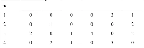
4. 4. 1. Positionchromosome This chromosome shows the scheduling of the use of the vehicles during the time horizon and the sequence of their movements per tour. This chromosome is a three-dimensional one with its rows as the number of the vehicles (v) and its columns as the number of the linehaul and backhaul customers (r + b). This matrix is repeated as much as the number of the periods of the planning horizon (t) and the entries of this chromosome show the "priority" of the services of each vehicle to the customers. For example, if the problem involves three linehaul customers, three backhaul customers, and four vehicles, and, for the first period, we reach the following numbers in the third row of the matrix, it means that, in this period, the third vehicle will respectively service the third and first linehaul customer and then the 6th and 4th backhaul customers. Besides, if no vehicle is used, all the entries in the row are zero (Table 1).
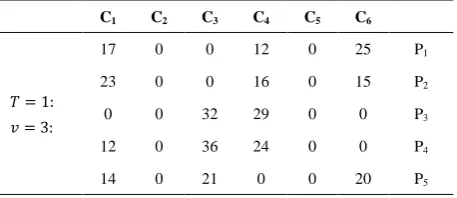
4. 4. 2. Distribution Chromosome This chromosome implies that after the assignation of the linehaul and backhaul customers to the vehicles in each period, how much of their demand for each product is met.
TABLE 1. Representation the Position Chromosome
𝒗
1 2 0
0 0
0 1
2 0 0
0 1
0 2
3 0 4
1 0
2 3
0 3 0
1 2
Since there is a possibility to split service of a customer between different vehicles, this matrix is four-dimensional. This matrix has rows according to the number of the products, i.e. p, columns according to the number of the customers. this matrix p * (r + b) is repeated as many times as the third dimension of the matrix, the vehicles (v), and the fourth dimension that is, the number of the periods in the time horizon (T). For example, if the distribution matrix is as follows (Table 2) for the first period and the third vehicle, it reveals that, in the first period, 17 units of the first type product, 23 units of the second type product, etc. has been shipped to the customer No. 1 by the vehicle No. 1. The same process is followed for all the other customers according to the priority given in the position chromosome. Various types of products are delivered to the customers’ No. 1 to 3, and received from the customers’ No. four to six.
4. 5. The Genetic Operators Based on the nature of the defined problem, in the crossover operator, for position chromosome the single-point method and for distribution chromosome arithmetic mean operator is used. Also in the mutation operator, for position chromosome, the swap operator and in the distribution chromosome, insertion operator is used.
4. 6. Feasibility Solution To be able to use the model, the repair process is used. In other words, each and every customer and vehicle should be checked considering the vehicle capacity, warehouse capacity, etc. For example, since that the stock out is not allowed, the load delivered to each linehaul customer and the inventory at the end of the previous period should not be less than his demand; and if this happens, then that customer should be deleted and placed in a file called “Assign” for reassignment.
4. 7. Algorithm Iteration After random generation of the initial population of the parents and the evaluation of them, the population of the children is created as much as the parents, according to the described selection method and genetic operators. Combining these two sets, the next generation is created according to the structure previously presented.
TABLE 2. Representation the Distribution Chromosome
C6
C5
C4
C3
C2
C1
P1 25 0 12 0 0 17
𝑇 = 1: 𝑣 = 3:
P2 15 0 16 0 0 23
P3 0 0 29 32 0 0
P4 0 0 24 36 0 12
P5 20 0 0 21 0 14
In this way, an iteration of the algorithm is performed, and so the process repeats until the final condition of the algorithm is established.
4. 8. Algorithm Stop Condition The most common condition is the frequency of the iterations of the algorithm, which is, for example, after the "n" iteration, the algorithm is stopped. In this model the same criterion is also considered.
5. COMPUTATIONAL RESULTS
In this paper, using several randomized test problems, the efficiency of the proposed genetic algorithm is evaluated with GAMS software. Theproposed genetic algorithm has been programmed and implemented in Matlab 8.6 environment. The stated algorithm is performed on a computer with Intel Core i3 processor,
64-bit, 1.7 GHz, Windows 7, and 4 GB of RAM.
5. 1. Creation of the Test Problems Given the variety of the constraints as well as the variables of the problem, with the enlargement of the dimensions, the complexity of the problem is greatly increased. The complex problems, due to the noticeable computational time and even insolubility of them by the exact methods, prevent the comparison of the algorithm with the exact GAMS method. Therefore, in this paper, small and almost average problems are used. Among of the most important parameters on the test problems are the number of the line-haul and backhaul customers, the variety of the products, the veracity of the vehicle capacity, the number of the periods in the planned horizons, and the other input parameters that are presented as follows (Table 3):
5. 2. Tuning of the Parameters In order to determine the genetic algorithm parameters, several experiments have been carried out with a set of different values of the parameters. Finally, using the following set of values, the best results are obtained (Table 4):
TABLE 3. Range for random generation of parameters
Range Parameter
Range Parameter
U [50, 500]
𝑑𝑖𝑗
U [20, 100]
𝑞𝑖𝑘𝑡
U [400, 1600]
𝑄𝑘
U [20, 100]
𝑅𝑖𝑘𝑡
U [500, 1200]
𝐶𝑖
U [10, 20]
𝑤𝑝
U [1500, 3500]
𝑓𝑘𝑡
U [150, 400]
ℎ𝑖𝑝
U [200, 500]
TABLE 4. GA parameters used for turning
Value GA Parameter
Row
0.7 Crossover Rate
1
0.3 Mutation Rate
2
150 Population Size
3
150 Iteration
4
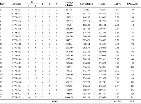
5. 3. NUMERICAL Results Each one of the test problems defined on the basis of the different parameters of the problem is applied 6 times by the proposed genetic algorithm and the best results obtained by the algorithm are presented in Table 5 along with the average of the obtained results. The attained answers are compared using the exact method (GAMS software) and the difference between the obtained fitness function is recorded by a comparison made by the application of the two methods. The average solution time of the genetic algorithm has been recorded for 150 iterations.
5. 4. Analysis of the Results According to the results represented in Table 5, it is observed that, in the
small size problems proposed for genetic algorithm, satisfactory responses were reached compared with the optimal solution showing a slight error rate. In general, the average error rate was about 3.415% in the random test problems. Figure 1 shows the comparison of the results of the above two methods. One of the most noticeable points considering the efficiency of the proposed algorithm is the solving time, while the computational time in the GAMS software increases exponentially with the increase in the dimensionality of the problem and it is almost impossible in the medium to high dimensions of the problem. Therefore, the necessity of using the meta-heuristic algorithms is significantly revealed.One of the most important analyzes that can be done,regarding the model developed in this study, is to compare the results of the model solution in the presence and absence of the division of the demand and the effect of that on the value of the target function and the cost variation of the model. Therefore, the model was first modeled in a non-split mode (no division of the demands), and a genetic algorithm was designed and coded to solve it.
TABLE 5. Comparison between GAMS and Proposed GA
Row Instance N T P V Average
solution Best Solution Gams GAP% 𝐂𝐏𝐔𝐭𝐢𝐦𝐞(𝒔)
R B
1 FTPS-n01 2 2 2 2 2 85186 81513 80290 1.5 20
2 FTPS-n02 2 2 4 4 3 153057 151117 148472 1.75 38
3 FTPS-n03 3 2 3 2 3 159395 146232 143000 2.21 36
4 FTPS-n04 2 3 4 3 3 212633 207915 203715 2.02 45
5 FTPS-n05 3 3 3 3 3 173754 156620 152141 2.86 42
6 FTPS-n06 3 3 4 2 4 224759 217724 209799 3.64 55
7 FTPS-n07 4 3 3 5 3 182669 124459 122356 1.69 54
8 FTPS-n08 4 4 4 4 3 311470 280443 266954 4.81 81
9 FTPS-n09 5 4 4 3 4 344392 325676 316850 2.71 75
10 FTPS-n10 5 5 5 2 4 389164 370564 354593 4.31 90
11 FTPS-n11 4 5 3 4 3 263990 253879 245044 3.48 56
12 FTPS-n12 6 4 3 4 4 259519 203358 193963 4.62 62
13 FTPS-n13 3 7 4 5 6 369210 334760 324081 3.19 130
14 FTPS-n14 8 3 3 3 5 302310 280238 273316 2.47 68
15 FTPS-n15 6 5 3 2 3 292460 284043 273477 3.72 53
16 FTPS-n16 6 6 4 4 4 504647 442235 423838 4.16 120
17 FTPS-n17 7 6 3 3 4 353775 342799 329361 3.92 85
18 FTPS-n18 9 5 5 5 5 825540 809936 774461 4.38 206
19 FTPS-n19 4 10 3 4 6 400884 334966 322973 3.58 89
20 FTPS-n20 11 5 4 6 6 657897 625770 601240 3.92 188
21 FTPS-n21 8 7 3 5 4 363255 282268 275663 2.34 129
22 FTPS-n22 6 9 4 7 6 752508 685605 650639 5.1 142
23 FTPS-n23 8 8 4 8 7 738836 712825 681389 4.41 239
24 FTPS-n24 10 7 5 6 6 1000201 988146 937059 5.17 261
Figure 1. Representation the results of Proposed GA and GAMS
Then, it was applied for all the random sample problems that were created in Table 5, and the results were presented in Table 6. It is important to note that the parameters of each sample problem (such as number of the customers, the number of the vehicles, types of the product, etc.) will definitely affect the obtained results. However, in general, the analysis of the results showed that 71% of the problems with the division of the demand has a lower cost than the ones with the absence of the division of the demand, and the average cost difference for all the sample problems is + 6.42%. In addition, in a segmentation, it was revealed thatin the problems concerning the number of the customers (Figures 2 and 3), (for the small problems with less than 10 customers) about 69% of the responses for the test problems with the split serviceshow better performance compared with the ones with non-split service (31%). In the problems containing 10 to 17 customers, this ratio ranged from 73% to 27%.
Then, all the above results indicate that the fitness function is optimized for a situation in which, in the problem, the division of demand is taken into consideration.
Figure 2. compare the results under 10 customers in split and without service mode
Figure 3. Compare the results for 10-17 customers in split and without service mode
TABLE6. Results obtained from split and without split service
Row Instance Best Solution GA with Split
Best Solution GA without
Split
GAP% Row Instance Best Solution GA with Split
Best Solution GA without
Split
GAP%
1 FTPS-n01 81513 97680 16.55 13 FTPS-n13 334760 357667 6.40
2 FTPS-n02 151117 195410 22.67 14 FTPS-n14 280238 294500 4.84
3 FTPS-n03 146232 150848 3.06 15 FTPS-n15 284043 224119 -26.74
4 FTPS-n04 207915 194366 -6.97 16 FTPS-n16 442235 498242 11.24
5 FTPS-n05 156620 160211 2.24 17 FTPS-n17 342799 267755 -28.03
6 FTPS-n06 217724 236202 7.82 18 FTPS-n18 809936 866355 6.51
7 FTPS-n07 124459 173702 28.35 19 FTPS-n19 334966 272519 -22.91
8 FTPS-n08 280443 250665 -11.88 20 FTPS-n20 625770 934805 33.06
9 FTPS-n09 325676 292929 -11.18 21 FTPS-n21 282268 427311 33.94
10 FTPS-n10 370564 347213 -6.73 22 FTPS-n22 685605 731405 6.28
11 FTPS-n11 253879 289667 12.35 23 FTPS-n23 712825 986719 27.76
12 FTPS-n12 203358 323981 37.23 24 FTPS-n24 988146 1076602 8.22
Average +6.42
0.00 10.00 20.00 30.00 40.00 50.00 60.00 70.00 80.00 90.00 100.00 110.00
1 3 5 7 9 11 13 15 17 19 21 23
C
o
st
(
S
ca
le
:
te
n
t
h
o
u
san
d
) GA GAMS
0.00 10.00 20.00 30.00 40.00
1 2 3 4 5 6 7 8 9 10 11 12 13
C
o
st
(
S
ca
le
:
te
n
t
h
o
u
san
d
)
With Split without Split
0.00 20.00 40.00 60.00 80.00 100.00 120.00
14 15 16 17 18 19 20 21 22 23 24
C
o
st
(
S
ca
le
:
te
n
t
h
o
u
san
d
6. CONCLUSION AND FUTURE RESEARCH
In the past two decades, companies and organizations have realized the importance of integrating the activities carried out in a supply chain and managing their processes efficiently. One of the major research areas in this area is optimizing the management of the supply and distribution of inventories in a supply chain, as an attempt to minimize the total cost of ordering, storing, and shipping the inventory. In this study, two operational features of routing problems, i.e. "backhauls" and "split service,” both of which are highly applicable to real world problems, are combined with the classical Inventory Routing Model. The outcome of this combination is expanded in the form of a model with multi-period and multi-product. The split service strategy was conducted based on the remaining capacity of the vehicles in each time period, while in backhauls, the service priority was given to linehaul clients.
In addition, the transportation fleet in the distribution network is heterogeneous. Due to the high computational complexity of the problem (NP-hardness), it was not possible to use the exact methods at the reasonable computational time, especially for large-scale problems. Therefore, an approximate solution method was introduced that was based on genetic algorithm, along with the problem solving in the small dimensions, by GAMS software. The efficiency of the proposed algorithm was evaluated using several random testing problems (up to 17 customers) (Table 5). The obtained results showed an average difference ratio of about 3.415%, when compared with the exact method. These findings manifest the proper performance of the proposed algorithm with an average solution time of approximately 98.5 seconds for 24 random testing problems. On the other hand, among the 24 testing problems (Table 6), about 70% of them had better answers in the case of the split service compared to the ones with no split. Given the accuracy of obtained results, future research can investigate issues such as the permissibility of stock outs and the inclusion of uncertainty in the demand of linehaul and backhaul customers in probability or dynamism modes. Also, the issue of production planning can be studied in order to expand the proposed model. Future studies that are concerned with solution methods, can also attempt to solve the proposed model with other new meta-heuristic algorithms to compare the results.
5. REFERENCES
1. Aghezzaf, E.-H., Raa, B. and Van Landeghem, H., "Modeling inventory routing problems in supply chains of high
consumption products", European Journal of Operational
Research, Vol. 169, No. 3, (2006), 1048-1063.
2. Prins, C., "A simple and effective evolutionary algorithm for the vehicle routing problem", Computers & Operations Research, Vol. 31, No. 12, (2004), 1985-2002.
3. Bell, W.J., Dalberto, L.M., Fisher, M.L., Greenfield, A.J., Jaikumar, R., Kedia, P., Mack, R.G. and Prutzman, P.J., "Improving the distribution of industrial gases with an on-line computerized routing and scheduling optimizer", Interfaces, Vol. 13, No. 6, (1983), 4-23.
4. Kleywegt, A.J., Nori, V.S. and Savelsbergh, M.W., "The stochastic inventory routing problem with direct deliveries",
Transportation Science, Vol. 36, No. 1, (2002), 94-118.
5. Andersson, H., Christiansen, M. and Fagerholt, K., Transportation planning and inventory management in the lng supply chain, in Energy, natural resources and environmental economics. 2010, Springer.427-439.
6. Coelho, L.C., Cordeau, J.-F. and Laporte, G., "Thirty years of inventory routing", Transportation Science, Vol. 48, No. 1, (2013), 1-19.
7. Coelho, L.C. and Laporte, G., "A branch-and-cut algorithm for the multi-product multi-vehicle inventory-routing problem",
International Journal of Production Research, Vol. 51, No. 23-24, (2013), 7156-7169.
8. Adulyasak, Y., Cordeau, J.-F. and Jans, R., "Formulations and branch-and-cut algorithms for multivehicle production and inventory routing problems", INFORMS Journal on
Computing, Vol. 26, No. 1, (2013), 103-120.
9. Coelho, L.C., Laporte, G. and Cordeau, J.-F., "Dynamic and stochastic inventory-routing, CIRRELT, (2012).
10. Santos, E., Ochi, L.S., Simonetti, L. and González, P.H., "A hybrid heuristic based on iterated local search for multivehicle inventory routing problem", Electronic Notes in Discrete
Mathematics, Vol. 52, (2016), 197-204.
11. Moin, N.H., Salhi, S. and Aziz, N., "An efficient hybrid genetic algorithm for the multi-product multi-period inventory routing problem", International Journal of Production Economics, Vol. 133, No. 1, (2011), 334-343.
12. Mjirda, A., Jarboui, B., Macedo, R., Hanafi, S. and Mladenović, N., "A two phase variable neighborhood search for the multi-product inventory routing problem", Computers & Operations
Research, Vol. 52, No., (2014), 291-299.
13. Sindhuchao, S., Romeijn, H.E., Akçali, E. and Boondiskulchok, R., "An integrated inventory-routing system for multi-item joint replenishment with limited vehicle capacity", Journal of Global
Optimization, Vol. 32, No. 1, (2005), 93-118.
14. Popović, D., Vidović, M. and Radivojević, G., "Variable neighborhood search heuristic for the inventory routing problem in fuel delivery", Expert Systems with Applications, Vol. 39, No. 18, (2012), 13390-13398.
15. Coelho, L.C. and Laporte, G., "The exact solution of several classes of inventory-routing problems", Computers &
Operations Research, Vol. 40, No. 2, (2013), 558-565.
16. Cordeau, J.-F., Laganà, D., Musmanno, R. and Vocaturo, F., "A decomposition-based heuristic for the multiple-product inventory-routing problem", Computers & Operations
Research, Vol. 55, (2015), 153-166.
17. Cárdenas-Barrón, L.E., González-Velarde, J.L. and Treviño-Garza, G., "A new approach to solve the product multi-period inventory lot sizing with supplier selection problem",
Computers & Operations Research, Vol. 64, (2015), 225-232.
with considering financial decisions", Journal of Industrial
Engineering and Management, Vol. 6, No. 4, (2013), 909-915.
19. Mirzaei, S. and Seifi, A., "Considering lost sale in inventory routing problems for perishable goods", Computers &
Industrial Engineering, Vol. 87, (2015), 213-227.
20. Azadeh, A., Elahi, S., Farahani, M.H. and Nasirian, B., "A genetic algorithm-taguchi based approach to inventory routing problem of a single perishable product with transshipment",
Computers & Industrial Engineering, Vol. 104, (2017), 124-133.
21. Moubed, M. and Mehrjerdi Zare, Y., "A hybrid dynamic programming for inventory routing problem in collaborative reverse supply chains", International Journal of Engineering,
TRANSACTIONS A: Basics, Vol. 29, No. 10, (2016),
1412-1420.
22. Liu, S.-C., Lu, M.-C. and Chung, C.-H., "A hybrid heuristic method for the periodic inventory routing problem", The
International Journal of Advanced Manufacturing
Technology, Vol. 85, No. 9-12, (2016), 2345-2352.
23. Fattahi, P., Tanhatalab, M. and Bashiri, M., "Bi-objectives approach for a multi-period two echelons perishable product inventory-routing problem with production and lateral transshipment", International Journal of
Engineering-Transactions C: Aspects, Vol. 30, No. 6, (2016), 876-882.
24. Yu, Y., Chen, H. and Chu, F., "Large scale inventory routing problem with split delivery: A new model and lagrangian relaxation approach", International Journal of Services
Operations and Informatics, Vol. 1, No. 3, (2006), 304-320.
25. Yu, Y., Chen, H. and Chu, F., "A new model and hybrid approach for large scale inventory routing problems", European Journal of Operational Research, Vol. 189, No. 3, (2008), 1022-1040.
26. Yu, Y., Chu, C., Chen, H. and Chu, F., "Large scale stochastic inventory routing problems with split delivery and service level constraints", Annals of Operations Research, Vol. 197, No. 1, (2012), 135-158.
27. Koza, J.R., "Genetic programming: On the programming of computers by means of natural selection, Cambridge, Mass., MIT Press, (1992).
Developing the Inventory Routing Problem with Backhauls, Heterogeneous Fleet and
Split Service
M. Forghani, M. A. Vahdat-Zad, A. Sadegheih
Department of Industrial Engineering, Faculty of Engineering, Yazd University, Yazd, Iran
P A P E R I N F O
Paper history: Received 30 July 2017
Received in revised form 08 January 2018 Accepted 15 February 2018
Keywords: Inventory-routing Backhauls Logistics Heterogeneous Fleet Split Delivery Genetic Algorithm Multi Product هديكچ یکی سب تاکن زا رای جنز رد مهم هری مأت ،نی يزاسلدم يانبمرب م هک نایرتشم فرصم نازی هب رجنم شهاک قلاشرثا یجنز ی هنیزهو هر ¬ لصاح ياه هیامرسزا ¬
لمحو يدوجوم رب يراذگ
¬ لقنو تلاوصحم دمآراک م ی ¬ ،دوش .تسا یگچراپکی نآ ¬ اه رد هلأسم یبایریسم -وم دوج ي کرت هک یبی ا ز دم تیری زوت عی دوجوم و ي م ی ¬ ،دشاب من دو پ ادی م ی ¬ دنک ا . نی هلاقم کی کرت بی لمع یتای سم هلأسم زا یبایری -وم دوج ي سلاک کی ب ژتارتسا ا ي
ط رد لاسرا ی سم ری و یکی و زا یگژی ¬ ياه سب رای اسم مهم لی سم یبایری ینعی " تشگزابرد لمح " ولوا( تی تمدخ ¬ یناسر هب م رتش نای خ ط
لماش قوف لدم .تسا هداد طسب )تفر کی دنچ هلأسم -رپ ،يدوی چ دن -،یلوصحم سودنچ هلی ¬ يا ا ارب و هدوبن زاجم دوبمک هک تس ي
سا هدافت
فرظ زا رتهب تی اسو هدافتسالاب لی لقن هی و زا یگژی « سقت می اضاقت » ا ،قوف تاضورفم هب هجوت اب .تسا هدش هدافتسا أسم ادتب
تروص هب هل ی ک رلدم یضای حص ددع حی زاسلدمطلتخم ي لد هب و هدش لی ا هکنی اسم هرمز رد لی پ اب ی چ یگدی ،دراد رارق تخس کی روگلا متی ف کتباار را ي « تنژ کی اراک » ارب ي رشت نآ لح حی اپ رد .تسا هدش نای
لحتهب ابمتیروگلانیازلاصاحیددعجیاتنلی اسم زا هدافتسا
لی اصت هنومن فد ی رپ و هدشهتخاد ن ات جی ب رگنای شهاک 70 دصرد ي زه هنی ¬ اه ژتارتسا زا هدافتسا اب ي
سقت می .تسا هدوب اضاقت
doi: 10.5829/ije.2018.31.06c.12