Optimization of Closed-Loop Supply Chain Problem for Calculation Logistics Cost Accounting

Published online January 28, 2015 (http://www.sciencepublishinggroup.com/j/ijiis) doi: 10.11648/j.ijiis.s.2015040201.11

ISSN: 2328-7675 (Print); ISSN: 2328-7683 (Online)

Optimization of closed-loop supply chain problem for

calculation logistics cost accounting

Lee Jeongeun, Rhee Kyonggu

Department of Accounting, Dongeui University, Busan, Korea

Email address:

[email protected] (Lee J.), [email protected] (Rhee K.)

To cite this article:

Lee Jeongeun, Rhee Kyonggu. Optimization of Closed-Loop Supply Chain Problem for Calculation Logistics Cost Accounting. International Journal of Intelligent Information Systems. Special Issue: Logistics Optimization Using Evolutionary Computation Techniques.

Vol. 4, No. 2-1, 2015, pp. 1-6. doi: 10.11648/j.ijiis.s.2015040201.11

Abstract:

This paper aims to build closed loop supply chain model (CLSCM) and propose a multi-objective genetic algorithm. This paper designs the method of calculation for a solution using optimization algorithms with the priority-based genetic algorithm (priGA), and Adaptive Weight Approach (AWA).In this paper, we present a multi-objective closed loop supply chain model in integrated logistics system. We formulated a mathematical model with two objectives functions: (1) minimize transportation cost, open cost, inventory cost, purchase cost, disposal cost and saving cost of integrated facilitiesof CLSCM, (2) minimize the delivery time tardiness in all periods. Finally, a simulation is investigated to demonstrate the applicability of the proposed multi-objective closed loop supply chain model (CLSCM) and solution approaches.

Keywords:

Closed-Loop Supply Chain, Logistics Cost Accounting, Genetic Algorithm

1. Introduction

Reverse Logistics, which is the logistics activity covering over the produce recovery, recycling, waste disposal and etc., has received considerable attention due to the following two reasons. First, the seriousness of environmental problem has been embossed in corporate logistics activity and the environmental logistics problem has been international issue by Government Resolutions and etc. Second, the resources have been exhausted all over the world.

In the recent years due to the ever-increasing development of the competitive environment, the researchers have paid attention to the supply chain network problem. This problem has a key importance role in long-term decisions/performance and requires to be optimized for efficiency of the whole supply chain [1].

In the following, we introduce research papers associated with closed-loop supply chain model (CLSCM).

Ma and Wang [2] consider a closed-loop supply chain (CLSC) with product recovery, which is composed of one manufacturer and one retailer. The retailer is in charge of recollecting and the manufacturer is responsible for product recovery. The system can be regarded as a coupling dynamics of the forward and reverse supply chain.

Chuang et al. [3] study closed-loop supply chain models

for a high-tech product which is featured with a short life-cycle and volatile demand. They focus on the manufacturer's choice of three alternative reverse channel structures (i.e., manufacturer collecting, retailer collecting, and third-party firm collecting) for collecting the used product from consumers for remanufacturing: (1) the manufacturer collects the used product directly; (2) the retailer collects the used product for the manufacturer; and (3) the manufacturer sub contracts the used product collection to a third-party firm.

Lee et al. [4] is also proposed multi-objective closed-loop supply chain model. However, they only consider a limited logistics cost (e.g., transportation cost and open cost). We propose the improved model considering minimization of total cost (e.g., transportation cost, open cost, inventory cost, purchase cost, disposal cost and saving cost of integrated facilities)and minimization of total delivery tardiness.

2. Problem Definition

2.1. Mathematical Model of CLSC

The model is a multi-objective problem considered the multi echelon, multi period, and multi product in closed-loop supply chain. We formulated the CLSCM as a multi-objective 0-1 mixed integer linear programming model.

The following assumptions are made in the development of the model:

A1. Only one product is treated in closed loop supply chain model.

A2. The inventory factor is existed over finite planning horizons.

A3. The requirement by manufacturer and the quantity of collected products is known in advanced.

A4. The maximum capacities about echelons are known. A5. All of inventory holding costs of processing centers are same.

A6. In the case of transportation from processing center to manufacturer, the lot size is 100 and the lead time is not considered.

The parameters, decision variables, objective functions, and restrictions in this closed-loop supply chain model are as follows.

(1) Indices

i index of manufacturer (i=1,2,…, I) j index of distribution center (j=1,2,…, J) k index of retailer (k=1,2,…, K)

l index of customer (l=1,2,…, L)

k` index for returning center (k`=1,2,…, K`) m index of processing center (m=1,2,…, M) t index of time period (t=1,2,…, T) (2) Parameters

I number of manufacturers J number of distribution centers K number of retailers

L number of customers K` number of returning centers M number of processing centers N disposal center

S supplier

T planning horizons

ai capacity of manufacturer i

bj capacity of distribution center j

u capacity of retailer k uk` capacity of returning center k`

um capacity of processing center m

di demand of manufacturer i

c1ij unit cost of transportation from manufacturer i to

distribution center j

c2jk unit cost of transportation from distribution center j to

retailer k

c3kl unit cost of transportation from retailer k to customer l

c4lk` unit cost of transportation from customer l to returning

center k`

c5k`m unit cost of transportation from returning center k` to

processing center m

c6Mn unit cost of transportation from processing center m to

disposal N

c7mi unit cost of transportation from processing center m to

manufacturer i

c8Si unit cost of transportation from supplier S to

manufacturer i

cOj open cost of distribution center j

cOk open cost of retailer k

cOk` open cost of returning center k`

cH j unit holding cost of inventory per period at distribution

center j

cHk unit holding cost of inventory per period at retailer k

cHk` unit holding cost of inventory per period at returning

center k`

cHm unit holding cost of inventory per period at processing

center m

rN disposal rate

dij delivery time from returning center i to processing

center j

djM delivery time from processing center j to manufacturer

M

pj processing time for reusable product in processing

center j

tE expected delivery time by customers

(3) Decision variables

x1ij(t) amount shipped from manufacturer i to distribution

center j in period t

x2jk(t) amount shipped from distribution center j to retailer

k in period t

x3kl(t) amount shipped from retailer k to customer l in

period t

x4ik`(t) amount shipped from customer l to returning center

k` in period t

x5k`m(t) amount shipped from returning center k` to

processing center m in period t

x6mN(t) amount shipped from processing center m to

disposal N in period t

x7mi(t) amount shipped from processing center m to

manufacturer i in period t

x8Si(t) amount shipped from supplier S to manufacturer i

in period t

yj(t) inventory amount at distribution center j in period t

yk(t) inventory amount at retailer k in period t

yk`(t) inventory amount at returning center k` in period t

ym(t) inventory amount at processing center m in period t

2.2. Mathematical Formulation

The first objective function, f1 consists of the total cost.

Minimize {f1,f2} (1)

Min

f1=TC + OC + IC + PC + RTC + ROC + RIC + DC – SC (1) a

The cost components in the objective function F1 can be

1 1 2 2 3 3

1 1 1 1 1 1

TC ( ) ( ) ( )

I J J K K L

ij ij jk jk kl kl

i j j k k l

c x t c x t c x t

= = = = = =

 

= + + 



∑∑

∑∑

∑∑



Forward logistics open costs

O O

1 1

OC ( ) ( )

J K

j j k k

j k

c z t c z t

= =

=

∑

+

∑

Forward logistics inventory costs

H H

1 1 1 1

IC ( ) ( )

J K K L

j j k k

j k k l

c y t c y t

= = = =

=

∑∑

+

∑∑

Forward logistics purchase costs

8 8

1

PC ( )

I

Si Si i

c x t =

=

∑

Reverse logistics transportation costs

` `

4 4 5 5 7 7

` ` ` `

1 ` 1 ` 1 1 1 1

RTC ( ) ( ) ( )

L K K M M I

lk lk k m k m mi mi

l k k m m i

c x t c x t c x t

= = = = = =

=

∑∑

+

∑∑

+

∑∑

Reverse logistics open costs

'

' ' ' 1

ROC ( )

K O k k k

c z t =

=

∑

Reverse logistics inventory costs

`

H H

` `

` 1 1 1 1

RIC ( ) ( )

K M M I

k k m m

k m m i

c y t c y t

= = = =

=

∑∑

+

∑∑

Reverse logistics disposal costs

6 6

1

DC ( )

M

mN mN m

c x t =

=

∑

Saving cost from integrating retailer/returning center

` O

` 1 ` 1

SC ( ) ( )

K K

k k k

k k

c z t z t = =

=

∑∑

The second objective function, f2 is total delivery

tardiness. min f2

2

0 1 1 1

( ) ( ) ( ) ( )

T I J J

ij ij jM j jM E M

t i j j

f d x t d p x t t d t

= = = =

 

=  + + −

 

∑ ∑∑

∑

(1)b

Subject to - open cost

1−z t_j( − =1) z t_j( ) ∀ ∈j J t, ∈T (2)

1−z t_k( − =1) z t_k( ) ∀ ∈k K t, ∈T (3)

- inventory costs

1 2

( ) ( ) ( 1) ,

j ij jk

y t =x t +x t− ∀ ∈j J t∈T (4)

2 3 4 5

` ` `

( ) ( ) ( ) ( 1) ( ) ( 1)

, ` `,

k k jk kl ik k m

y t y t x t x t x t x t

k K k K t T

+ = + − + + −

∀ ∈ ∈ ∈ (5)

5 7 6

`

( ) ( ) ( 1) ( ) ,

m k m mi mN

y t =x t +x t− − x t ∀ ∈m M t∈T (6)

- disposal costs

`

6 5

`

1 ` 1 1

( ) ( )

M K M

mN k m N

m k m

x t x t r t T

= = = = ∀ ∈

∑

∑∑

(7)

- capacity constraints

1 1 ( ) , J ij i j

x t a i I t T

=

≤ ∀ ∈ ∈

∑

(8)

2

1

( ) ( 1) ( ) ,

K

jk j j j

k

x t y t b z t j J t T

=

+ − ≤ ∀ ∈ ∈

∑

(9)

3 5

` ` ` `

1 1

( ) ( 1) ( ) ( 1) ( ) ( )

, ` `,

L M

kl k k m k k k k k

l m

x t y t x t y t u z t u z t

k K k K t T

= =

+ − + + − ≤ +

∀ ∈ ∈ ∈

∑

∑

(10)

- demand constraints

7 8 1

( ) ( ) ( )

mi Si ij i

x t +x t +x t =d ∀ ∈t T (11)

1

( ) ( ),

J

jM M j

x t d t t

= ≤ ∀

∑

(12)

- non-negativity constraints

1 2 3 4 5 6 7 8

` `

( ), ( ), ( ), ( ), ( ), ( ), ( ), ( ) 0

,

ij jk ij lk k m mN mi Si

x t x t x t x t x t x t x t x t

i I, j J, k K, l L, m M t T

≥

∀ ∈ ∈ ∈ ∈ ∈ ∈ (13)

- binary constraints

{ }

( ) 0,1 ,

j

z t = ∀ ∈j J t∈T (14)

{ }

( ) 0,1 ,

k

z t = ∀ ∈k K t∈T (15)

{ }

`( ) 0,1 ` `,

k

z t = ∀ ∈k K t∈T (16)

H 1

( ) ( 1) , ,

I

ij j j j i

x t y t b z j t

=

+ − ≤ ∀

∑

(17)

H H

1

( 1) ( ) ( ) ( ),

I

j ij jM j i

y t x t x t y t j, t =

− +

∑

− = ∀ (18)

H

( ), ( ), ( ) 0, ,

ij jM j

x t x t y t ≥ ∀i j, t (19)

3. Optimization of the Closed-Loop

Supply Chain with the Genetic

Algorithm

3.1. Priority-Based Encoding Method

and its length is equal to total number of sources m and depots n, i.e. m+n. The transportation tree corresponding with a given chromosome is generated by sequential arc appending between sources and depots [5]. At each step, only one arc is added to tree selecting a source (depot) with the highest priority and connecting it to a depot (source) considering minimum cost [6].

3.2. Adaptive Weight Approach

While we consider multiobjective problem, a key issue is to determine the weight of each objective. Gen et al.[7] proposed an Adaptive Weight Approach (AWA) that utilizes some useful information from the current population to readjust weights for obtaining a search pressure toward a positive ideal point[8]. In this study, we are using the following objectives:

(1) Minimization of the total cost (cT)

(2) Minimization of the delivery tardiness. (cD)

1 2

1 T 2 D

1 1 1 1

max {f , }

( )

k k

f

f (v ) c f v c

= = = = (20)

For the solutions at each generation, zqmax and zqmin are the

maximal and minimal values for the qth objective as defined by the following equations:

max

min

max{ ( ), 1, 2, ... , }, 1,2 min{ ( ), 1, 2, ... , }, 1,2

q q k

q q k

z f v k popSize q

z f v k popSize q

= = =

= = = (21)

The adaptive weights are calculated as

max min

1

, 1,2

q

q q

w q

z z

= =

− (22)

The weighted-sum objective function for a given chromosome is then given by the following equation

2

min 1

( )k q( q( )k q ), 1,2,...

q

eval v w f v z k , popSize =

=

∑

− = (23)

4. Simulation

In this section, multiobjective hybrid genetic algorithm and CPLEX software is used to compare the results of small-size problems. All the test problems are solved on a Pentium 4, 3.20GHz clock pulse with 1GB memory. The data in test problems were also randomly generated to provide realistic scenarios.The 3 test problems were combined, as shown in Table 1.

Table 1. The size of test problems (Rhee et al. [9])

Problem No. Period returning centers(I) processing centers(J) No. of constraints No. of variables

1 4 5 3 264 120

2 4 10 6 852 404

3 4 20 15 2988 1452

We ran the procedure for 20 times for each problem considering following parameters:

Population size, popSize=100;

Maximum generations, maxGen=1000; Crossover probability, pC=0.7;

Mutation probability, pM=0.3

4.1. Numerical Results

In this paper, we compared percentage gap of CPLEX, Priority-based encoding method with Adaptive Weight Approach (pri-awGA) and multiobjective hybrid genetic algorithm (mo-hGA).

In order to compare the non-dominated solutions of the two methods, the value of the second objective function (f2) of

each solution obtained by mo-hGA is insesrted into the model formulation as a new constraint.

gap(%)=100(GA f1- CPLEX f1)/ CPLEX f1 (24)

In table 2, we explain the simulation results for 3 test problems with 20 instances in each. We use the percentage gap between optimum solution and heuristic solutions, which are pri-awGA and mo-hGA. And we also compare CPLEX f1 and

GAs f1 and Pareto solutions (f1, f2) at the same time.

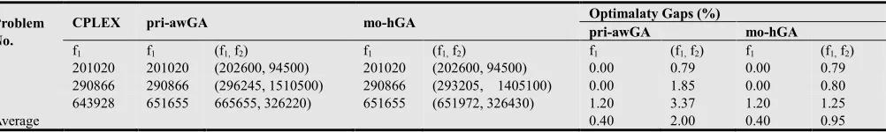
Table 2. The comparison of CPLEX, pri-awGA and mo-hGA with Optimality Gaps

Problem No.

CPLEX pri-awGA mo-hGA Optimalaty Gaps (%)

pri-awGA mo-hGA

f1 f1 (f1, f2) f1 (f1, f2) f1 (f1, f2) f1 (f1, f2)

1 201020 201020 (202600, 94500) 201020 (202600, 94500) 0.00 0.79 0.00 0.79

2 290866 290866 (296245, 1510500) 290866 (293205, 1405100) 0.00 1.85 0.00 0.80

3 643928 651655 665655, 326220) 651655 (651972, 326430) 1.20 3.37 1.20 1.25

Average 0.40 2.00 0.40 0.95

When the GAs f1 are compared with respect to average gap

over all 3 problems, the result are same CPLEX, pri-awGA and mo-hGA in problem 1 and 2. On the other hand, the average gap in pri-awGA and mo-hGA are 1.20% over CPLEX in problem 3.

When the Pareto solutions (f1, f2) are compared with respect

The comparison is first done according to the computation time and it is seen that the computation time needed for mo-hGA is less than pri-awGA in all problems. Next, according to the number of Pareto solutions, both methods found the same number for problem 1, and they are slightly same for problem 2. But for problem 3, the number of Pareto

solutions found by pri-awGA are less than that found by mo-hGA. Finally the improvement rate according to each time period are shown in the last column of Table 3. When comparing number of Pareto solutions, the results are same in problem 1 and 2. On the other hand, the result using mo-hGA is better in problem 3.

Table 3. The experimental results of pri-awGA and mo-hGA

No. Time

period

Computational time[sec] No. of Pareto solutions [Sj]

pri-awGA mo-hGA Improvement Rate(%) pri-awGA mo-hGA Improvement Rate(%)

1

t=1

4,537 3,546 21.84

3 3 0.00

t=2 5 5 0.00

t=3 2 2 0.00

t=4 4 4 0.00

2

t=1

4,596 3,596 21.76

5 6 20.00

t=2 7 7 16.67

t=3 6 8 33.33

t=4 9 8 -11.11

3

t=1

4,646 3,656 21.31

7 13 85.71

t=2 6 9 50.00

t=3 6 10 66.67

t=4 8 9 12.50

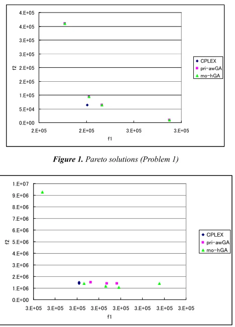
Fig. 1~3 represents Pareto solutions obtained from CPLEX, pri-awGA and mo-hGA for test problems. In this figure, the corresponding solutions on CPLEX and pri-awGA and mo-hGA Pareto optimal solutions with the same f2 values are

labeled with the same letters.

0 .E+0 0 5 .E+0 4 1 .E+0 5 2 .E+0 5 2 .E+0 5 3 .E+0 5 3 .E+0 5 4 .E+0 5 4 .E+0 5

2 .E+ 0 5 2 .E+ 0 5 3 .E+ 0 5 3 .E+ 0 5 f 1

f

2

CPLEX pri- awGA mo- h GA

Figure 1. Pareto solutions (Problem 1)

0 .E+ 00 1 .E+ 06 2 .E+ 06 3 .E+ 06 4 .E+ 06 5 .E+ 06 6 .E+ 06 7 .E+ 06 8 .E+ 06 9 .E+ 06 1 .E+ 07

3 .E+ 05 3.E+0 5 3 .E+ 0 5 3.E+0 5 3 .E+ 0 5 3 .E+ 05 3.E+0 5 3 .E+ 05 f 1

f

2

CPLEX pri- awGA mo- hGA

Figure 2. Pareto solutions (Problem 2)

3 .2 4 E+ 0 5 3 .2 6 E+ 0 5 3 .2 8 E+ 0 5 3 .3 0 E+ 0 5 3 .3 2 E+ 0 5 3 .3 4 E+ 0 5

6 .E+ 0 5 6 .E+ 0 5 6 .E+ 0 5 7 .E+ 0 5 7 .E+ 0 5 7 .E+ 0 5 7 .E+ 0 5 f 1

f

2

CPLEX pri- awGA mo- h GA

Figure 3. Pareto solutions (Problem 3)

5. Conclusion

In this paper, we presented 0-1 mixed-integer linear programming model for multi-objective optimization of CLSCM and a genetic algorithm approach.

We propose the improved model considering minimization of total cost (e.g., transportation cost, open cost, inventory cost, purchase cost, disposal cost and saving cost of integrated facilities) and minimization of total delivery tardiness.

Finally, through the comparison of percentage gap of CPLEX, Adaptive Weight Approach (pri-awGA) and multi-objective hybrid genetic algorithm (mo-hGA), the effectiveness of the proposed method was demonstrated.

References

[2] Junhai Ma, Hongwu Wang, “Complexity analysis of dynamic noncooperative game models for closed-loop supply chain with product recovery”, Applied Mathematical Modelling, Vol. 38, No. 23, 2014, pp. 5562–5572.

[3] Chia-Hung Chuang, CharlesX.Wang , YabingZhao, “Closed-loop supply chain models for a high-tech product under alternative reverse channel and collection cost structure”s, International Journal of Production Economics, Vol. 156, 2014, pp. 108-123.

[4] Lee, J. E. Chung, K. Y., Lee, K. D. and Gen, M., “A multi-objective hybrid genetic algorithm to minimize the total cost and delivery tardiness in a reverse logistics”, Multimedia Tools and Applications, published online, 03 August 2013. [5] Syarilf, A. and Gen, M., “Double Spanning Tree-based Genetic

algorithm For Two Stage Transportation Problem”,

International Journal of Knowledge-Based Intelligent Engineering System, Vol. 7, No. 4, 2003, pp. 388-389. [6] Gen, M. and Cheng, R., Genetic Algorithms and Engineering

Optimization, John Wiley and Sons, New York, 2000. [7] Gen, M., Cheng, R. and Lin, L., Network Models and

Optimization: Multiobjective Genetic Algorithm Approach, Springer, 2008.

[8] Altiparmak, F., Gen, M., Lin, L. and Paksoy, T., “A genetic algorithm approach for multi-objective optimization of supply chain networks”, Computers & Industrial Engineering, Vol. 51, No. 1, 2006, pp. 197-216.