Task Clustering and Gating for Bayesian Multitask Learning
Bart Bakker [email protected]
Tom Heskes [email protected]
SNN, University of Nijmegen Geert Grooteplein 21
6525 EZ Nijmegen, The Netherlands
Editor: Michael I. Jordan
Abstract
Modeling a collection of similar regression or classification tasks can be improved by making the tasks ‘learn from each other’. In machine learning, this subject is approached through ‘multitask learning’, where parallel tasks are modeled as multiple outputs of the same network. In multilevel analysis this is generally implemented through the mixed-effects linear model where a distinction is made between ‘fixed effects’, which are the same for all tasks, and ‘random effects’, which may vary between tasks. In the present article we will adopt a Bayesian approach in which some of the model parameters are shared (the same for all tasks) and others more loosely connected through a joint prior distribution that can be learned from the data. We seek in this way to combine the best parts of both the statistical multilevel approach and the neural network machinery.
The standard assumption expressed in both approaches is that each task can learn equally well from any other task. In this article we extend the model by allowing more differentiation in the similarities between tasks. One such extension is to make the prior mean depend on higher-level task characteristics. More unsu-pervised clustering of tasks is obtained if we go from a single Gaussian prior to a mixture of Gaussians. This can be further generalized to a mixture of experts architecture with the gates depending on task characteristics. All three extensions are demonstrated through application both on an artificial data set and on two real-world problems, one a school problem and the other involving single-copy newspaper sales.
Keywords: Empirical Bayes; Multitask learning; Mixture of experts; Multilevel analysis.
1. Introduction
Many real-world problems can be seen as a series of similar, yet self contained tasks. Examples are the school problems (see e.g. Aitkin and Longford, 1986), and clinical trials. The first example deals with the prediction of student test results for a collection of schools, based on school demographics. The similar tasks in the other example can be the prediction of survival of patients in different clinics (see e.g. Daniels and Gatsonis, 1999). The relatedness (and therefore interdependency) of such models is taken into account and benefitted from in the fields of multitask learning (or learning to learn) and ‘multilevel analysis’. In the present article we seek to combine insights that are obtained in the multilevel field with methods that have been designed in the neural network community to create a synergetic new approach.
Multilevel analysis is generally based on the ‘mixed-effects linear model’. This model features a response that is made up from the sum of a fixed effect and a random effect. The fixed effect implements a ‘hard sharing’ of parameters, whereas the random effect implies a ‘soft sharing’ through the use of a common distribution for certain model parameters. A more elaborate description of multilevel analysis is given in Section 6. A neural network model would use ‘hard shared’ parameters (the same for each of the parallel tasks) to detect ‘features’ in the covariates x, and use these features for regression (Baxter, 1997, Caruana, 1997). Feature detection can be implemented, for example, in the hidden layers of a multi-layered perceptron, or through principal component analysis. This use of features is appropriate when the covariates are relatively high-dimensional, as they are for the real-world problems addressed in the present article.
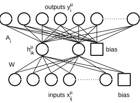
inputs xijµ bias W
hikµ bias
A i
outputs yiµ
Figure 1: Neural network model. The input-to-hidden weights W are shared by (equal for) all tasks. Each of the outputs (top layer) represents one task, and has its own set of task-dependent hidden-to-output weights Ai.
optimization has previously been studied by Baxter (1997): he showed that the risk of overfitting the shared parameters is an order N (the number of tasks) smaller than overfitting the task-specific parameters (hidden-to-output weights). The remaining parameters specific to each task are treated in a Bayesian manner. In the multitask setting, where data from all tasks can be used to fit the shared parameters, this empirical Bayesian approach is a natural choice and a close approximation to a full Bayesian treatment.
Any multitask learning model makes use of the fact that the tasks (the parallel sets of responses and covariates) are somehow related. Although for particular sets of tasks the nature of this relationship may be immediately clear, on other occasions more subtle relations may exist. Even if all tasks in a set are related, some may be stronger related to each other than to others. We accommodate for this possibility by suggesting a form of ‘task clustering’ (Section 4). Allowing a fixed number of task clusters we are able to obtain better estimates for the responses y, and discern hidden structure within the set of tasks.
We will describe the general structure of the multitask learning model in Section 2. We present our Bayesian treatment of multitask learning and knowledge sharing in Section 3, and show how to optimize the shared parameters of the model. In Section 4 we extend the method so that it may allow a distinction between (groups of) tasks. The model is tested (Section 5) both on an artificial data set, which consists of samples drawn from a mixture of Gaussians, and on two real-world data sets: the Junior School Problem (predicting test results for British school children) and the Telegraaf problem (predicting newspaper sales in The Netherlands). We show that the method presented in this article yields both better predictions and a meaningful clustering of the data. Section 6 describes the links of the present article with related work. We finish with concluding remarks and an outlook on future work in Section 7.
2. A Neural Network Model
Suppose that for task i we are given a data set Di={xµi,y µ
i}, with µ=1...ni, the number of examples for task i. For notational convenience, we assume that the response yµi is one-dimensional. The input xµi is an
ninput-dimensional vector with components xµik. Our model assumption is that the response yµi is the output of a multi-layered perceptron with additional Gaussian noise of standard deviationσ(see also Figure 1). Each output unit represents the response for one task.
In our model, the input-to-hidden weights W are shared by (equal for) all tasks, whereas the hidden-to-output weights are task-dependent (see Figure 1). In this format the expression for the response yµi reads:
yµi =
nhidden
∑
j=1
Ai jhµi j+Ai0+noise, hµi j=g ninput
∑
k=1
Wjkxµik+Wj0 !
, (1)
with W the nhidden×(ninput+1)matrix of input-to-hidden weights (including bias) and Ai an(nhidden+1) -dimensional vector of hidden-to-output weights (and bias). The extra index i in the hidden unit activity hµi follows from the dependency of the covariates xµi on task i. For notational simplicity we will include hµi0=1 in hµi and Ai0in Aifrom now on.
3. Computation and Optimization
Let us now consider the full set of tasks, for which we define the complete data set D={Di}, with i=1...N,
the number of tasks. For notational convenience we will assume all inputs xµi fixed and given and omit them from our notation. A denotes the full N×(nhidden+1)-dimensional matrix of hidden-to-output weights. Note that these are specific for each task, whereas all other parameters are shared between tasks. We assume the tasks to be iid given the hyperparameters, and define a prior distribution for the task-dependent parameters:
Ai∼
N
(Ai|m,Σ), (2)which is a Gaussian with an(nhidden+1)-dimensional mean m and an(nhidden+1)×(nhidden+1)covariance matrixΣ.
This prior distribution is incorporated into the posterior probability of data and hidden-to-output weights given the hyperparametersΛ={W,m,Σ,σ}. The joint distribution of data and model parameters reads
P(D,A|Λ) =
N
∏
i=1
P(Di|Ai,W,σ)P(Ai|m,Σ),
where we used the assumption that the tasks are iid givenΛ.
Integrating over A we obtain, after some calculations (see Appendix A for details)
P(D|Λ) =
N
∏
i=1
P(Di|Λ),
with
P(Di|Λ)∝
|Σ|σ2ni|Qi|
−1 2
exp
1 2(R
T
iQ−i1Ri−Si)
, (3)
where Qi, Riand Siare functions of DiandΛgiven by
Qi = σ−2 ni
∑
µ=1
hµihµiT+Σ−1, Ri=σ−2 ni
∑
µ=1
yµihµi+Σ−1m,
Si = σ−2 ni
∑
µ=1
yµi2+mTΣ−1m. (4)
(Recall that hµi depends on W and xµi.) Optimal parametersΛ∗are now computed by maximizing the like-lihood (3). This is referred to as empirical Bayes (Robert, 1994), and is similar to MacKay’s evidence framework (MacKay, 1995). Here it is motivated by the fact that we can use the data of all tasks to optimize
numbers of tasks, Baxter (1997) shows that the generalization error as a function of the number of tasks N and the dimension of the hyperparameters|Λ|is proportional to|Λ|and inversely proportional to N (see also Heskes, 2000).
Given the maximum likelihood parametersΛ∗, we can easily compute P(Ai|Di,Λ∗)to make predictions, compute error bars, and so on. The parameter
˜
Ai=argmax
Ai
P(Ai|Di,Λ∗)
will be referred to as the maximum a posteriori orMAPvalue for Ai.
When g(·)in (1) is a linear function, we can simplify Equation 3 significantly (see Appendix A). This gives us the advantage that instead of using the full data sets Di={xµi,y
µ
i}for each task, we only need the sufficient statisticsxixTi
,hxiyiiand
y2ifor optimization, whereh..idenotes the average over all examples
µ.
4. Making Some Tasks More Similar Than Others
The prior (2) may be useful when we have reason to believe that a priori all tasks are ‘equally similar’. In many applications, this assumption is a little too simplistic and we have to consider more sophisticated priors. 4.1 Task-dependent Prior Mean
We can make the prior distribution task-dependent by introducing higher-level task characteristics, that is, ‘features’ of the task that are known beforehand. We will denote them fifor task i. These features, although they have different values for different tasks, do not vary within one task. Therefore, rather than adding them as extra inputs, we use these features to make the prior mean task-dependent. A straightforward way to include these features into the prior mean is to make it a linear function of these features, that is,
mi=Mfi,
with M now an(nhidden+1)×nfeaturematrix. We are back to the independent prior mean if we take nfeature=1 and all fi=1.
The calculation of the likelihood proceeds as in Section 3, with m in (4) replaced by mi. With a linear form optimization is hardly more involved, but in principle we can take more complicated nonlinear dependencies into account as well.
4.2 Clustering of Tasks
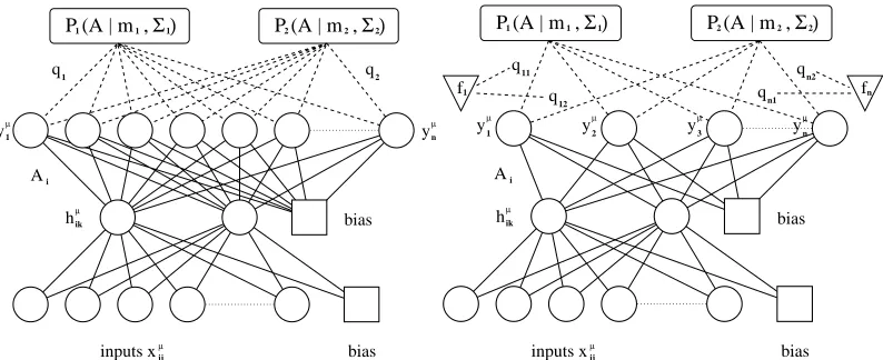
Another reasonable assumption might be that we have several clusters of similar tasks instead of a single cluster. Then we could take as a prior a mixture of nclusterGaussians,
Ai∼ ncluster
∑
α=1
qα
N
(mα,Σα) (5)instead of the single Gaussian (2). Each Gaussian in this mixture can be seen to describe one ‘cluster’ of tasks. In Equation 5, qαrepresents the a priori probability for any task to be ‘assigned to’ clusterα(see also Figure 2). Although a priori we still do not distinguish between different tasks, a posteriori tasks can be assigned to different clusters. The posterior data likelihood reads:
P(Di|Λ) =
Z
dAiP(Di|Ai,Λ) ncluster
∑
α=1
qαP(Ai|mα,Σα). (6)
P (A | m , Σ ) q1 Ai hik µ q 1 1
1 2 2 2
P (A | m , Σ )
2
inputs xij
µ bias bias µ y1 µ yn
P (A | m , Σ )
Ai f1 11 q 1 1
1 2 2 2
P (A | m , Σ )
inputs xij
µ bias bias q q q 12 n1 n2 fn
y1 y2 y3 yn
hik µ
µ µ µ µ
Figure 2: The task clustering (left) and task gating model (right). In task clustering the task-dependent weights Ai are supposed to be drawn from a weighted sum of Gaussians, where the weights qα are equal for all tasks. In task gating these weights become task-dependent and the value for qiα depends on the task-specific feature vector fi.
this way, the posterior distribution effectively ‘assigns’ tasks to that cluster that is most compatible with the data within the task, in the sense that all other clusters (Gaussians) do contribute much less to (6).
We introduce indicator variables ziα where ziα equals one if task i is assigned to cluster α and zero otherwise. For any task i only one ziαmay be one. To optimize the likelihood of the shared parametersΛ, which now include all cluster means and covariances as well as the prior assignment probabilities q, we can apply an expectation-maximization or EM-algorithm (see e.g. Dempster et al., 1977).
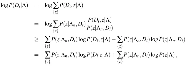
If the cluster assignments ziα were known, optimization of log P(D,z|Λ)with respect to Λ would be relatively simple. The values for ziα however are not known, so in the E-step we estimate the expectation value of log P(D,z|Λ)under P(z|D,Λn), where forΛnwe take the current values forΛ(which are initialized randomly at the start of the procedure). In the M-step the obtained expectation value is maximized forΛ. This step is of roughly the same complexity as the optimization for a single cluster. Both steps are repeated untilΛconverges to a (local) optimum. This implementation of the EM algorithm is described in more detail in Appendix B.
4.3 Gating of Tasks
A possible disadvantage of the above task clustering approach is that the prior is task-independent: a priori all tasks are assigned to each of the clusters with the same probabilities qα. A natural extension is to incorporate the task-dependent features fithat were introduced in 4.1 in a gating model (see Figure 2), for example by defining
qiα=eU
T
αfi/
∑
α0
eUTα0fi,
with Uαan nfeature-dimensional vector. The a priori assignment probability of task i to clusterαis now task-dependent. Uα performs a similar function as the matrix M in Section 4.1: for each task, it translates the task-dependent feature vector fito a preference for one or more of the clustersα. Uαis added to the set of hyperparametersΛand learned from the data.
model (Jordan and Jacobs, 1994). An important difference is that we use a separate set of higher-level features to gate tasks rather than individual inputs.
5. Results
We tested our method on three databases, which are described in the following paragraphs. We implemented neural networks that feature two hidden units with hyperbolic tangents as transfer functions, and linear output units. Networks with more (or less) hidden units did not significantly improve prediction. Each hidden and each output unit contains an additive bias (see also Figure 1). For each dataset we also consider the performance of the single task learning method (training a separate neural network for each task). For the school and the newspaper data, we also look at non-Bayesian multitask learning: in this intermediate model we applied the same network structure as in the Bayesian multitask learning model, yet instead of estimating a prior distribution we learned all model parameters directly. For these two non-Bayesian methods we applied early stopping (see e.g. Caruana et al., 2001) to prevent overfitting on the training data (the model parameters were optimized on a training set, and the optimization process stopped when no more improvement was found on a separate validation set).
All algorithms were implemented inMATLAB, and can be downloaded from the authors’ website (http://www.snn.kun.nl/˜bartb/) or fromhttp://www.jmlr.org.
5.1 Description of the Data
Artificial Data. We created a data set of artificial data, by drawing random covariates xµi and shared pa-rametersΛ(see Appendix C for the exact values.). The xµi were scaled per task to have zero mean and unit variance. The responses yµi were drawn according to (1), where we used a generative model with one hidden unit and two clusters (two choices for mα). The artificial data did not include task-dependent features fi. We studied both data sets for g(x) =tanh(x), and g(x) =x. To test our methods we ran 10 independent
simu-lations, where each time we used a random selection of 10 covariates and their corresponding responses per task for optimization, and a large independent test set (300 samples per task) to check the performance of the model. In each simulation, we used 250 parallel tasks.
School Data. This data set, made available by the Inner London Education Authority (ILEA), consists of ex-amination records from 139 secondary schools in years 1985, 1986 and 1987. It is a random 50% sample with 15362 students. The data set has been used to study the effectiveness of schools. A file containing the database can be downloaded from the ‘Multilevel Page’ (http://multilevel.ioe.ac.uk/intro/datasets.html). See also Mortimore et al. (1988).
Each task in this setting is to predict exam scores for students in one school, based on eight inputs. The first four inputs (year of the exam, gender, VR band and ethnic group) are student-dependent, the next four (percentage of students eligible for free school meals, percentage of students in VR band one, school gender (mixed or (fe)male only) and school denomination) are school-dependent. The categorical variables (year, ethnic group and school denomination) were split up in binary variables, one for each category, making a new total of 16 student-dependent inputs, and six school-dependent inputs. We scaled each covariate and output to have zero mean and unit variance. All performance measures are obtained after making 10 independent random splits of each school’s data (covariates and corresponding responses) into a ‘training set’ (containing on average 80 samples), used both for fitting the shared parameters and computing theMAPhidden-to-output weights, and a ‘test set’ (comprised of the remaining samples, 30 on average) for assessing the generalization performance.
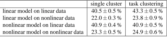
Table 1: Explained variance for each of the combinations of model and database. single cluster task clustering linear model on linear data 40.5±0.5 % 43.3±0.5 % linear model on nonlinear data 22.0±0.3 % 23.8±0.9 % nonlinear model on linear data 40.9±0.4 % 40.9±0.5 % nonlinear model on nonlinear data 23.3±0.5 % 24.9±0.6 %
with additional covariates. All covariates and responses were scaled per task (outlet) to zero mean and unit variance. Performance measures were obtained as for the school data, where now the ‘training set’ contains 100 samples per task and the ‘test set’ contains the remaining 56 samples. For the task-dependent mean and the gating of tasks we constructed two features depending on the outlet’s location: the first feature codes the number of local inhabitants (from zero, less than 15,000, to four, more than 300,000), the second one the level of tourism (from zero, hardly any tourism, to two, very touristic).
5.2 Generalization Performance
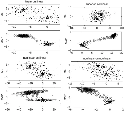
Artificial Data. We applied both the linear and the nonlinear method to the two databases we created, resulting in four combinations. In each of these four combinations we applied both the multitask learning method with one cluster, and model clustering. As can be seen in Figure 3, in all four cases the method was able to discern the two clusters. Note that in the second panel (linear model working on nonlinear data) one of the priors is ‘flattened’, indicating that in this case only part of the (nonlinear) structure could be found.
Table 1 presents a model evaluation in terms of the percentage of variance explained by both models with and without clustering. Percentage explained variance is defined as the total variance of the data minus the sum-squared error on the test set as a percentage of the total data variance. All combinations of model and database except the nonlinear model on the linear database showed significant improvements when task clustering is implemented. Note also that nonlinear multitask learning on the linear database performed equally well as the linear method. Apart from this, the nonlinear model worked best for the nonlinear database and the linear model for the linear database. For both databases, single task learning explained less than one percent of the variance.
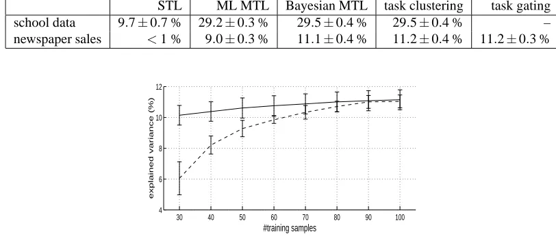
School Data. We applied single task learning, non-Bayesian and Bayesian multitask learning on the school data. The results are expressed in Table 2. Single task learning explained 9.7% of the variance, which was much less than any of the multitask learning methods. Non-Bayesian multitask learning explained 29.2% of the variance. The overall winners were the Bayesian methods with one and two priors (clusters) with an explained variance of 29.5%. Implementation of the methods described in Section 4 yielded no improvement on the ‘single cluster’ multitask learning method. This lack of improvement was also reflected in the clusters obtained: either two very similar priors were created, or one cluster was found to contain all tasks, whereas the other was empty. Although task clustering did not yield a significant improvement here, at least the results show that the method does not force structure on the data where there is no structure present.
Prediction of Newspaper Sales. The model of Section 2 (single Gaussian prior) managed to explain 11.1% of the variance in the test data, much better than the 9.0% explained variance with the same multitask model regularized through early stopping instead of through a ‘learned’ prior. Note that this regression problem has a very low signal-to-noise ratio, also due to the fact that, for a fair real-world comparison, only sales figures from at least four weeks ago can be used as covariates. When all tasks were optimized independently using all 13 covariates, less than one percent explained variance was achieved. These results are consistent with the more extended simulation studies in (Heskes, 1998, 2000).
−10 −5 0 −5
0 5
ML
linear on linear
−10 −5 0
−5 0 5
MAP
−100 −50 0 50 100
−10 0 10
ML
linear on nonlinear
−5 0 5 10 15 20
−5 0 5
MAP
−60 −40 −20 0 20
−5 0 5
ML
nonlinear on linear
−60 −40 −20 0 20
−5 0 5
MAP
−15 −10 −5 0 5
−5 0 5
nonlinear on nonlinear
ML
−6 −4 −2 0 2
−5 0 5
MAP
Figure 3: Maximum likelihood (upper panels, markedML) and maximum a posteriori (lower panels, marked
MAP) values for the model parameters Ai in the artificial data paradigm. Each dot or diamond refers to one task, where (in the lower panels) identical marks (dots or diamonds) indicate tasks that belong to the same cluster (are generated around the same mean). In each panel, the horizontal axis corresponds to the hidden-to-output weight, the vertical axis to the bias. The 95% confidence intervals for the two estimated priors are plotted in the lower panels. From left to right and up to down, the panels show the results for the linear model on the linear data, the same model on the nonlinear data, the nonlinear model on the linear data and on the nonlinear data. The means mα
used for generation of the data sets (corrected for the difference between the true and estimated hidden unit activity) are depicted by stars in the 8 panels.
Table 2: Explained variance for the school data and the newspaper data. The evaluated methods are sin-gle task learning (STL), maximum likelihood multitask learning (ML MTL), Bayesian multitask learning, task clustering with two clusters and task gating with two clusters.
STL ML MTL Bayesian MTL task clustering task gating school data 9.7±0.7 % 29.2±0.3 % 29.5±0.4 % 29.5±0.4 % – newspaper sales <1 % 9.0±0.3 % 11.1±0.4 % 11.2±0.4 % 11.2±0.3 %
30 40 50 60 70 80 90 100
4 6 8 10 12
explained variance (%)
#training samples
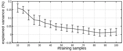
Figure 4: Explained variance for multitask learning with one (dashed line) and two clusters (solid line): for less training samples the effect of clustering grows stronger.
caused by the fact that for single task learning the input-to-hidden weights need to be optimized for each task separately, whereas these weights are equal for all tasks in the other methods.
More in general, multitask learning is most useful in circumstances where many parallel tasks are avail-able, but few training samples per task. To test under such conditions, we compared the single Gaussian prior model to the model with two clusters for lower numbers of training samples per task, ranging from 30 to 100 samples. Figure 4 shows the explained variances for both models, which are (as before) the averages over 10 independent splits of the data into a training and a test set. The figure clearly shows that although for larger numbers of training samples the more involved model does not perform much better than the simpler model, for less training samples it yields a substantial improvement.
5.3 Interpretation of the Newspaper Results
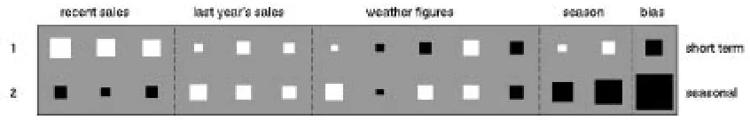
The solutions that we obtained make sense and provide a lot of interesting information. Figure 5 displays a Hinton diagram (Bishop, 1995) of the input-to-hidden weights typically and consistently (up to permutation and sign flips) found in all of the multitask learning approaches. It can be seen that one hidden unit focuses on recent sales figures (referred to as ‘short term’) and the other on last year’s sales and season (referred to as ‘seasonal’).
The left panel in Figure 6 plots the maximum likelihood solutions for the hidden-to-output weights of the different outlets. The next panel visualizes the effect of a single Gaussian prior by plotting the corresponding
MAP solutions. Task clustering yielded two distinct clusters: a ‘seasonal’ cluster with hardly any variation in short-term effects and a ‘short-term’ cluster with much less variation in the seasonal effect. The solution obtained through task gating is just slightly different. Although this particular distinction between the two clusters is not what we had expected to find (i.e. clusters with different means Mα and similar covariances
Figure 5: Hinton diagram of the input-to-hidden weights. Positive weights are white, negative weights are black. The absolute magnitude of each weight corresponds to the size of its square. Past sales figures are coded in the first 6 inputs, the next 5 inputs represent weather information, and the last 2 inputs indicate the season. The rightmost squares represent the biases of the hidden units.
−1 0 1 2
0
1
2
short term effects
maximum likelihood
−1 0 1 2
0
1
2
no clustering (MAP)
<−− seasonal effects −−>
−1 0 1 2
0
1
2
task clustering (MAP)
−1 0 1 2
0
1
2
task gating (MAP)
Figure 6: The maximum likelihood values for the hidden-to-output weights (left panel), and theirMAPvalues (right panels). The horizontal axis of each plot refers to the hidden-to-output weight connected to the hidden unit with input-to-hidden weights that are sensitive to seasonal effects, as demonstrated in Figure 5. The vertical axis refers to the weights connected to the hidden unit that is sensitive to short term effects. Each mark represents the hidden-to-output weights for one task. The ellipses drawn in the right panels visualize the priors imposed on the task-dependent parameters Ai. They indicate 95% confidence intervals of these priors. The prior depicted in the second panel is uni-modal (single cluster): all task-dependent weights have the same prior distribution. In the right two panels there are two clusters, formed through task clustering (third panel) and task gating (fourth panel).
the hidden unit that focuses on short term effects, yet they do display moderate to strong connections to the seasonal hidden unit. The reverse is true for the short term cluster.
Figure 7: Clustering of Dutch outlets. Circles mark outlets assigned with weight larger than 0.85 to either the ‘seasonal’ cluster (left panel) or the ‘short term’ cluster (right panel).
5.4 Difference Between Task Clustering and Task Gating
It is no surprise that task gating manages to pick up the correlations between short term or seasonal effects and location of the outlet. For example, after training the prior assignment of an outlet in a large non-touristic city to the short-term cluster equals 0.87, whereas an outlet in a small touristic village is assigned to the seasonal cluster with weight 0.80. The reason that this prior information does not lead to (significantly) better generalization performance is that the a posteriori assignments based on 100 training examples appear to be of about the same quality for task clustering and gating. With less examples, the a priori assignments will become more important (see Section 5.4), making the gating method preferable over the clustering approach, as can be seen in Figure 8.
Another way to illustrate the difference between task clustering and task gating is through the ‘entropy’ of the clusters formed by each method. We define the entropy of a set of clusters in this setting as
S(ρ) =−
N
∑
i=1
ncluster
∑
α=1
ρiαlog(ρiα),
where
ρiα=P(ziα=1|Λ,Di),
the probability for task i to be in clusterα. The entropy S(ρ)reaches its maximum when each task is assigned to any cluster with equal probability, and its minimum when each task is assigned to one particular cluster with probability one.
For both task clustering and gating the entropy depends on the number of samples present in the data D. For very low numbers of samples the cluster assignmentρiαwill depend mainly on the chosen prior, whereas for larger numbers of samples the data likelihood will become the dominant factor. Figure 9 plots the entropy for task assignments obtained from both methods as a function of the number of samples per task. The data set used here is the Telegraaf data set, but for the purpose of this illustration it could be any data set in which a meaningful clustering can be found.
10 20 30 40 50 60 70 80 90 100 −0.05
0 0.05 0.1 0.15 0.2
#training samples
exp
la
ine
d
var
iance
(%)
Figure 8: Difference in explained variance between the task gating and clustering approach: the less training samples, the better the gating method.
6. Related Work
Multitask learning is very similar to multilevel analysis in statistics. Here, a distinction is made between level one variation between different samples within the same task (e.g. from student to student, from patient to patient) and level two variation between different tasks (e.g. between schools or hospitals). The leading model to account for such variations is the mixed-effects linear model. In this model the user is presented with a series of parallel units, each containing a set of covariates and responses. The predicted value for the
µthresponse of unit i in this model reads
yµi =xµiTβ+zµiTbi,
where xµi is a vector of covariates,βis a vector of fixed effects parameters, biis the task-dependent random effect assumed to be (normal) distributed around zero with covarianceΣand zµi is a vector of parameters re-lated to this effect. The parameters in this model are generally estimated through iteration of linear regression on the parametersβ, and fitting of the covarianceΣto the residuals ˜yµi =yµi −xµiTβ. An alternative to this method is the empirical Bayesian approach, where probability distributions over both bi andβare defined. The parameters of these distributions (called hyperparameters) are optimized directly, resulting in distribu-tions around the maximum a posteriori values for biandβ. Both approaches are described in e.g. (Bryk and Raudenbush, 1992). In the full Bayesian approach (see e.g. Seltzer et al., 1996) further prior distributions are defined for these hyperparameters, which are chosen a priori. In this approach, however, one has to resort to sampling, which becomes infeasible for large numbers of tasks.
Over the past years many proposals have been made to incorporate nonlinearity into these models, through B-splines (see e.g. Lin and Zhang, 1999) and other methods (Brumback and Rice, 1998, Arora et al., 1997). To the best of our knowledge, the ideas of task clustering and gating are new to this field.
An alternative approach to multitask learning has been taken by Thrun and O’Sullivan (1996) and Pratt (1992), who have devised elegant ways to transfer knowledge obtained by one network to another network learning a similar task. Thrun and O’Sullivan (1996) also suggest a task clustering algorithm, where a distance metric between parallel tasks is learned, and used to classify new learning tasks. In learning these new tasks, (only) the information contained in the corresponding cluster is exploited.
Trajectory clustering (Cadez et al., 2000) can be derived as a special case of task clustering without hidden units and with all covariance matricesΣαset to zero. On a more philosophical level, clustering in our approach is an interesting by-product of a better generalizing model, not a goal by itself.
0 10 20 30 40 50 60 70 80 90 100 140
150 160 170 180 190 200 210 220 230 240
entropy
#training samples
Figure 9: The entropy of the task-cluster assignment probabilitiesρiαas a function of the number of samples for the task clustering method (dashed line) and the gating method (solid line). For few samples, the gating method clusters more strongly (has a lower entropy) than the task clustering method. For higher numbers of samples, the two methods behave similarly.
7. Discussion
Our work has been inspired by Baxter (1997), Caruana (1997) and Thrun and O’Sullivan (1996). We have adopted the idea of recognizing parallel tasks and learning their underlying structure from the data, and considered an extension through the use of task clustering, which has been implemented in a different form by Thrun and O’Sullivan (1996). In the present article we implement this clustering through the design of prior distributions that are able to discriminate between tasks. The result is a hierarchical Bayesian approach to multitask learning, where some of the model parameters are shared explicitly (the input-to-hidden weights among others) and others are soft-shared through a prior distribution. Two of these prior distributions make use of task-dependent features which are known in advance, the other distribution makes the distinction between tasks purely from the data samples in the training set. The applicability of this model to real-world problems was demonstrated (among others) on the newspaper data, where we showed the usefulness of the model both in terms of explained variance and independent detection of features in the data.
Application of our methods on an artificial data set demonstrated that appropriately structured regression problems can benefit significantly both from the multitask learning approach and from task clustering. The well-known school problem was also modeled better through Bayesian multitask learning. No substructures within the collection of tasks were found however, either because they are not present at all, or because another form of (neural network) model (e.g. other transfer functions than tanh(x) or linear) is needed to exploit them. For the Telegraaf problem we found a small yet significant increase in explained variance when task clustering was applied. However, simulations for smaller numbers of training samples showed a much more substantial improvement for smaller data sets. Interesting results were obtained on a descriptive level: the model was able to make a meaningful distinction between outlets in touristic and urban areas, without being presented with this information in advance. By examining the obtained clusters more closely, a better understanding of the tasks themselves can be gained.
We have assumed from the start that all of the parallel tasks may be assumed iid given the hyperparame-ters. Although for the artificial data this is true by construction, for the newspaper data it may not be entirely correct. In fact, each task in this database describes a time series, and parallel tasks imply parallel times. In this paper we have made no use of any algorithm specifically designed to model such data. In future work however, we plan to further extend our model to exploit this characteristic of the data. Here we hope to make a connection between multilevel analysis and dynamic hierarchical models (Gamerman and Migon, 1993). Acknowledgements
This research was supported by the Technology FoundationSTW, applied science division ofNWOand the technology programme of the Ministry of Economic Affairs.
We would like to thank Prof. Snijders and Prof. Eisinga for their support and advice.
Appendix A
The data likelihood is calculated as follows:
P(Di|Λ) =
Z
dAiP(Di,Ai|Λ)
= Z dAiP(Di|Ai,Λ)P(Ai|Λ)
∝ σ−ni|Σ|−1/2 Z
dAiexp
−1 2A
T
iQiAi+RTi Ai− 1 2Si
∝ σ−ni|Σ|−1/2|Qi|−21exp
1 2(R
T
iQ−i 1Ri−Si)
,
where Qi, Riand Siare given by
Qi = σ−2 ni
∑
µ=1
hµihµiT+Σ−1, Ri=σ−2 ni
∑
µ=1
yµihµi+Σ−1m, Si=σ−2 ni
∑
µ=1
yµi2+mTΣ−1m.
For the linear case, the expressions for Qi, Riand Sisimplify considerably by enforcing the constraint
hihTi
=W xixTiW
=I
(whereh..idenotes the average over all examples µ and I is the unit matrix):
Qi = niσ−2I+Σ−1, Ri=σ−2niWhxiyii+Σ−1m, Si=σ−2ni
y2i+mTΣ−1m.
In this case, sufficient statistics can be calculated beforehand, after which optimizing the shared parameters no longer scales with the number of tasks (Heskes, 2000).
Appendix B
To optimize log P(D|Λ), first we add the parameter z, which refers to a particular choice of cluster assignments
obtain
log P(Di|Λ) = log
∑
{z}
P(Di,z|Λ)
= log
∑
{z}
P(z|Λn,Di)
P(Di,z|Λ)
P(z|Λn,Di)
≥
∑
{z}
P(z|Λn,Di)log P(Di,z|Λ)−
∑
{z}
P(z|Λn,Di)log P(z|Λn,Di)
=
∑
{z}
P(z|Λn,Di)log P(Di|z,Λ) +
∑
{z}
P(z|Λn,Di)log P(z|Λ),
where we dropped the negative term in the third line since it does not depend onΛ. In the E-step we have to compute the assignments probabilities through
P(ziα=1|Λ,Di)∝qαP(Di|Λ).
and sum log P(Di|z,Λ)and log P(z|Λ)over all possible assignments, weighted by their probabilities. Note that if the assignments were not given, the log-likelihood of D would read
log P(D|Λ) =
∑
i log
∑
αqαP(Di|Λα),
which due to the summation within the log function would be much more difficult to maximize.
After each maximization (M-step) we set Λn=Λ, and take a next step, until convergence. With this choice ofΛn(standard for the EM-algorithm) the Jensen bound in line 3 becomes an equality, and the bound ensures that in the subsequent maximization step log P(D|Λ)will never decrease.
Appendix C
Table 3 presents the parameters that are used to generate the artificial data in Section 5.1. Note that W andσ do not vary between clusters.
Table 3: Numerical values for the parameters generating the linear and nonlinear data.
linear data cluster 1 cluster 2
W 0.023 −1.24 −0.041 0.023 −1.24 −0.041
mα −3.67 3.63 0.048 −2.43
Σα
0.80 0.23 0.23 1.19
0.97 −0.23 −0.23 1.07
σ 5 5
nonlinear data cluster 1 cluster 2
W 0.033 −0.62 −0.051 0.033 −0.62 −0.051
mα −3.67 3.63 0.048 −2.43
Σα
0.80 0.23 0.23 1.19
0.97 −0.23 −0.23 1.07
W0 0.27 0.27
References
M. Aitkin and N. Longford. Statistical modelling issues in school effectiveness studies. Journal of the Royal
Statistical Society A, 149:1–43, 1986.
V. Arora, P. Lahiri, and K. Mukherjee. Empirical Bayes estimation of finite population means from complex surveys. Journal of the American Statistical Association, 92:1555–1562, 1997.
J. Baxter. A Bayesian/information theoretic model of learning to learn via multiple task sampling. Machine
Learning, 28:7–39, 1997.
C. Bishop. Neural Networks for Pattern Recognition. Oxford: Clarendon Press, 1995.
B. Brumback and J. Rice. Smoothing spline models for the analysis of nested and crossed samples of curves.
Journal of the American Statistical Association, 93:961–976, 1998.
S. Bryk and W. Raudenbush. Hierarchical linear models: applications and data analysis methods. Sage Publications, Inc, Newbury Park (CAL), 1992.
I. Cadez, S. Gaffney, and P. Smyth. A general probabilistic framework for clustering individuals and objects. In Proceedings of the ACM SIGKDD Conference, pages 140–149, 2000.
R. Caruana. Multitask learning. Machine Learning, 28:41–75, 1997.
R. Caruana, S. Lawrence, and C. Lee Giles. Overfitting in neural networks: Backpropagation, conjugate gradient, and early stopping. In Advances in Neural Information Processing Systems 13, pages 402–408, Denver, Colorado, 2001. MIT Press.
M. Daniels and C. Gatsonis. Hierarchical generalized linear models in the analysis of variations in health care utilization. Journal of the American Statistical Association, 94:29–38, 1999.
A. Dempster, N. Laird, and D. Rubin. Maximum likelihood from incomplete data via the EM algorithm.
Journal of the Royal Statistical Society B, 39:1–38, 1977.
D. Gamerman and H. Migon. Dynamic hierarchical models. Journal of the Royal Statistical Society, Ser. B, 55:629–642, 1993.
T. Heskes. Solving a huge number of similar tasks: a combination of multi-task learning and hierarchical Bayesian modeling. In ICML, pages 233–241, 1998.
T. Heskes. Empirical Bayes for learning to learn. In P. Langley, editor, Proceedings of ICML, pages 367–374, San Francisco, CA, 2000. Morgan Kaufmann.
W. Jiang and M. Tanner. On the approximation rate of hierarchical mixtures-of-experts for generalized linear models. Neural Computation, 11:1183–1198, 1999.
M. Jordan and R. Jacobs. Hierarchical mixtures of experts and the EM algorithm. Neural Computation, 6: 181–214, 1994.
X. Lin and D. Zhang. Inference in generalized additive mixed models by using smoothing splines. Journal
of the Royal Statistical Society, 61:381–400, 1999.
D. MacKay. Probable networks and plausible predictions – a review of practical Bayesian methods for supervised neural networks. Network, 6:469–505, 1995.
P. Mortimore, P. Sammons, L. Stoll, D. Lewis, and R. Ecob. School Matters. Wells: Open Books, 1988. L. Pratt. Discriminability-based transfer between neural networks. In Advances in Neural Information
C. Robert. The Bayesian Choice: A Decision-Theoretic Motivation. Springer, New York, 1994.
M. Seltzer, H. Wong, and A. Bryk. Bayesian analysis in applications of hierarchical models: issues and methods. Journal of Educational and Behavioral Statistics, 21:131–167, 1996.
S. Thrun and J. O’Sullivan. Discovering structure in multiple learning tasks: The TC algorithm. In
Interna-tional Conference on Machine Learning, pages 489–497, 1996.
C. Williams and D. Barber. Bayesian classification with Gaussian processes. IEEE Transactions on Pattern