Machine Learning Methods for Predicting Failures
in Hard Drives: A Multiple-Instance Application
Joseph F. Murray [email protected]
Electrical and Computer Engineering, Jacobs Schools of Engineering University of California, San Diego
La Jolla, CA 92093-0407 USA
Gordon F. Hughes [email protected]
Center for Magnetic Recording Research University of California, San Diego La Jolla, CA 92093 USA
Kenneth Kreutz-Delgado [email protected]
Electrical and Computer Engineering, Jacobs Schools of Engineering University of California, San Diego
La Jolla, CA 92093-0407 USA
Editor: Dale Schuurmans
Abstract
We compare machine learning methods applied to a difficult real-world problem: predicting com-puter hard-drive failure using attributes monitored internally by individual drives. The problem is one of detecting rare events in a time series of noisy and nonparametrically-distributed data. We develop a new algorithm based on the multiple-instance learning framework and the naive Bayesian classifier (mi-NB) which is specifically designed for the low false-alarm case, and is shown to have promising performance. Other methods compared are support vector machines (SVMs), unsuper-vised clustering, and non-parametric statistical tests (rank-sum and reverse arrangements). The failure-prediction performance of the SVM, rank-sum and mi-NB algorithm is considerably bet-ter than the threshold method currently implemented in drives, while maintaining low false alarm rates. Our results suggest that nonparametric statistical tests should be considered for learning problems involving detecting rare events in time series data. An appendix details the calculation of rank-sum significance probabilities in the case of discrete, tied observations, and we give new recommendations about when the exact calculation should be used instead of the commonly-used normal approximation. These normal approximations may be particularly inaccurate for rare event problems like hard drive failures.
Keywords: hard drive failure prediction, rank-sum test, support vector machines (SVM), exact nonparametric statistics, multiple instance naive-Bayes
1. Introduction
Hard drive manufacturers have been developing self-monitoring technology in their products since 1994, in an effort to predict failures early enough to allow users to backup their data (Hughes et al., 2002). This Self-Monitoring and Reporting Technology (SMART) system uses attributes collected during normal operation (and during off-line tests) to set a failure prediction flag. The SMART flag is a one-bit signal that can be read by operating systems and third-party software to warn users of impending drive failure. Some of the attributes used to make the failure prediction include counts of track-seek retries, read errors, write faults, reallocated sectors, head fly height too low or high, and high temperature. Most internally-monitored attributes are error count data, implying positive integer data values, and a pattern of increasing attribute values (or their rates of change) over time is indicative of impending failure. Each manufacturer develops and uses its own set of attributes and algorithm for failure prediction. Every time a failure warning is triggered the drive can be returned to the factory for warranty replacement, so manufacturers are very concerned with reducing the false alarm rates of their algorithms. Currently, all manufacturers use a threshold algorithm which triggers a SMART flag when any single attribute exceeds a predefined value. These thresholds are set conservatively to avoid false alarms at the expense of predictive accuracy, with an acceptable false alarm rate on the order of 0.1% per year (that is, one drive in 1000). For the SMART algorithm currently implemented in drives, manufacturers estimate the failure detection rate to be 3-10%. Our previous work has shown that by using nonparametric statistical tests, the accuracy of correctly detected failures can be improved to as much as 40-60% while maintaining acceptably low false alarm rates (Hughes et al., 2002; Hamerly and Elkan, 2001).
In addition to providing a systematic comparison of prediction algorithms, there are two main novel algorithmic contributions of the present work. First, we cast the hard drive failure predic-tion problem as a multiple-instance (MI) learning problem (Dietterich et al., 1997) and develop a new algorithm termed multiple-instance naive Bayes (mi-NB). The mi-NB algorithm adheres to the strict MI assumption (Xu, 2003) and is specifically designed with the low false-alarm case in mind. Our second contribution is to highlight the effectiveness and computational efficiency of nonparametric statistical tests in failure prediction problems, even when compared with powerful modern learning methods. We show that the rank-sum test provides good performance in terms of achieving a high failure detection rate with low false alarms at a low computational cost. While the rank-sum test is not a fully general learning method, it may prove useful in other problems that involve finding outliers from a known class. Other methods compared are support vector machines (SVMs), unsupervised clustering using the Autoclass software of Cheeseman and Stutz (1995) and the reverse-arrangements test (another nonparametric statistical test) (Mann, 1945). The best per-formance overall was achieved with SVMs, although computational times were much longer and there were many more parameters to set.
The methods described here can be used in other applications where it is necessary to detect rare events in time series including medical diagnosis of rare diseases (Bridge and Sawilowsky, 1999; Rothman and Greenland, 2000), financial forecasting such as predicting business failures and personal bankruptcies (Theodossiou, 1993), and predicting mechanical and electronic device failure (Preusser and Hadley, 1991; Weiss and Hirsh, 1998).
1.1 Previous Work in Hard Drive Failure Prediction
used was from the Quantum Corporation, and contained data from two drive models. The data set used in the present paper is from a different manufacturer, and includes many more attributes (61 vs. 14), which is indicative of the improvements in SMART monitoring that have occurred since the original paper. An important observations made by Hughes et al. (2002) was that many of the SMART attributes are nonparametrically distributed, that is, their distributions cannot be easily characterized by standard parametric statistical model (such as normal, Weibull, chi-squared, etc.). This observation led us to investigate nonparametric statistical tests for comparing the distribution of a test drive attribute to the known distribution of good drives. Hughes et al. (2002) compared single-variate and multivariate rank-sum tests with simple thresholds. The single-variate test was combined for multiple attributes using a logical OR operation, that is, if any of the single attribute tests indicated that the drive was not from the good population, then the drive was labeled failed. The OR-ed test performed slightly better than the multivariate for most of the region of interest (low false alarms). In the present paper we use only the single-variate rank-sum test (OR-ed decisions) and compare additional machine learning methods, Autoclass and support vector machines. An-other method for SMART failure prediction, called naive Bayes EM (expectation-maximization), using the original Quantum data was developed by Hamerly and Elkan (2001). The naive Bayes EM is closely related to the Autoclass unsupervised clustering method used in the present work. Using a small subset of the features provided better performance than using all the attributes. Some preliminary results with the current SMART data were presented in Murray et al. (2003).
1.2 Organization
This paper is organized as follows: In Section 2, we describe the SMART data set used here, how it differs from previous SMART data and the notation used for drives, patterns, samples, etc. In Sec-tion 3, we discuss feature selecSec-tion using statistical tests such as reverse arrangements and z-scores. In Section 4, we describe the multiple instance framework, our new algorithm multiple-instance naive-Bayes (mi-NB), the failure prediction algorithms, including support vector machines, unsu-pervised clustering and the rank-sum test. Section 5 presents the experimental results comparing the classifiers used for failure prediction and the methods of preprocessing. A discussion of our results is given in Section 6 and conclusions are presented in Section 7. An Appendix describes the calculation of rank-sum significance levels for the discrete case in the presence of tied values, and new recommendations are given as to when the exact test should be used instead of the standard approximate calculation.
2. Data Description
The data set consists of time series of SMART attributes from a single drive model, and is a different data set than that used in Hughes et al. (2002); Hamerly and Elkan (2001).1 Data from 369 drives were collected, and each drive was labeled good or failed, with 178 drives in the good class and 191 drives in the failed class. Drives labeled as good were from a reliability test, run in a controlled environment by the manufacturer. Drives labeled as failed were returned to the manufacturer from users after a failure. It should be noted that since the good drive data were collected in a controlled uniform environment and the failed data come from drives that were operated by users, it is rea-sonable to expect that there will be differences between the two populations due to the different
Pattern
of n = 5
samples
N total
samples
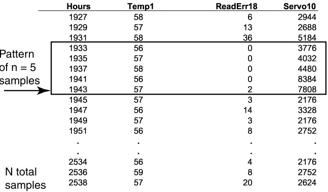
Figure 1: Selected attributes from a single good drive. Each row of the table represents a sample (all attributes recorded for a single time interval). The box shows the n selected consecutive samples in each pattern xjused to make a failure prediction at the time pointed at by the
arrow. The first sample available in the data set for this drive is from Hours = 1927, as only the most recent 300 samples are stored in drives of this model.
manner of operation. Algorithms that attempt to learn the difference between the good and failed populations may in fact be learning this difference and not the desired difference between good and nearly-failing drive samples. We highlight this point to emphasize the importance of understanding the populations in the data and considering alternative reasons for differences between classes.
A sample is all the attributes for a single drive for a single time interval. Each SMART sam-ple was taken at two hour intervals in the operating drives, and the most recent 300 samsam-ples are saved on the disk. The number of available valid samples for each drive i is denoted Ni, and Ni
may be less than 300 for those drives that did not survive 600 hours of operation. Each sample contains the drive’s serial number, the total power-on-hours, and 60 other performance-monitoring attributes. Not all attributes are monitored in every drive, and the unmonitored attributes are set to a constant, non-informative value. Note that there is no fundamental reason why only 300 samples were collected; this was a design choice made by the drive manufacturer. Methods exist by which all samples over the course of the drive’s life can be recorded for future analysis. Figure 1 shows some selected attributes from a single good drive, and examples of samples (each row) and patterns (the boxed area). When making a failure prediction a pattern xj ∈Rn·a(where a is the number of
attributes) is composed of the n consecutive samples and used as input to a classifier. In our exper-iments n was a design parameter which varied between 1 and 100. The pair(Xi,
Y
i)represents thedata in each drive, where the set of patterns is Xi= [x1, . . . ,xNi]and the classification is
Y
i∈ {0,1}.For drives labeled good,
Y
i=0 and for failed drivesY
i=1.and possibly different methods of measurement. Also, all good and failed drive data were collected during a single reliability test (whereas in the current set, the failed drives were returns from the field).
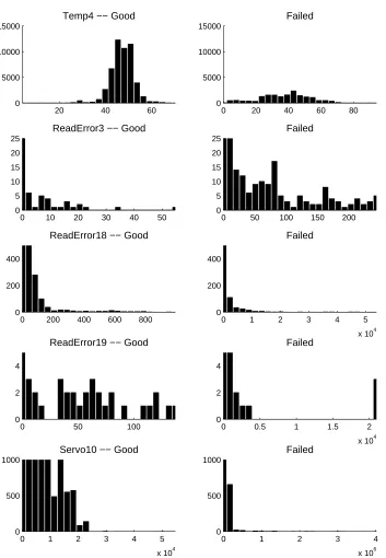
A preliminary examination of the current set of SMART data was done by plotting the his-tograms of attributes from good and failed drives. Figure 2 shows hishis-tograms of some representa-tive attributes. As was found with earlier SMART data, for many of the attributes the distributions are difficult to describe parametrically as they may be multimodal (such as the Temp4 attribute) or very heavy tailed. Also noteworthy, many attributes have large numbers of zero values, and these zero-count bins are truncated in the plots. These highly non-Gaussian distributions initially lead us to investigate nonparametric statistical tests as a method of failure prediction. For other pattern recognition methods, special attention should be paid to scaling and other preprocessing.
3. Feature Selection
The process of feature selection includes not only deciding which attributes to use in the classifier, but also the number of time samples, n, used to make each decision, and whether to perform a preprocessing transformation on these input time series. Of course, these choices depend strongly on which type of classifier is being used, and issues of feature selection will also be discussed in the following sections.
As will be demonstrated below, some attributes are not strongly correlated with future drive failure and including these attributes can have a negative impact on classifier performance. Because it is computationally expensive to try all combinations of attribute values, we use the fast nonpara-metric reverse-arrangements test and attribute z-scores to identify potentially useful attributes. If an attribute appeared promising with either method it was considered for use in the failure detection algorithms (see Section 4).
3.1 Reverse Arrangements Test
The reverse arrangements test is a nonparametric test for trend which is applied to each attribute in the data set (Mann, 1945; Bendat and Piersol, 2000). It is used here based on the idea that a pattern of increasing drive errors is indicative of failure. Suppose we have a time sequence of observations of a random variable, xi,i=1...N. In our case xi could be, for example, the seek error count of
the most recent sample. The test statistic, A=∑Ni=1−1Ai, is the sum of all reverse arrangements,
where a reverse arrangement is defined as an occurrence of xi>xjwhen i< j. To find A we use the
intermediate sums Aiand the indicator function hi j,
Ai= N
∑
j=i+1
hi j where hi j=I(xi>xj) .
We now give an example of calculating A for the case of N=10. With data x (which is assumed to be a permutation of the ranks of the measurements),
x= [x1, . . . ,x10] = [1,4,3,7,2,8,6,10,9,5], the values of Aifor i=1. . .9 are found,
A1=
10
∑
j=2
h1 j=0, A2= 10
∑
j=3
h2 j=2, . . . A9= 10
∑
j=9
20 40 60 0
5000 10000 15000
Temp4 −− Good
0 20 40 60 80 0
5000 10000 15000
Failed
0 10 20 30 40 50 0
5 10 15 20 25
ReadError3 −− Good
0 50 100 150 200 0
5 10 15 20 25
Failed
0 200 400 600 800 0
200 400
ReadError18 −− Good
0 1 2 3 4 5
x 104 0
200 400
Failed
0 50 100
0 2 4
ReadError19 −− Good
0 0.5 1 1.5 2
x 104 0
2 4
Failed
0 1 2 3 4 5
x 104 0
500 1000
Servo10 −− Good
0 1 2 3 4
x 106 0
500 1000
Failed
with the values[Ai] = [0,2,1,3,0,2,1,2,1]. The test statistic A is the sum of these values, A=12.
For large values of N, the test statistic A is normally distributed under the null hypothesis of no trend (all measurements are random with the same distribution) with mean and variance (Mann, 1945),
µA=
N(N−1)
4 , σ
2
A=
2N3+3N2−5N
72 .
For small values of N, the distribution can be calculated exactly by a recursion (Mann, 1945, eq. 1). First, we find the count CN(A)of permutations of{1,2, . . . ,N}with A reverse arrangements,
CN(A) = A
∑
i=A−N+1
CN−1(i),
where CN(A) =0 for A<0 and C0(A) =0. Since every permutation is equally likely with probability 1
n! under the null hypothesis, the probability of A is CN(A)
n! .
Tables of the exact significance levels of A have been made. For significance levelα, Appendix Table A.6 of Bendat and Piersol (2000) gives the acceptance regions,
AN;1−α/2<A≤AN;α/2,
for the null hypothesis of no trend in the sequence xi(that is, that xiare independent observations of
the same underlying random variable).
The test is formulated assuming that the measurements are drawn from a continuous distribution, so that the ranks x are distinct (no ties). SMART error count data values are discrete and allow the possibility of ties. It is conventional in rank-based methods to add random noise to break the ties, or to use the midrank method described in Section 4.6.
3.2 Z-scores
The z-score compares the mean values of each attribute in either class (good or failed). It is calcu-lated over all samples,
z=rmf−mg σ2
f nf +
σ2 g ng
,
where mf andσ2f are the mean and variance of the attribute in failed drives, mgandσ2gare the mean
and variance in good drives, nf and ng are the total number of samples of failed and good drives.
Large positive z-scores indicate the attribute is higher in the population of failed drive samples, and that there is likely a significant difference in the means between good and failed samples. However, it should be noted that the z-score was developed in the context of Gaussian statistics, and may be less applicable to nonparametric data (such as the error count attributes collected by hard drives).
3.3 Feature Selection for SMART Data
non-negative integers). The percentage of drives for which the null hypothesis of no trend is rejected is calculated for good and failed drives. Table 3.3 lists attributes and the percent of drives that have significant trends for the good and failed populations. The null hypothesis (no trend) was accepted for 1968≤A≤2981, for a significance level higher than 99%. We are interested in attributes that have both a high percentage of failed drives with significant trends and a low percentage of good drives with trends, in the belief that an attribute that increases over time in failed drives while remaining constant in good drives is likely to be informative in predicting impending failure.
From Table 3.3 we can see that attributes such as Servo2, ReadError18 and Servo10 could be useful predictors. Note that these results are reported for a test of one group of 100 samples from each drive using a predefined significance level, and no learning was used. This is in contrast to the way a failure prediction algorithm must work, which must test each of many (usually N) consecutive series of samples, and if any fail, then the drive is predicted to fail (see Section 4.1 for details).
Some attributes (for example CSS) are cumulative, meaning that they report the number of occurrences since the beginning of the drive’s life. All cumulative attributes either will have no trend (nothing happens) or have a positive trend. Spin-ups is the number of times the drive motors start the platters spinning, which happens every time the drive is turned on, or when it reawakens from a low-power state. It is expected that most drives will be turned on and off repeatedly, so it is unsurprising that both good and failed drives show increasing trends in Table 1. Most attributes (for example ReadError18) report the number of occurrences during the two-hour sample period.
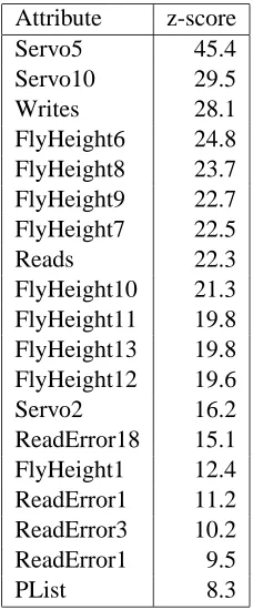
Table 3.3 lists selected attributes sorted by descending z-score. Attributes near the top are initially more interesting because of more significant differences in the means, that is, the mean value of an attribute (over all samples) for failed drives was higher than for good drives. Only a few of the attributes had negative z-scores, and of these even fewer were significant. Some attributes with negative z-scores also appeared to be measured improperly for some drives.
From the results of the reverse arrangements and z-score tests, a set of 25 attributes2was selected by hand from those attributes which appear to be promising due to increasing attribute trends in failed drives and large z-score values. The tests also help eliminate attributes that are not measured correctly, such as those with zero or very high variance.3 This set of attributes was used in the SVM, mi-NB and clustering algorithms (see the next section). Individual attributes in this set were tried one at a time with the rank-sum test. Attributes that provided good failure detection with low false alarms in the classifiers were then used together (see Section 5).
We note that the feature selection process is not a black-box automatic method, and required trial-and-error testing of attributes and combinations of attributes in the classifiers. Many of the attributes that appeared promising from the z-score and reverse-arrangements tests did not actually work well for failure prediction, while other attributes (such as ReadError19) were known to be im-portant from our previous work and from engineering and physics knowledge of the problem gained from discussions with the manufacturers. While an automatic feature selection method would be ideal, it would likely involve a combinatorial optimization problem which would be computationally expensive.
2. Attributes in the set of 25 are: GList1, PList, Servo1, Servo2, Servo3, Servo5, ReadError1, ReadError2, ReadError3, FlyHeight5, FlyHeight6, FlyHeight7, FlyHeight8, FlyHeight9, FlyHeight10, FlyHeight11, FlyHeight12, ReadEr-ror18, ReadError19, Servo7, Servo8, ReadError20, GList2, GList3, Servo10.
Attribute % Good % Failed Temp1 11.8% 48.2% Temp3 34.8% 42.9%
Temp4 8.4% 58.9%
GList1 0.6% 10.7%
PList 0.6% 3.6%
Servo1 0.0% 0.0%
Servo2 0.6% 30.4%
Servo3 0.6% 0.0%
CSS 97.2% 92.9%
ReadError1 0.0% 0.0% ReadError1 0.6% 5.4% ReadError3 0.0% 0.0% WriteError 1.1% 0.0% ReadError18 0.0% 41.1% ReadError19 0.0% 0.0%
Servo7 0.6% 0.0%
ReadError20 0.0% 0.0%
GList3 0.0% 8.9%
Servo10 1.7% 39.3%
Table 1: Percent of drives with significant trends by the reverse arrangements test for selected at-tributes, which indicates potentially useful attributes. Note that this test is performed only on the last n=100 samples of each drive, while a true failure prediction algorithm must test each pattern of n samples taken throughout the drives’ history. Therefore, these results typically represent an upper bound on the performance of a reverse-arrangements classi-fier. CSS are cumulative and are reported over the life of the drive, so it is unsurprising that most good and failed drives show increasing trends (which simply indicate that the drive has been turned on and off).
set would likely lead to high-variance error estimates (the variance of which cannot be estimated). We note that for all the classification error results in Section 5, the test set was not seen during the training process. The issue just discussed relates to the question of whether we have biased the re-sults by having performed statistical tests on the complete data set and used those rere-sults to inform our (mostly manual) feature and attribute selection process. The best solution is to collect more data from drives to validate the false alarm and detection rates, which a drive manufacturer would do in any case to test the method and set the operating curve level before actual implementation of improved SMART algorithms in drives.
Attribute z-score Servo5 45.4 Servo10 29.5 Writes 28.1 FlyHeight6 24.8 FlyHeight8 23.7 FlyHeight9 22.7 FlyHeight7 22.5
Reads 22.3
FlyHeight10 21.3 FlyHeight11 19.8 FlyHeight13 19.8 FlyHeight12 19.6 Servo2 16.2 ReadError18 15.1 FlyHeight1 12.4 ReadError1 11.2 ReadError3 10.2 ReadError1 9.5
PList 8.3
Table 2: Attributes with large positive z-score values.
4. Failure Detection Algorithms
We describe how the pattern recognition algorithms and statistical tests are applied to the SMART data set for failure prediction. First, we discuss the preprocessing that is done before the data is presented to some of the pattern recognition algorithms (SVM and Autoclass); the rank-sum and reverse-arrangements test require no preprocessing. Next, we develop a new algorithm called multiple-instance naive-Bayes (mi-NB) based on the multiple-instance framework and especially suited to low-false alarm detection. We then describe how the SVM and unsupervised clustering (Autoclass) algorithms are applied. Finally we discuss the nonparametric statistical tests, rank-sum and reverse-arrangements.
drive is used (see Figure 1). The length of x is(n×a) where a is the number of attributes. There are N vectors x created, with zeros prepended to those x in the early history of the drive. Results are not significantly different if the early samples are omitted (that is, N−n vectors are created) and this method allows us to make SMART predictions in the very early history of the drive. If any x is classified as failed, then the drive is predicted to fail. Since the classifier is applied repeatedly to all N vectors from the same drive, each test must be very resistant to false alarms.
4.1 Preprocessing: Scaling and Binning
Because of the nonparametric nature of the SMART data, two types of preprocessing were consid-ered: binning and scaling. Performance comparison of the preprocessing is given in Section 5.
The first type of preprocessing is binning (or discretization), which takes one of two forms: equal-frequency or equal-width (Dougherty et al., 1995). In equal-frequency binning, an attributes’ values are converted into discrete levels such that the number of counts at each level is the same (the discrete levels are percentile groups). In equal-width binning, each attribute’s range is divided into a fixed number of equal magnitude bins and values are converted into bin numbers. In both cases, the levels are set based on the training set. In both the equal-width and equal-frequency cases, the rank-order with respect to bin is preserved (as opposed to converting the attribute into multiple binary nominal attributes, one for each bin). Because there are a large number of zeros for some attributes in the SMART data (see Figure 2), a special zero-count bin is used with both equal-width and equal-frequency binning. The two types of binning were compared using the Autoclass and SVM classifiers. For the SVM, the default attribute scaling in the algorithm implementation (MySVM) was also compared to binning (see 4.4).
Binning (as a form of discretization) is a common type of preprocessing in machine learning and can provide certain advantages in performance, generalization and computational efficiency (Frank and Witten, 1999; Dougherty et al., 1995; Catlett, 1991). As shown by Dougherty et al. (1995), discretization can provide performance improvements for certain classifiers (such as naive Bayes), and that while more complex discretization methods (such as those involving entropy) did provide improvement over binning, the difference in performance between binning and the other methods was much smaller than that between discretization and no discretization. Also, binning can reduce overfitting resulting in a simpler classifier which may generalize better (Frank and Witten, 1999). Preserving the rank-order of the bins so that the classifier may take into account the ordering information (which we do) has been shown to be an improvement over binning into independent nominal bins (Frank and Witten, 1999). Finally, for many algorithms, it is more computationally efficient to train using binned or discretized attributes rather than numerical values. Equal-width binning into five bins (including the zero-count bin) was used successfully by Hamerly and Elkan (2001) on the earlier SMART data set, and no significant difference was found using up to 20 bins.
4.2 The Multiple-Instance Framework
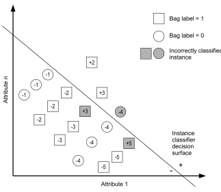
of the instances is labeled 1, then the bag label is 1. This method of classifying a bag as 1 if any of its instances is labeled 1 is known as the MI assumption. Because the instance labels are unknown, the goal is to learn the labels, knowing that at least one of the instances in each 1 bag has label 1, and all the instance labels in each 0 bag should be 0.
The hard drive problem can be fit naturally into the MI framework. Each pattern x (composed of n samples) is an instance, and the set of all patterns for a drive i is the bag Xi. The terms bag
label and drive label are interchangeable, with failed drives labeled
Y
i=1 and good drives labeledY
i =0. The hidden instance (pattern) labels are yj,j=1. . .Ni for the Ni instances in each bag(drive). Figure 3 show a schematic of the MI problem.
The multiple-instance framework was originally proposed by Dietterich et al. (1997) and applied to a drug activity prediction problem; that of discovering which molecules (each of which may exist in a number of different shapes, the group of all shapes for a specific molecule comprising a bag) bind to certain receptors, specifically that of smell receptors for the scent of musk. The instances consist of 166 attributes that represent the shape of one possible configuration of a molecule from X-ray crystallography, and the class of each molecule (bag) is 1 if the molecule (any instance) smells like musk as determined by experts. The so-called “musk” data sets have become the standard benchmark for multiple-instance learning.
The algorithm developed by Dietterich et al. (1997) is called axis-parallel-rectangles, and other algorithms were subsequently developed based on many of the paradigms in machine learning such as support vector machines (Andrews et al., 2003), neural networks, expectation-maximization, nearest-neighbor (Wang and Zucker, 2000), as well as special purpose algorithms like the diverse-density algorithm. An extended discussion of many of these is given by Xu (2003), who makes the important distinction between two classes of MI algorithms: those which adhere to the MI assumption (as described above) and those which make other assumptions, most commonly that the label for each positive bag is determined by some other method than simply if one instance has a positive label. Algorithms that violate the MI assumption usually assume that the data from all instances in a bag is available to make a decision about the class. Such algorithms are difficult to apply to the hard drive problem, as we are interested in construction on-line classifiers that make a decision based on each instance (pattern) as it arrives. Algorithms that violate the MI-assumption include Citation-k-Nearest-Neighbors (Wang and Zucker, 2000), SVMs with polynomial minimax kernel, and the statistical and wrapper methods of Xu (2003), and these will not be considered further for hard drive failure prediction.
4.3 Multiple Instance Naive Bayes (mi-NB)
We now develop a new multiple instance learning algorithm using naive Bayes (also known as the simple Bayesian classifier) and specifically designed to allow control of the false alarm rate. We call this algorithm mi-NB (multiple instance-naive Bayes) because of its relation to the mi-SVM algorithm of Andrews et al. (2003). The mi-SVM algorithm does adhere to the MI assumption and so could be used for the hard drive task, but since it requires repeated relearning of an SVM, it is presently too computationally intensive. By using the fast naive Bayes algorithm as the base classifier, we can create an efficient multiple-instance learning algorithm.
The mi-NB algorithm begins by assigning a label yjto each pattern: for good drives, all patterns
are assigned yj =0; for failed drives, all patterns except for the last one in the time series are
Figure 3: Multiple-instance learning. The numbers are bag (drive) numbers, and each circle or square represents an instance (pattern). Instances from class +1 (failed drives) are squares, while instances from class 0 are circles. The + or - in each instance represents the hidden underlying class of each instance, 1 or 0 respectively. The decision surface represents the classification boundary induced by a classifier. Grayed instances are those misclassified by the decision surface. Bag 1: All - instances are classified correctly, and the bag is correctly classified as 0 (good drive). Bag 2: One instance is classified as +, so the bag is correctly classified as 1 (failed drive). Bag 3: One instance of the failed drive is classified as -, but another is classified as +, so the bag is correctly classified (failed). Bag 4: An instance with true class - is labeled +, so the bag is misclassified as 1 (false alarm). Bag 5: All instances of the + bag (failed drive) are classified as -, so the bag is misclassified as 0 (missed detection).
naive Bayes model is trained (see below). Using the NB model, each pattern in the training set is assigned to a classybj∈ {0,1}. Because nearly all patterns are assigned to the good class yj=0, this
initial condition insures that the algorithm will start with a low false alarm rate. In each iteration of the mi-NB algorithm, for every failed drive
Y
i=1 that was misclassified (that is, all patterns wereclassified as good,ybj =0), the pattern j∗(with current label yj=0) that is most likely to be from
the failed class, j∗= arg max
j∈{1...Ni|yj=0}
set increases to over the target level, FA>FAtarget. The mi-NB algorithm is detailed in Algorithm 1. The procedure given in Algorithm 1 may be applied with different base classifiers other than naive Bayes, although the resulting algorithm may be computationally expensive unless there is an efficient way to update the model without retraining from scratch. Other stopping conditions could also be used, such as detection rate greater than a certain value or number of iterations.
Algorithm 1 mi-NB Train (for SMART failure prediction) Input: x,
Y
, FAdesired(desired false alarm rate)Initialize:
Good drives: For drives with
Y
i=0 initialize yj=0 for j=1. . .NiFailed drives: For drives with
Y
i=1 initialize yj=0 for j=1. . .Ni−1, and yNi =1Learn NB model
b
yj=arg max
c∈{0,1}fc(xj) Classify each pattern using the NB model Find FA and DET rate
while FA<FAtarget do
for all Misclassified failed drives,byj=0∀ j=1. . .Ni do
j∗= arg max
j∈{1...Ni|yj=0}
f1(xj) Find pattern closest to decision surface with label yj=0
yj∗←1 Reclassify the pattern as failed Update NB model
end for
b
yj=arg max
c∈{0,1}fc(xj) Reclassify each pattern using the NB model Find FA and DET rate
end while
Return: NB model
In Bayesian pattern recognition, the maximum a posterior (MAP) method is used to estimate the classby of a pattern x,
b
y=arg max
c∈{0,1}p(y=c|x) =arg max
c∈{0,1}p(x|y=c)p(y=c).
The “naive” assumption in naive Bayes is that the class-conditional distribution p(x|y=c)is fac-torial (independent components), p(x|y=c) =∏n·a
m=1p(xm|y=c) where n·a is the size of x (see
Section 2). The class estimate becomes,
fc(x) = n·a
∑
m=1
logpb(xm|y=c) +logpb(y=c)
b
y=arg max
c∈{0,1}fc(x), (1)
where we have used estimates bp of the probabilities. Naive Bayes has been found to work well in practice even in cases where the components xm are not independent, and a discussion of this
number elements #{·}can be found. Training a naive Bayes classifier is then a matter of finding the smoothed empirical estimates,
b
p(xm=k|y=c) =
#{xm=k,y=c}+`
#{y=c}+2`
b
p(y=c) = #{y=c}+`
#{patterns}+2`, (2) where ` is a smoothing parameter, which we set to `=1 corresponding to Laplace smoothing (Orlitsky et al. (2003), who also discuss more recent methods for estimating probabilities, including those based on the Good-Turing estimator). Ng and Jordan (2002) show that naive Bayes has a higher asymptotic error rate (as the amount of training data increases) but that it approaches this rate more quickly than other classifiers and so may be preferred in small-sample problems. Since each time we have to switch a pattern in the mi-NB iteration, we only have to change a few of the counts in (2), updating the model after relabeling certain patterns is very fast.
Next, we show that the mi-NB algorithm has non-decreasing detection and false alarm rates over the iterations.
Lemma 1 At each iteration t, the mi-NB algorithm does not decrease the detection and false alarm
rates (as measured on the training set) over the previous iteration t−1,
f1(t−1)(xj)≤ f( t) 1 (xj)
f0(t−1)(xj)≥ f0(t)(xj) ∀j=1. . .N. (3) Proof At iteration t−1 the probability estimates for a certain k are,
b
pt−1(xm=k|y=1) =
b+` d+2`,
where b=#{xm=k,y=c},d =#{y=c}, and of course b≤d. Since class estimates are always
switched from yj=0 to 1, for some k
b
pt(xm=k|y=1) =
b+`+1 d+2`+1
(and for other k it will remain constant). It is now shown that the conditional probability estimates are non-decreasing,
b
pt−1(xm=k|y=1) ≤ bpt(xm=k|y=1) (b+`)(d+2`+1) ≤ (d+2`)(b+`+1)
b ≤ d+` ,
with equality only in the case of b=d, `=0. Similarly, the prior estimate is also non-decreasing,
b
pt−1(y=1)≤bpt(y=1). From (1) this implies that f1(t−1)(x)≤ f1(t)(x).
For class y=0, it can similarly be shown that pbt−1(xm=k|y=0)≥ pbt(xm=k|y=0) and
b
Note that Algorithm 1 never relabels a failed pattern as a good pattern, as this might reduce the detection rate (and invalidate the proof of Lemma 1 in Section 4.3). The initial conditions of the algorithm ensure a low false alarm rate, and the algorithm proceeds (in a greedy fashion) to pick patterns that are mostly likely representatives of the failed class without re-evaluating previous choices. A more sophisticated algorithm could be designed that moves patterns back to the good class as they become less likely failed candidates, but this requires a computationally expensive combinatorial search.
4.4 Support Vector Machines (SVMs)
The support vector machine (SVM) is a popular modern pattern recognition and regression algo-rithm. First developed by Vapnik (1995), the principle of the SVM classifier is to project the data into a higher dimensional space where the classes are separated by a linear hyperplane which is defined by a small set of support vectors. For an introduction to SVMs for pattern recognition, see Burges (1998). The hyperplane is found by a quadratic optimization problem, which can be for-mulated for either the case where the patterns are linearly separable, or the non-linearly separable case which requires the use of slack variablesξifor each pattern and a parameter C that penalizes
the slack. We use the non-linearly separable case and in addition use different penalties L+,L−for incorrectly labeling each class. The hyperplane is found by solving,
min
w,b,ξ 1 2kwk
2+C
∑
∀i|yi=+1
L+ξi+
∑
∀i|yi=−1
L−ξi
!
subject to: yi(wTφ(xi) +b)≥1−ξi ξi≥0
where w and b are the parameters of the hyperplane by=wTφ(x) +b and φ(·) is the mapping to the high-dimensional space implicit in the kernel k(xj,xk) =φ(xj)Tφ(xk) (Burges, 1998). In the
hard-drive failure problem, L+penalizes false alarms, and L−penalizes missed detections. Since C is multiplied by both L+and L−, there are only two independent parameters and we set L−=1 and adjust C,L+when doing a grid search for parameters.
To apply the SVM to the SMART data set, drives are randomly assigned into training and test sets for a single trial. For validation, means and standard deviations of detection and false alarm rates are found over 10 trials, each with different training and test sets. Each pattern is assigned to the same label as the drive (all patterns in a failed drive
Y
=1 are assigned to the failed class, yi = +1, and all patterns in good drivesY
=0 are set to yi =−1). Multiple instance learningalgorithms like mi-SVM (Andrews et al., 2003) could be used to find a better way of assigning pattern classes, but these add substantial extra computation to the already expensive SVM training. We use the MySVM4package developed by Ruping (2000). Parameters for the MySVM soft-ware are set as follows: epsilon=10−2, max iterations=10000, convergence epsilon=10−3. When equal-width or equal-frequency binning is used (see Section 4.1), no scale is set; otherwise, the default attribute scaling in MySVM is used. The parameters C and L+ (with L−=1) are var-ied to adjust the tradeoff between detection and false alarms. Kernels tested include dot product, polynomials of degree 2 and 3, and radial kernels with width parameterγ.
4.5 Clustering (Autoclass)
Unsupervised clustering algorithms can be used for anomaly detection. Here, we use the Autoclass package (Cheeseman and Stutz, 1995) to learn a probabilistic model of the training data from only good drives. If any pattern is an anomaly (outlier) from the learned statistical model of good drives, then that drive is predicted to fail. The expectation maximization (EM) algorithm is used to find the highest-likelihood mixture model that fits the data. A number of forms of the probability den-sity function (pdf) are available, including Gaussian, Poisson (for integer count data) and nominal (unordered discrete, either independent or covariant). For the hard drive problem, they are all set to independent nominal to avoid assuming a parametric form for any attribute’s distribution. This choice results in an algorithm very closely related to the naive Bayes EM algorithm (Hamerly and Elkan, 2001), which was found to perform well on earlier SMART data.
Before being presented to Autoclass the attribute values are discretized into either equal-freq-uency bins or equal-width bins (Section 4.1), where the bin range is determined by the maximum range of the attribute in the training set (of only good drives). An additional bin was used for zero-valued attributes. The training procedure attempts to find the most likely mixture model to account for the good drive data. The number of clusters can also be determined by Autoclass, but here we have restricted it to a small fixed number from 2 to 10. Hamerly and Elkan (2001) found that for the naive Bayes EM algorithm, 2 clusters with 5 bins (as above) worked best. During testing, the estimated probability of each pattern under the mixture model is calculated. A failure prediction warning is triggered for a drive if the probability of any of its samples is below a threshold (which is a parameter of the algorithm). To increase robustness, the input pattern contained between 1 and 15 consecutive samples n of each attribute (as described above for the SVM). The Autoclass threshold parameter was varied to adjust tradeoff between detection and false alarm rates.
4.6 Rank-sum Test
The Wilcoxon-Mann-Whitney rank-sum test is used to determine if the two random data sets arise from the same probability distribution (Lehmann and D’Abrera, 1998, pg. 5). One set T comes from the drive under test and the other R is a reference set composed of samples from good drives. The use of this test requires some assumptions to be made about the distributions underlying the attribute values and the process of failure. Each attribute has a good distribution G and an about-to-fail distribution F. For most of the life of the drive, each attribute value is chosen from the G, and then at some time before failure, the values begin to be chosen from F. This model posits an abrupt change from G to F, however, the test should still be expected to work if the distribution changes gradually over time, and only give a warning when it has changed significantly from the reference set.
The test statistic WSis calculated by ranking the elements of R (of size m) and T (of size n) such
that each element of R and T has a rank S∈[1,n+m]with the smallest element assigned S=1. The rank-sum WSis the sum of the ranks S of the test set.
If the set sizes are large enough (usually, if the smaller set n>10 or m+n>20), the rank-sum statistic WSis normally distributed under the null hypothesis (T and R are from the same population)
due to the central limit theorem, with mean and variance:
E(WS) = 1
2n(m+n+1) Var(WS) =
mn(m+n+1)
12 −CT,
where CT is the ties correction, defined as
CT=
mn
e ∑ i=1
(di3−di)
12(m+n)(m+n−1),
where e is the number of distinct values in R and T , and di is the number of tied elements at each
value (see Appendix A for more details). The probability of a particular WScan be found using the
standard normal distribution, and a critical valueαcan be set at which to reject the null hypothesis. In cases of smaller sets where the central limit theorem does not apply (or where there are many tied values), an exact method of calculating the probability of the test statistic is used (see Appendix A, which also gives examples of calculating the test statistic).
For application to the SMART data, the reference set R for each attribute (size m=50 for most experiments) is chosen at random from the samples of good drives. The test set T (size n=15 for most experiments) is chosen from consecutive samples of the drive under test. If the test set for any attribute over the history of the drive is found to be significantly different from the reference set R then the drive is predicted to fail. The significance levelα is adjusted in the range[10−7,10−1]
to vary the tradeoff between false alarms and correct detections. We use the one-sided test of T coming from a larger distribution than R, against the hypothesis of identical distributions.
Multivariate nonparametric rank-based tests that exploit correlations between attribute values have been developed (Hettmansperger, 1984; Dietz and Killeen, 1981; Brunner et al., 2002). A different multivariate rank-sum test was successfully applied to early SMART data (Hughes et al., 2002). It exploits the fact that error counts are always positive. Here, we use a simple OR test to use two or more attributes: if the univariate rank-sum test for any attribute indicates a different distribution from the reference set, then that pattern is labeled failed. The use of the OR test is motivated by the fact that very different significance level ranges (per-pattern) for each attribute were needed to achieve low false alarm rates (per-drive).
4.7 Reverse Arrangements Tests
5. Results
In this section we present results from a representative set of experiments conducted with the SMART data. Due to the large number of possible combinations of attributes and classifier pa-rameters, we could not exhaustively search this space, but we hope to have provided some insight into the hard drive failure prediction problem and a general picture of which algorithms and prepro-cessing methods are most promising. We also can clearly see that some methods are significantly better than the current industry-used SMART thresholds implemented in hard drives (which provide only an estimated 3-10% detection rate with 0.1% false alarms).
5.1 Failure Prediction Using 25 Attributes
Figure 4 shows the failure prediction results in the form of a Receiver Operating Characteristic (ROC) curve using the SVM, mi-NB, and Autoclass classifiers with the 25 attributes selected be-cause of promising reverse arrangements test or z-score values (see Section 3.3). One sample per pattern was used, and all patterns in the history of each test drive were tested. (Using more than one sample per pattern with 25 attributes proved too computationally expensive for the SVM and Autoclass implementations, and did not significantly improve the mi-NB results.) The detection and false alarm rates were measured per drive: if any pattern in the drive’s history was classified as failed, the drive was classified as failed. The curves were created by performing a grid search over the parameters of the algorithms to adjust the trade-off between false alarms and detection. For the SVM, the radial kernel was used with the parameters adjusted as follows: kernel widthγ∈
[0.01,0.1,1], capacity C∈[0.001,0.01,0.1,1], the cost penalty L+∈[1,10,100]. Table 5.3 shows the parameters used in all SVM experiments. For Autoclass, the threshold parameter was adjusted in[99.99,99.90,99.5,99.0,98.5]and the number of clusters was adjusted in[2,3,5,10].
Although all three classifiers appear to have learned some aspects of the problem, the SVM is superior in the low false-alarm region, with 50.6% detection and no measured false alarms. For all the classifiers, it was difficult to find parameters that yielded low enough false alarm rates compared with the low 0.3-1.0% annual failure rate of hard drives. For mi-NB, even at the initial condition (which includes only the last sample from each failed drive in the failed class) there is a relatively high false alarm rate of 1.0% at 34.5% detection.
For the 25 attributes selected, the SVM with the radial kernel and default scaling provided the best results. Results using the linear kernel with the binning and scaling are shown in Figure 5. The best results with the linear kernel were achieved with the default scaling, although it was not possible to adjust to false alarm rate to 0%. Equal-width binning results in better performance than equal-frequency binning for SVM and Autoclass. The superiority of equal-width binning is consistent with other experiments (not shown) and so only equal-width binning will be considered in the remaining sections. Using more bins (10 vs. 5) for the discretization did not improve performance, confirming the results of Hamerly and Elkan (2001).
0 5 10 15 0
10 20 30 40 50 60 70 80
False alarms (%)
Detection (%)
SVM, radial mi−NB
Autoclass, EW bins Autoclass, EF bins
Figure 4: Failure prediction performance of SVM, mi-NB and Autoclass using 25 attributes (one sample per pattern) measured per drive. For mi-NB, the results shown are for equal-width binning. Autoclass is tested using both equal-equal-width (EW) and equal-frequency (EF) binning (results with 5 bins shown). Error bars are±1 standard error in this and all subsequent figures.
0 5 10 15
0 10 20 30 40 50 60 70 80
False alarms (%)
Detection (%)
SVM, default scaling SVM, EW bins SVM, EF bins
Also of interest is how far in advance we are able to predict an imminent failure. Figure 7 shows a histogram of the time before actual failure that the drives are correctly predicted as failing, plotted for SVM at the point 50.6% detection, 0.0% false alarms. The majority of detected failures are predicted within 100 hours (about 4 days) before failure, which is a long enough period to be reasonable for most users to backup their data. A substantial number of failures were detected over 100 hours before failure, which is one of the motivations for initially labeling all patterns from failed drives as being examples of the failed class (remembering that our data only includes the last 600 hours of SMART samples from each drive).
5.2 Single-attribute Experiments
In an effort to understand which attributes are most useful in predicting imminent hard-drive failure, we tested the attributes individually using the non-parametric statistical methods (rank-sum and re-verse arrangements). The results of the rere-verse arrangements test on individual attributes (Section 3 and Table 3.3) indicate that attributes such as ReadError18 and Servo2 could have high sensitiv-ity. The ReadError18 attribute appears promising with 41.1% of failed drives and 0 good drives showing significant increasing trends. Figure 8 shows the failure prediction results using only the ReadError18 attribute with the rank-sum, reverse arrangements, and SVM classifiers. Reducing the number of attributes from 25 to 1 increases the speed of all classifiers, and this increase is enough so that more samples can be used per pattern, with 5 samples per pattern used in Figure 8. The rank-sum test provided the best performance, with 24.3% detection with false alarms too low to measure, and 33.2% detection with 0.5% false alarms. The mi-NB and Autoclass algorithms using the ReadError18 (not shown in Figure 8 for clarity) perform better than the reverse-arrangements test and slightly worse than the SVM.
Single attribute tests using rank-sum were run on all 25 attributes selected in Section 3.3 with 15 samples per pattern. Of these 25, only 8 attributes (Figure 9) were able to detect failures at suf-ficiently low false alarm rates: ReadError1, ReadError2, ReadError3, ReadError18, ReadError19, Servo7, GList3 and Servo10. Confirming the observations of the feature selection process, ReadEr-ror18 was the best attribute, with 27.6% detection at 0.06% false alarms.
For the rank-sum test, the number of samples to use in the reference set (samples from good drives) is an adjustable parameter. Figure 10 shows the effects of using reference set sizes 25, 50 and 100 samples, with no significant improvement for 100 samples over 50. For all other rank-sum test results 50 samples were used in the reference set.
5.3 Combinations of Attributes
Using combinations of attributes in the rank-sum test can lead to improved results over single-attribute classifiers (Figure 11). The best single single-attributes from Figure 9 were ReadError1, Read-Error3, ReadError18 and ReadError19. Using these four attributes and 15 samples per pattern, the rank-sum test detected 28.1% of the failures, with no measured false alarms. Higher detection rates (52.8%) can be had if more false alarms are allowed (0.7%). These four attributes were also tested with the SVM classifier (using default scaling). Interestingly, the linear kernel provided better performance than the radial, illustrating the need to evaluate different kernels for each data set.
0 100 200 300 400 500 600
Figure 4 (25 attributes)
SVM
mi−NB
Autoclass
Figure 11 (4 attributes)
SVM
Ranksum
Time (min)
Algorithm
Figure 6: Training times (in minutes) for each of the algorithms used in Figures 4 and 11. The train-ing times shown are averaged over a set of parameters. The total traintrain-ing time includes a search over multiple parameters. For example, the SVM used in Figure 4 required a grid search over 36 points which took a total of 17893 minutes for training with parameter se-lection. For the rank-sum test, only one parameter needs to be adjusted, and the training time for each parameter value was 2.2 minutes, and 21 minutes for the search through all parameters.
0 100 200 300 400 500 600
0 50 100 150 200
Hours before failure
# of drives
0 0.5 1 1.5 2 2.5 3 3.5 4 4.5 5 0
10 20 30 40 50
False alarms (%)
Detection (%)
Rank−sum SVM − radial Rev. Arr.
Figure 8: Failure prediction performance of classifiers using a single attribute, ReadError18, with 5 input samples per pattern. For rank-sum and reverse arrangements, error bars are smaller than line markers. For this attribute, the SVM performed best using the radial kernel and default attribute scaling (no binning).
rates of<1%, this means that some of the trials had no false alarm drives while other trials had very few (1 or 2). Because some drives are inherently more likely to be predicted as false alarms, whether these drives are included in the test or training sets can lead to a variance from trial to trial, causing large error bars at some of the points.
6. Discussion
We discuss the results of our findings and their implications for hard-drive failure prediction and machine learning in general.
0 1 2 3 0 10 20 30 40 50 ReadError1 Detection (%) Ranksum
0 1 2 3
0 10 20 30 40 50 ReadError2
0 1 2 3
0 10 20 30 40 50 ReadError3 Detection (%)
0 1 2 3
0 10 20 30 40 50 ReadError18
0 1 2 3
0 10 20 30 40 50 ReadError19 Detection (%)
0 1 2 3
0 10 20 30 40 50 Servo7
0 1 2 3
0 10 20 30 40 50 GList3
False alarms (%)
Detection (%)
0 1 2 3
0 10 20 30 40 50 Servo10
False alarms (%)
Figure 9: Failure prediction performance of rank-sum using the best single attributes. The number of samples per pattern is 15, with 50 samples used in the reference set.
0 0.5 1 1.5 2 2.5 3 0
10 20 30 40 50
False alarms (%)
Detection (%)
Ranksum ref 25 Ranksum ref 50 Ranksum ref 100
Figure 10: Rank-sum test with reference set sizes 25, 50 and 100 using ReadError18 attribute and 15 test samples. There is no improvement in performance using 100 samples in the reference set instead of 50 (as in all other rank-sum experiments).
0 0.5 1 1.5 2 2.5 3
0 10 20 30 40 50 60
False alarms (%)
Detection (%)
Rank−sum SVM linear SVM radial
Figure 11: Failure prediction performance of rank-sum and SVM classifiers using four attributes: ReadError1, ReadError3, ReadError18 and ReadError19.
Figure 4
Point Detection False Alarm Kernel gamma C L+
L-1 50.60 0.00 radial 0.100 0.010 100.0 1.0
2 64.18 4.21 radial 0.010 0.100 100.0 1.0
3 70.38 6.20 radial 0.010 1.000 100.0 1.0
Figure 5
Point Detection False Alarm Kernel C L+
L-1 default scaling 54.73 0.78 linear 0.001 1000.0 1.0
2 60.97 3.09 linear 0.100 5.0 1.0
3 63.17 7.75 linear 0.010 5.0 1.0
1 EW bins 11.18 0.00 linear 0.001 100.0 1.0
2 41.40 0.46 linear 0.001 5.0 1.0
3 48.05 1.72 linear 0.001 1.0 1.0
4 51.83 8.68 linear 0.001 0.5 1.0
1 EF bins 17.54 2.34 linear 0.001 5.0 1.0
2 42.90 11.09 linear 0.100 5.0 1.0
3 (off graph) 70.22 35.40 linear 0.100 10.0 1.0
Figure 8
Point Detection False Alarm Kernel gamma C L+
L-1 8.28 0.00 radial 0.010 0.010 100.0 1.0
2 17.01 0.96 radial 0.100 0.010 1.0 1.0
3 30.29 3.45 radial 1.000 0.010 1.0 1.0
Figure 11
Point Detection False Alarm Kernel gamma C L+
L-1 linear 5.43 0.17 linear 0.001 1000.0 1.0
2 15.82 0.35 linear 0.010 1000.0 1.0
3 32.92 0.51 linear 0.010 1.0 1.0
4 52.23 0.96 linear 0.100 1.0 1.0
1 radial 1.68 0.09 radial 0.100 0.001 100.0 1.0
2 9.29 0.53 radial 0.001 0.010 100.0 1.0
3 17.79 0.69 radial 1.000 1.000 1000.0 1.0
4 27.13 1.73 radial 0.100 0.100 100.0 1.0
Table 3: Parameters for SVM experiments in Figures 4, 5, 8 and 11.
imminent failure. Also of interest, although with less selectivity, are attributes that measure seek errors.
labels of those good samples mostly likely to be from the failed distribution. This semi-supervised approach can be contrasted with the unsupervised Autoclass and the fully supervised SVM, where all patterns from failed drives were labeled failed.
The reverse-arrangements test performed more poorly than expected, as we believed that the assumption of increasing trend made by this test was well suited for hard drive attributes (like read-error counts) that would presumably increase before a failure. The rank-sum test makes no as-sumptions about trends in the sets, and in fact all time-order information is removed in the ranking process. The success of the rank-sum method led us to speculate that this removal of time-order over the sample interval was important for failure prediction. There are physical reasons in drive tech-nology why impending failure need not be associated with an increasing trend in error counts. The simplest example is sudden stress from a failing drive component which causes a sudden increase in errors, followed by drive failure.
It was also found that a small number of samples (from 1 to 15) in the input patterns was suf-ficient to predict failure accurately, this indicates that the drive’s performance can degrade quickly, and only a small window of samples is needed to make an accurate prediction. Conversely, using too many samples may dilute the weight of an important event that occurs within a short time frame. One of the difficulties in conducting this research was the need to try many combinations of attributes and classifier parameters in order to construct ROC curves. ROC curves are necessary to compare algorithm performance because the cost of misclassifying one class (in this case, false alarms) is much higher than for the other classes. In many other real world applications such as the examples cited in Section 1, there will also be varying costs for misclassifying different classes. Therefore, we believe it is important that the machine learning community develop standardized methods and software for the systematic comparison of learning algorithms that include cycling through ranges of parameters, combinations of attributes and number of samples to use (for time series problems). An exhaustive search may be prohibitive even with a few parameters, so we envi-sion an intelligent method that attempts to find the broad outline of the ROC curve by exploring the limits of the parameter space, and gradually refines the curve estimate as computational time allows. Another important reason to create ROC curves is that some algorithms (or parameterizations) may perform better in certain regions of the curve than others, with the best algorithm dependent on the actual costs involved (which part of the curve we wish to operate in).
7. Conclusions
We have shown that both nonparametric statistical tests and machine learning methods can signifi-cantly improve over the performance of the hard drive failure-prediction algorithms which are cur-rently implemented. The SVM achieved the best performance of 50.6% detection/0% false alarms, compared with the 3-10% detection/0.1-0.3% false alarms of the algorithms currently implemented in hard drives. However, the SVM is computationally expensive for this problem and has many free parameters, requiring a time-consuming and non-optimal grid search.
achieved with base classifiers other than naive Bayes, for example, the mi-SVM algorithm (An-drews et al., 2003) could be suitably adapted but probably remains computationally prohibitive.
We also showed that the nonparametric rank-sum test can be useful for pattern recognition and that it can have higher performance than SVMs for certain combinations of attributes. The best performance was achieved using a small set of attributes: the rank-sum test with four attributes predicted 28.1% of failures with no false alarms (and 52.8% detection/0.7% false alarms). Attributes useful for failure prediction were selected by using z-scores and the reverse arrangements test for increasing trend.
Improving the performance of hard drive failure prediction will have many practical benefits. In-creased accuracy of detection will benefit users by giving them an opportunity to backup their data. Very low false alarms (in the range of 0.1%) will reduce the number of returned good drives, thus lowering costs to manufacturers of implementing improved SMART algorithms. While we believe the algorithms presented here are of high enough quality (relative to the current commercially-used algorithms) to be implemented in drives, it is still important to test them on larger number of drives (on the order of thousands) to measure accuracy to the desired precision of 0.1%. We also note that each classifier has many free parameters and it is computationally prohibitive to exhaustively search the entire parameter space. We choose many parameters by non-exhaustive grid searches; finding more principled methods of exploring the parameter space is an important topic of future research.
We hope that the insights we have gained in employing the rank-sum test, multiple-instance framework and other learning methods to hard drive failure prediction will be of use in other prob-lems where rare events must be forecast from noisy, nonparametric time series, such as in the pre-diction of rare diseases, electronic and mechanical device failures, and bankruptcies and business failures (see references in Section 1).
Acknowledgments
This work is part of the UCSD Intelligent Disk Drive Project funded by the Information Storage Industry Center (a Sloan Foundation Center), and by the UCSD Center for Magnetic Recording Re-search (CMRR). J. F. Murray gratefully acknowledges support by the ARCS Foundation. We wish to thank the anonymous reviewers work for their detailed and insightful comments and suggestions, particularly regarding the use of the multiple instance framework. We also thank the corporate sponsors of the CMRR for providing the data sets used in our work.
Appendix A: Exact and Approximate Calculation of the Wilcoxon-Mann-Whitney Significance Probabilities
The Wilcoxon-Mann-Whitney test is a widely used statistical procedure for comparing two sets of single-variate data (Wilcoxon, 1945; Mann and Whitney, 1947). The test makes no assumptions about the parametric form of the distributions each set is drawn from and so belongs to the class of nonparametric or distribution-free tests. It tests the null hypothesis that the two distributions are equal against the alternative that one is stochastically larger than the other (Bickel and Doksum, 1977, pg. 345). For example, two populations identical except for a shift in mean is sufficient but not necessary for one to be stochastically larger than the other.
Following Klotz (1966), suppose we have two sets X = [x1,x2, . . . ,xn] , Y = [y1,y2, . . . ,ym],
X 74 59 63 64 n = 4
Y 65 55 58 67 53 71 m = 6
[X,Y]sorted 53 55 58 59 63 64 65 67 71 74
Ranks 1 2 3 4 5 6 7 8 9 10
X ranks 10 4 5 6 WX = 25
Y ranks 7 2 3 8 1 9 WY = 30
Table 4: Calculating the Wilcoxon statistic WX and WY without ties
is assigned a rank according to its place in the sorted list. The Wilcoxon statistic WX is calculated
by summing the ranks of each xi, hence the term rank-sum test. Table 7 gives a simple example of
how to calculate WX and WY. If the two distributions are discrete, some elements may be tied at the
same value. In most practical situations the distributions are either inherently discrete or effectively so due to the finite precision of a measuring instrument. The tied observations are given the rank of the average of the ranks that they would have taken, called the midrank. Table 7 gives an example of calculating the Wilcoxon statistic in the discrete case with ties. There are five elements with the value ‘0’ which are all assigned the average of their ranks:(1+2+3+4+5)/5=3.
To test the null hypothesis H0 that the distributions F and G are equal against the alternative Ha that F(x)≤G(x)∀x, F 6=G we must find the probability p0=P(WX >wx) that under H0 the
true value of the statistic is greater than the observed value, now called wx(Lehmann and D’Abrera,
1998, pg. 11). If we were interested in the alternative that F≤G or F≥G, a two-sided test would be needed. The generalization to the two-sided case is straightforward and will not be considered here, see Lehmann and D’Abrera (1998, pg. 23). Before computers were widely available, values of p0 (the significance probability) were found in tables if the set sizes were small (usually m and n<10) or calculated from a normal approximation if the set sizes were large. Because of the number of possible combinations of tied elements, the tables and normal approximation were created for the simplest case, namely continuous distributions (no tied elements).
X 0 0 0 1 3 n = 5
Y 0 0 1 2 2 3 4 m = 7
X ranks 3 3 3 6.5 10.5 WX = 26
Y ranks 3 3 6.5 8.5 8.5 10.5 12 WY = 52
z1 z2 z3 z4 z5
Discrete values: 0 1 2 3 4
t1 t2 t3 t4 t5
Ties configuration: 5 2 2 2 1