Evolution at shifting range margins

(1)

Elizabeth Claire Elliott

Submitted in accordance with the requirements for the degree of Doctor of Philosophy

The University of Leeds

School of Biology

(2)

(3)

The candidate confirms that the work submitted is her own, except where work which has formed part of jointly authored publications has been included. The contribution of the candidate and the other authors to this work has been explicitly indicated below. The candidate confirms that appropriate credit has been given within the thesis where reference has been made to the work of others.

Chapter 2 contains work from a jointly authored publication:

Elliott, E. C. and Cornell, S. J. Dispersal polymorphism and the speed of biological invasions. PLoS One, 7: e40496, 2012.

Author contributions are as follows: ECE and SJC jointly designed the model. ECE carried out simulations of the model, calculated the invasion speeds and wrote the initial drafts of the manuscript. SJC gave guidance on the calculations in particular how to calculate when each invasion speed occurs and edited the final version of the manuscript.

Chapter 3 also contains work from a jointly authored publication:

Elliott E. C. and Cornell S. J. Are anomalous invasion speeds robust to demographic stochasticity? PLoS One 8: e67871, 2013.

Author contributions are as follows: ECE and SJC jointly designed the model. ECE carried out simulations of the model, calculated the invasion speeds and wrote the initial drafts of the manuscript. SJC gave guidance on the methods used for analysis, wrote Appendix S2 and edited the final version of the manuscript.

In the remaining chapters SJC was involved in discussions of the work, and in particular in Chapters 4 and 5 helped design the models and gave guidance on how to carry out the data analysis.

This copy has been supplied on the understanding that it is copyright material and that no quotation from the thesis may be published without proper acknowledgement.

c

2013 The University of Leeds, Elizabeth Claire Elliott

The right of Elizabeth Claire Elliott to be identified as Author of this work has been asserted by her in the accordance with the Copyright, Designs and Patents Act 1998.

(4)

Abstract

The speed at which biological range expansions occur has important consequences for species experiencing climate change, and for invasions by exotic organisms. There is growing empirical and theoretical evidence that during range expansions there is selection for increased dispersal, and that this can result in faster rates of spread. However, few models consider whether increased dispersal comes at a cost.

In this thesis I investigated how two different trade-offs between dispersal and other traits affected the rates of range expansions. The first modelled a direct trade-off between dispersal and reproduction, and the second incorporated a trade-off so that adaptation to an environmental gradient came at a cost to dispersal.

The first trade-off was investigated by modelling a population that consisted of two dispersal phenotypes, one that has a higher population growth rate and one that has a higher dispersal rate. Using a simple deterministic model it was found that when there was a big trade-off between the morphs in terms of these traits, anomalous invasion speeds were observed whereby a population consisting of both phenotypes invades at a speed faster than either single phenotype. It was found that these anomalous invasion speeds were robust to demographic stochasticty. Adding a shifting climate to the model revealed that a trade-off between dispersal and establishment ability can help a species to keep up with climate change.

The second trade-off was investigated using a quantitative trait model, which revealed that a trade-off between dispersal and adaptation can result in the formation of range margins. Introducing a shifting environment allowed a species to expand its range at a speed determined by the steepness of the gradient and the size of the trade-off.

These models reveal that trade-offs can alter range shifting dynamics, the consequences of which for predicting rates of range expansions were discussed.

(5)

In loving memory of my grandfather Alan Charles Elliott

(6)

Acknowledgements

I would first like to thank my supervisor, Stephen Cornell, who has provided support and guidance throughout my PhD. Stephen helped in the design of the models in this thesis and has taught me many new mathematical and numerical techniques without which I would not have not have been able to complete this work. I would also like to thank him for providing encouragement when things did not seem to be going right, and for always reminding me that if something was confusing that it made it more interesting!

I would like to thank my project advisor Tim Benton and the post-docs in my group Sandro Azaele and Omar Al Hammal for giving helpful advice during my PhD. I would also like to thank Bill Kunin and members of his lab group for interesting discussions at the weekly lab meetings, which broadened my scientific knowledge and where I was always given useful feedback on my work. I would particularly like to thank Laura Harrison for always helping to put things into perspective, and Richard German for his many helpful hints of tricks in R that made my code more efficient.

My time as part of the Ecology department at Leeds University has been enjoyable and I would like to thank everyone for always being friendly, in particular other occupants of the Manton 8.17 postgraduate office who have helped to provide a productive working environment. I would especially like to thank Rowena Mitchell, Kirsty Robertson and Rebeca Velazquez Lopez for becoming friends that I know will always be there for me.

Finally I would like to thank my friends outside of University and my family for providing encouragement and support even when they often did not understand what I have been doing during my PhD! I would particularly like to thank my parents and brother for always having a word of encouragement and supporting me throughout this time. Last but not least I want say a huge thank you to my partner Sam who has helped me throughout this time, providing morale support and having to cope with all my stresses and triumphs as a result of the ups and downs of doing a PhD.

(7)

List of figures

1.1 Growth and spread of a population . . . 10

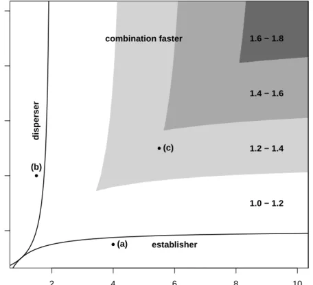
2.1 Parameter regions where each invasion speed occurs . . . 35

2.2 Invasion profile when there is no mutation between phenotypes . . . 36

2.3 Invasion profile when there is mutation between phenotypes . . . 38

2.4 Invasion profiles with different parameter values . . . 39

2.5 Comparison of analytical and numerical predictions of the invasion speed 43 3.1 Invasion profiles of the establisher and disperser morphs . . . 56

3.2 Comparison of analytical and numerical predictions of the invasion speed 59 3.3 Comparison of stochastic and deterministic invasion speeds at different carrying capacities . . . 60

3.4 Comparison of stochastic and deterministic invasion speeds for simulations carried out in 2D . . . 62

3.5 Comparison of invasion speeds with different values ofµ . . . 63

3.6 Comparison of invasion speeds with asymmetrical mutation rates between morphs . . . 64

3.7 Anomalous invasion speeds when individual morph speeds are similar . . 65

3.8 Comparison of population densities at the invasion front for the case where anomalous speeds occur . . . 67

3.9 Comparison of population densities at the invasion front where in (a) the invasion follows the speed of the establisher morph, and in (b) follows the speed of the disperser morph . . . 68

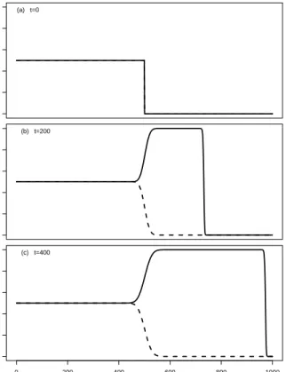
4.1 Range shifting of the population when the establisher is the faster morph . 78 4.2 Range shifting of the population when the disperser is the faster morph . . 79

4.3 Range shifting of the population when the individual morphs are slower than the rate of shifting . . . 80

(12)

4.4 Mean time to extinction of the population against log(carrying capacity) . 82

4.5 Mean time to extinction of the population against log(carrying capacity)

for a larger shifting landscape . . . 84

5.1 Form of dispersal function . . . 94

5.2 Travelling wave of invasion with no environmental gradient . . . 97

5.3 Invasion speed for different values ofz¯. . . 100

5.4 Formation of range margins for different values of the environmental gradient . . . 101

5.5 Formation of range margins with different initial conditions . . . 102

5.6 Range size scaled by the steepness of the environmental gradient . . . 103

5.7 Shape of the travelling wavefront when the gradient is shifting in time . . 106

5.8 Fluctuation in population density when the environmental gradient is shallow . . . 107

(13)

List of tables

1.1 Summary of theoretical studies investigating limits to species’ ranges . . 15

(14)

1. Introduction

1.1

Introduction: The importance of shifting range margins

Two of the most important threats to biodiversity are climate change and invasions by exotic species. During the past century, mean global surface temperatures have increased by 0.6◦C (IPCC, 2007). These temperatures are predicted to continue increasing, with a 1.8◦C best estimate of warming at the end of the 21st century under a low scenario, and a best estimate of 4◦C for the high scenario (IPCC, 2007). A changing climate may lead to what was formerly suitable habitat for a species becoming unsuitable. This poses a challenge for many species; species will need to either adapt to the new conditions, or shift with the conditions to which they are currently adapted.

1.1.1 Evidence of species shifting their ranges with climate change

There is lots of empirical evidence that species are shifting their ranges to higher latitudes and/or altitudes in response to recent warming (Chen et al., 2011; Hickling et al., 2006; Parmesan and Yohe, 2003; Root et al., 2003). It has been estimated using a meta-analysis that the distributions of species have shifted to higher latitudes at a median rate of 16.9 km per decade, and to higher elevations at a median rate of 11.0 m per decade (Chen et al., 2011). However, this response was found to vary greatly within taxonomic groups and between individuals (Chen et al., 2011; Moritz and Agudo, 2013), and has also been found to vary over time (Mair et al., 2012).

Not all species are able to respond to climate change by shifting their range, and even if they can they may not be able to track it at the same rate as the shifting climate. Evidence from British butterflies shows that many species are not keeping up with climate change (Menendez et al., 2006; Warren et al., 2001). Also, even if species are able to expand their range with climate change this does not necessarily mean that the species will increase in abundance. For example, in response to recent climate warming, the northern range margin of the small skipper butterfly, Thymelicus sylvestris, has shifted northwards, but this has been accompanied by a decrease in distribution area and abundance (Mair et al., 2012). There are numerous factors that affect whether a species is able to respond, many of which will interact with one another. Some of the main factors are discussed below.

(15)

Dispersal ability

Higher dispersal ability will mean a species is more likely to be able to track climate change, and so escape the adverse direct and indirect effects of increased temperatures (Watkinson and Gill, 2002) . For example, it has been found that faster northern range shifts are observed in more mobile butterflies living in forest edges in Finland (P¨oyry et al., 2009). In Britain, it has also been found that sedentary butterfly species tend to lag behind climate more than mobile species (Warren et al., 2001; Wilson et al., 2009). There is also growing evidence of evolutionary changes in dispersal in response to climate change (see Le Galliard et al., 2012, for a review), which will be discussed in more detail later in the Introduction.

Habitat fragmentation

Species may not be able to expand their ranges if they have to pass through areas of unsuitable habitat (Thomas et al., 2001), and this may result in species being unable to keep pace with climate change (Travis, 2003). For example, in Britain, the expansion rate of the silver-spotted skipper butterfly, Hesperia comma, is being controlled by habitat fragmentation (Wilson et al., 2009). There is also some evidence that species expanding their range have been found to disproportionately expand into protected areas, where habitat may be less fragmented (Thomas et al., 2012). This highlights the importance of having suitable habitat available for species to be able to expand into in response to climate change.

Species interactions

A single species may be limited or prevented from expanding its range as a result of interactions with other species (Berg et al., 2010). If interacting species have different dispersal rates the spatial association of two species may be interrupted (Callaway et al., 2004). For example, Kinlan and Gaines (2003) have shown that plants disperse over smaller distances than their herbivores; so although the herbivorous insects are able to track shifts in temperature, the plant hosts lag behind constraining the insects’ expansion.

However, novel species interactions may help species to expand their ranges. For example, the brown argus butterfly, Aricia agestis, has spread northwards in Britain 2.3 times faster than the average global expansion rate of species (Pateman et al., 2012). This

(16)

rapid expansion has occurred as a result of warmer conditions enabling this butterfly to use a new larval host plant in Britain (Pateman et al., 2012). This suggests that a change in interactions between species may in some cases facilitate range expansions.

1.1.2 Evidence of species responding to climate changein situ

Species that are unable to shift with the climate will need to respond to the new conditions in their current location in order to survive. Populations can do this either by adjusting to the new conditions by means of phenotypic plasticity, or by adapting to the new conditions by means of genetic changes through evolution (see Gienapp et al., 2008, for a review of the current evidence for each response). There is lots of evidence of plastic responses to climate change. For example, there is evidence that the timing of phenological events, such as bird nesting, first flowering and frog breeding has become earlier in response to increased temperatures (reviewed in Parmesan and Yohe, 2003). However, it is unlikely that species facing continued directional climate change will be able to survive by plastic responses alone in the long term (Gienapp et al., 2008).

There is limited evidence that some species have adapted by means of genetic changes to the conditions that have arisen as a result of climate warming. One of the few studies where genetic responses to increased temperatures have been observed is in the Canadian red squirrel, Tamiasciurus hudsonicus. In this squirrel, advanced parturition dates as a result of warmer springs have been shown to be a genetic response, resulting in earlier breeding (R´eale et al., 2003). Experimental evidence from yeast populations suggests that rapid evolution can help populations to survive environmental change (Bell and Gonzalez, 2009). However, further studies using genetic data are needed to be able to predict whether species will be able to survive climate change by adapting to new conditions.

1.1.3 Evidence of species extinctions as a result of climate change

If a species fails to adapt or to shift with the changing climate then it may become extinct. Predictions about future extinctions as a result of climate change vary, with one study estimating that between 18 and 35% of terrestrial species could become extinct by 2050, depending on the level of warming (Thomas et al., 2004). It is uncertain whether extinctions will ultimately reach this level, but there is evidence that species are becoming locally extinct at their lower latitude range margins. Range contractions have been observed in montane butterfly species as they have failed to adapt to increased

(17)

temperatures at their lower elevation range margins (Franco et al., 2006; Wilson et al., 2005).

There is also some evidence that species have already become extinct as a result of climate change. For example, 67% of harlequin frogs in the tropics have gone missing and presumed extinct in recent years as a result of increased night time temperatures spreading fungal pathogens (Pounds et al., 2006). Indeed, in a review of how climate change causes extinctions Cahill et al. (2012) found that changing species interactions as a result of climate change are an important cause of extinctions.

1.1.4 Evidence of invasions by exotic species

Native species are also being threatened by the invasion of their ranges by exotic species. Exotic species have been introduced accidentally or deliberately throughout the world, and when these species spread and become pests (Ziska et al., 2011), this has economic impacts and important consequences for biodiversity (Gurevitch and Padilla, 2004; Sakai et al., 2001). For example, the introduction of the cane toad,Bufo marinus, into Australia to control sugar cane pests was unsuccessful, and instead the cane toad has caused declines in native species (Urban et al., 2008).

Climate change will also have an impact on invasive species (Hellmann et al., 2008). One impact is that climate change is enabling exotic species to further expand their ranges into areas in which they would not historically survive (Walther et al., 2009). For example, warmer winter temperatures have enabled the spread of the introduced hemp palm, Trachycarpus fortunei, into southern Switzerland (Walther et al., 2007). Invasive species also often have high dispersal (Hellmann et al., 2008), and so in species where population dynamics are affected by temperature, climate change could increase rates of dispersal (Walther et al., 2009). For example, in an invasive thistle, Carduus nutans, in North America, climate warming has been shown to result in increased plant height, which means there are increased seed dispersal distances (Zhang et al., 2011). If climate change results in increased dispersal in invasive species then this could result in increased rates of spread, potentially threatening a greater number of native species.

From the evidence reviewed above, it can be seen that predicting whether species will be able to shift with the changing climate, and whether they keep up with the rate of change, will be important in helping to conserve species. Predicting the rate at which invasive

(18)

species spread will also be important in helping to control the impact that exotic species may have on native species. The focus of this introduction, therefore, will be to review the scientific literature relating to what is currently known about shifting range margins.

In the following sections I will first briefly review different types of mathematical models and methods that have been used in population ecology, in order to give some background to the types of models used to make the predictions that will be discussed in the remaining sections. Theoretical work investigating factors that create limits to species’ ranges will then be discussed; it is important to understand why a species has a range margin as this may influence its potential to expand its range. I will then give a detailed review of theoretical and empirical work investigating the evolution of a species’ range. Particular emphasis will be given to how dispersal affects species’ range shifting, as dispersal directly influences a species’ ability to expand its range. Finally, I will discuss how evolution of dispersal may trade-off with other life-history traits, which leads into an outline of the questions that will be investigated in this thesis.

1.2

Mathematical models and methods

Mathematical models have a long history of use in ecology. They are used to analyse and quantitatively describe biological systems and processes of interest. They have the power to make predictions and can help in our understanding of why a phenomenon is occurring. Models are important where it is difficult to obtain empirical data, in which case they can help us to gain a general understanding. Below I will summarise some of the different types of models used in theoretical ecology, with emphasis on differences that are relevant to models that will be developed in this thesis. I will also introduce mathematical methods that will be used in this thesis.

1.2.1 Deterministic versus stochastic models

The simplest types of models used in ecology are deterministic models. These make the assumption that the future condition of a system can be predicted by its present condition (Gurney and Nisbet, 1998). These models tend to be based on a small number of simple assumptions, so are analytically tractable (Okubo, 2000), and are often used because they are elegant and give simple predictions. However, this comes at the cost of biological realism, as in these models infinite population sizes are assumed and random demographic events and fluctuations in the environment are ignored. Instead it is assumed that on

(19)

average a greater proportion of individuals in a population follow a deterministic path (Okubo, 2000).

Stochastic models incorporate some randomness, so that probabilities are used to predict the future condition of a system. Randomness can either be incorporated through environmental or demographic stochasticity. Demographic stochasticity is introduced by modelling population dynamics as random processes, and environmental stochasticity by allowing variation in the environment. Stochastic models are based on more realistic assumptions than deterministic models, and so tend to be more complex.

Deterministic models are population based and so do not explicitly model individuals. Whilst stochastic models can also be population based, increasingly, individual based models (IBMs) are used. These models use specific rules for the interactions between individuals and with the environment (McKane and Newman, 2004), and so can take into account differences between individuals. Despite the simplification of deterministic models, these are useful as a starting point for understanding ecological processes upon which more complex stochastic models with greater realism can be built.

1.2.2 Modelling population dynamics

Mathematical ecology is based on the study of population dynamics. Population change over time is given by the numbers of births minus deaths plus migration. Population models relate these numbers to the population size. If these rates are modelled as being density-independent then the per capita growth rate is constant and populations experience exponential growth. However, these rates are likely to depend on the current population density. The simplest model that introduces density-dependent population dynamics is the logistic equation (Verhulst, 1838). This assumes that the environment has a carrying capacityK, which is determined by the availability of resources. This leads to the rate of change of the population sizeN being given by

dN dt =rN 1− N K , (1.1)

where r is the per capita growth rate at low density. Solving this equation describes whether populations will die out or approach carrying capacity given a particular starting population density.

More complex models take into account interactions between populations, for example, different species competing for resources, predator-prey interactions and populations of

(20)

the same species linked by dispersal. The simplest two-species model is given by the Lotka-Volterra model. This models the control of population growth by two species competing for a resource, or by interactions between a predator and its prey. If populations of a species live in patches with dispersal between them, then these may be described as metapopulation models (Levins, 1970). Patches in the landscape can become extinct and be recolonised by dispersal of individuals. These kinds of models have often been used to understand the evolution of dispersal, which will be discussed later in this Introduction.

The models described so far are continuous in time and are represented by differential equations. These assume that population dynamics occur continuously in time and space. Models may also be discrete in time, for example, representing a species that has discrete generations, so that in each time step population dynamics occur in discrete steps. If these models are deterministic then they may be represented by difference equations.

Since these early models, many developments have been made to incorporate other aspects of population dynamics, such as modelling age structured populations, more complex interactions between different populations and introducing demographic stochasticity.

1.2.3 Spatially-explicit models

The models discussed up to this point are not spatially explicit, however, biological parameters may vary in space and individuals interact and disperse locally. This means population density can vary in space, and so models with explicit space dependence are needed. Space can be modelled as being either continuous or discrete. Continuous models can incorporate environmental clines, whereas in discrete models there may be patches of landscape.

The simplest method for modelling dispersal through a landscape is by random diffusion. In continuous time deterministic models this leads to reaction-diffusion equations. In these types of equations dispersal is modelled as an emigration rate, which only encompasses one aspect of the dispersal process, which will be discussed in more detail later in the Introduction.

More complex types of dispersal can be modelled using dispersal kernels. A dispersal kernel describes the distribution of locations after dispersal relative to the starting point using a probability density function, and can take many forms (review, see Nathan et al., 2012). Dispersal kernels can take into account more complex dispersal, for example,

(21)

allowing long and short distance dispersal events to occur which cannot be modelled using a single rate. Models can also incorporate more realistic dispersal strategies, by modelling dispersal as being density dependent or condition-dependent (Bowler and Benton, 2005).

1.2.4 Calculating wavespeeds of spatially-explicit models

The focus of this thesis will be on calculating range expansion speeds, and so I will now introduce some methods used to calculate wavespeeds. The earliest work looking at predicting the rate of range expansions was by Fisher (1937) and Skellam (1951), who incorporated random dispersal into the logistic equation. This results in the following equation ∂N ∂t =D ∂2_N ∂x2 +rN 1− N K , (1.2)

whererandKare defined as in Eqn. (1.1) andDis the diffusion coefficient. The invasion speed of this equation can be determined by looking for a travelling wave solution. A travelling wave is defined as a wave that travels without changing its shape (Murray, 1993). The speedcof this travelling wave can then be calculated by introducing the new variablez =x−ct, and looking for a wave moving to the right of the form

N(x, t) = U(x−ct) =U(z). (1.3)

The partial differential equation (Eqn. (1.2)) can then be transformed into an ordinary differential equation −cU0 =DU00+rU 1− U K ,

where prime means differentiation with respect toz. This can be rewritten as

U0 =V, V0 =−cV −rU 1− U K .

This system has two steady states for(U, V), one at(K,0)and the other at(0,0). In order for a travelling wave moving to the right to exist, it is required that

lim

z→−∞(U, V)→(K,0),

lim

(22)

Using a linear stability analysis (see Appendix 1 of Murray, 1993) the eigenvaluesλ of the steady states can then be found. The eigenvalues of(K,0)are

λ± =

−c±√c2_{+ 4}_Dr

2 ,

which means that(K,0)is a saddle point; and the eigenvalues of(0,0)are

λ± =

−c±√c2₋₄_Dr

2 .

Ifc2 < 4Dr then(0,0)is a stable spiral, and so around the originU oscillates. If c2 > 4Drthen the origin is a stable node. For travelling wave solutions to occur between the two steady states it is therefore required that c ≥ 2√Dr. Hence, the speed of invasion has been shown to depend upon a species’ dispersal ability and population growth rate.

It is then fairly straightforward to prove that c ≥ 2√Dr is a necessary condition for a travelling wave to exist, by looking for a heteroclinic connection between the two steady states. However, for more complex systems of reaction-diffusion equations it is more difficult to find heteroclinic connections, and hence show that there must be a travelling wave solution. Therefore, in this thesis an alternative method, called the method of front propagation (van Saarloos, 2003), will be used to calculate wavespeeds.

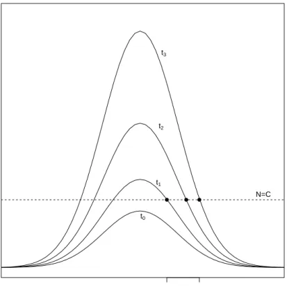
The front propagation method involves calculating the linear spreading velocityv∗, which is the velocity at which arbitrarily small linear perturbations about the unstable state grow and spread, according to the equations obtained by linearising the full model about the unstable steady state (van Saarloos, 2003). This method can be used to determine the long time behaviour of the front which propagates to the right into the unstable steady state. It is therefore preferable to the method described above where an Ansatz of the form N(x, t) = U(x − ct) is made, because that method gives a continuous family of front solutions (van Saarloos, 2003). Fig. 1.1 shows an example of how a typical initial condition grows and spreads in time according to the equations linearised about the unstable steady state (for example, the linearised Fisher equation given in Eqn. (1.4) below). The linear spreading speed is then defined as the asymptotic speed of the point

xC(t):

v∗ ≡ lim

t→∞

dxC(t)

dt

I will now use the example of Eqn. (1.2) to explain how the front propagation method works (this is based on the explanation given in van Saarloos (2003)). Linearising

(23)

xC(t1) xC(t3) N(x,t) x ● ● ● N=C t0 t1 t2 t3

Figure 1.1: Growth and spread of a populationN according to Eqn. (1.4). The curves show the

initial condition N(x, t0) and how the population spreads at successive times. The asymptotic

spreading speedv∗ to the right is defined as the asymptotic speed of the positionsxC(t), where

N(x, t)reaches the dashed lineN =C(shown as the points on this graph). This figure is adapted

(24)

Eqn. (1.2) about the unstable steady stateN = 0gives

∂N

∂t =D

∂2_N

∂x2 +rN. (1.4)

Linearising about the unstable state means that Fourier modes grow for a range of spatial wavenumbersk. This means taking a spatial Fourier transform, so that

˜

N(k, t) =

Z ∞

−∞

N(x, t)e−ikxdx,

and substituting in the Ansatz

˜

N(k, t) = ¯N(k)e−iω(k)t,

gives the dispersion relation ω(k) of Fourier modes of Eqn. (1.4), where N¯(k) is the Fourier transform of the initial conditionN(x, t = 0).

It is then possible to writeN(x, t)fort >0as the inverse Fourier transform

N(x, t) = 1 2π Z ∞ −∞ ¯ N(k)eikx−iω(k)tdk. (1.5) Assuming that the asymptotic spreading speedv∗is finite implies that to look in the frame

ζ = x−v∗t, the right flank is seen neither to grow nor decay exponentially. Then to determinev∗, the inverse Fourier formula Eqn. (1.5), needs to be written in this frame

N(ζ, t) = 1 2π Z ∞ −∞ ¯ N(k)eikζ−i[ω(k)−kv∗]tdk. (1.6)

v∗ can then be determined by analysing when Eqn. (1.6) neither leads to exponential growth nor decay in the limit where ζ is finite and t → ∞. It is not possible to just evaluate the integral by closing the contour in the upper half of the k-plane, because the large-k behaviour of the exponent is dominated by the large-k behaviour of ω(k). However, the large time limit means that a saddle-point approximation can be performed, where the k-contour can be deformed to go through the point in the complex k plane where the term between square brackets in Eqn. (1.6) varies least with k. The integral is then dominated by the contribution from the region near this point, and so the saddle pointk∗ is given by d[ω(k)−v∗k] dk k∗ = 0 ⇒ v∗ = dω(k) dk k∗ . (1.7)

(25)

These equations have solutions in both the upper and lower half of the complexk-plane. Here, I am interested in the right flank, and so look for solutions in the upper half of the plane which correspond to the asymptotic decay towards largexin Eqn. (1.6). If the

k-contour is deformed into the complex plane to go through the saddle point in the upper half plane, then the dominant term of the integral is the exponential factor in Eqn. (1.6) evaluated at the saddle point, so ei[ω(k∗)−v∗k∗]t_{. The requirement that this term neither}

grows nor decays exponentially gives that

=ω(k∗)−v∗=k∗ = 0 ⇒ v∗ = =ω(k

∗₎

=k∗ , (1.8)

where=denotes the imaginary part.

Returning to the example of the Fisher equation, substituting into Eqn. (1.4) the Fourier modeN0eikx−iω(k)t, whereN0is the initial condition, gives

−iω(k)N0eikx−iω(k)t=−Dk2N0eikx−iω(k)t+rN0eikx−iω(k)t.

The Fourier mode cancels throughout, givingω(k)to be

ω(k) = i(r−Dk2).

v∗ can then be calculated using Eqns. (1.7) and (1.8). Firstk∗ needs to be calculated, this can be done by letting k∗ = x+iy, wherex andy are real numbers to be determined. This gives that

ω(k∗) =i(r−Dx2+Dy2−2iDxy),

and using Eqn. (1.7)

v∗ = dω(k) dk k∗ =−2iD(x+iy).

Substituting these into Eqn. (1.8) gives

r−Dx2−Dy2+ 2iDxy = 0.

Both the imaginary and real parts must equal zero, which gives thatx= 0andy=pr D.

This gives thatk∗ = ipr

D and that the linear spreading speed is given byv

∗ _{= 2}√_rD_. For the Fisher equation, the speed at which perturbations about the unstable steady state grow and spread is therefore found to be2√rD.

(26)

1.2.5 Statistical models

The models described above are mechanistic models and explicitly take into account demographic processes. In predicting the response of species to climate change species distribution models can also be used. These models look at the relationship between a species’ current distribution and climate, and use this to predict a species’ future distribution under different climate change scenarios. This approach has limitations, although recent advances have begun to incorporate population dynamics and dispersal (for a discussion of these see Travis and Dytham, 2012). However, as these types of models will not be used in this thesis they will not be discussed further.

1.3

Limits to species’ ranges

All species globally exist in a limited area, known as a species’ ‘range’. In the short term populations cannot become established beyond their range because they have negative growth rates in these new habitats (Bridle and Vines, 2007). However, over long timescales species have adapted to unfavourable conditions. For range margins to form it must therefore be that something is preventing adaptation at the range edge. There are two different explanations for why adaptation fails: (i) adaptation and hence range expansions may be prevented because locally beneficial alleles at the range edge may be limited by Allee effects, genetic drift and a low rate of mutation into these populations; and (ii) continual immigration of locally deleterious alleles into populations at the range edge can swamp locally adapted alleles and so prevent expansion, which is termed gene swamping (reviewed in Bridle and Vines, 2007; Sexton et al., 2009). Examples of theoretical models that have investigated these explanations for the prevention of adaptation at range margins will be discussed below (see Table 1.1 for a summary).

Quantitative trait models have been used to investigate whether gene flow from central to edge populations can result in populations failing to adapt (reviewed in Lenormand, 2002). These models incorporate population ecology and genetics by following changes in the mean of a quantitative trait along a cline, and looking at how range margins are formed along this gradient. The environment changes as a linear function of space and/or time, and so there is an optimum value of the trait at each point along the gradient which maximises survival and reproduction. Using these models it has been shown that at the centre of a species’ range the equilibrium for a trait mean is close to its optimum, but further out towards the range edge the mean increasingly departs from the optimum

(27)

(Garc´ıa-Ramos and Kirkpatrick, 1997). When gene flow from regions of high to low density occurs, adaptation at the periphery is then hampered (Kirkpatrick and Barton, 1997).

In this case one of two scenarios may evolve. If the trait mean matches the optimum for the entire range then the population is adapted everywhere, and so can expand without limit. However, if the environmental gradient is steep then gene swamping of maladapted phenotypes prevents the trait mean from matching the optimum, and so the species has a limited range (Kirkpatrick and Barton, 1997). Competition with other species has been found to increase this effect as competition reduces population densities at the range edge, thus increasing gene swamping from central populations, which can sharpen range edges (Case and Taper, 2000). Other biotic interactions, such as between predators and prey, can also result in the formation of range margins. If predators are effective dispersers then this can increase the effect of gene flow limiting the prey species’ range (Holt et al., 2011).

The form of density dependence used in these models has been found to influence the formation of range margins. If density dependence is strong at high densities then this can reduce the effects of gene swamping (Filin et al., 2008), so that steeper gradients are needed to prevent uniform adaptation than found by Kirkpatrick and Barton (1997) who assume logistic density dependence. However, taking into account demographic stochasticity suggests that the local carrying capacity can have an effect on adaptation at range margins (Bridle et al., 2010), with smaller ranges predicted than those predicted using deterministic models (Kirkpatrick and Barton, 1997).

In these models genetic variance is assumed to be fixed across the entire range, whereas in reality mutation, migration and selection will mean it evolves (Bridle and Vines, 2007). If genetic variance is allowed to evolve then gene flow to peripheral populations is predicted to cause an increase in genetic variance, and so outweigh the effect of gene swamping (Barton, 2001). This allows the species to adapt to a wider range, and so predicts a contrasting effect, that gene flow can rescue peripheral populations. Genetic drift also increases gene flow, which can lower differences in fitness across the range, and so result in higher total fitness (Alleaume-Benharira et al., 2006). Positive effects of immigration on local adaptation are also found if species experience Allee effects as a result of low population densities at the range edge (Holt et al., 2004; Kanarek and Webb, 2010). These models therefore suggest that gene flow can facilitate adaptation and not hinder it, with the amount of genetic variance predicted to be important in determining whether adaptation

(28)

15

Type of model Assumptions Main conclusion of study Reference

Deterministic Type of trait Spatial variation Genetic Population

/stochastic Habitat Environment variance growth

Deterministic Quantitative Continuous Cline Fixed Negative Trait mean close to optimum at centre [1] Fixed in time density- of range, and departs from this as

dependence move to range edge.

Strong density dependence means [2] steeper gradients are needed for

gene flow to prevent adaptation.

Gene flow from central populations [3] can prevent adaptation at the

Varies in time periphery. [4]

Not fixed Gene flow to peripheral populations [4]

Fixed in time causes an increase in genetic [5]

variance, which allows adaptation

Stochastic Patches Fixed in time at range edges. [6]

(29)

16

Deterministic Type of trait Spatial variation Genetic Population

/stochastic Habitat Environment variance growth

bi-allelic Fixed in time adaptation at range margins.

loci

Deterministic Haploid Two Source and sink Allee effects Immigration to peripheral populations [8]

variation patches Fixed in time can increase adaptation if they

Quantitative Continuous Cline Fixed are experiencing Allee effects. [9]

Fixed in time Negative Competitive interactions increase the [10] density- effects of gene flow sharpening

dependence range edges.

Predators can increase the effects of [11] gene flow on limiting prey species’ range.

Not spatially Two niches Resource Competition for limited resources [12] explicit fixed in time dependent results in stable range limits even

and space without gene flow.

References: [1] Garc´ıa-Ramos and Kirkpatrick (1997); [2] Filin et al. (2008); [3] Kirkpatrick and Barton (1997); [4] Polechova et al. (2009); [5] Barton (2001); [6] Alleaume-Benharira et al. (2006); [7] Bridle et al. (2010); [8] Holt et al. (2004); [9] Kanarek and Webb (2010); [10] Case and Taper (2000); [11] Holt et al. (2011); [12] Price and Kirkpatrick (2009).

(30)

occurs at range margins (Bridle et al., 2010; Kanarek and Webb, 2010).

Apart from a failure to adapt to unfavourable conditions, range margins may also be formed as a result of obstacles preventing further dispersal, abrupt changes in the environment or by interactions with other species (Gaston, 2003). Competition between species is considered to be a common process that sets range limits (reviewed in Case et al., 2005). If species compete for limited resources then it is predicted that range limits can be evolutionarily stable in time, even if there is no gene flow disrupting adaptation (Price and Kirkpatrick, 2009).

1.3.1 Empirical evidence of limits to species’ ranges

Many of the theories behind why species have range limits have also been investigated empirically. Sexton et al. (2009) reviewed empirical evidence for the different causes of range limits and determined how much support there is from current studies for each cause. They found that 23 out of 26 studies provided support for the role of competition in setting rage limits. This support has come from correlative approaches, mechanistic models and experimental manipulations. For example, transplantation experiments have shown that in the absence of competition from the barnacle Semibalanus balanoides another barnacleChthamalus fragilis can exist beyond its northern range limit (Wethey, 2002). This suggests that competition between these barnacles is setting the range limit ofC. fragilis.

There is less empirical evidence supporting the theory that a failure to adapt results in species having range limits. However, recent technological and analytical advances have meant that these theories are now easier to test, and so evidence is starting to accumulate. For example, Bridle et al. (2009) have found that the effects of gene flow on local adaptation in rainforestDrosopilacan depend on the steepness of the environmental gradient. The swamping effect of gene flow preventing evolution of cold tolerances was found to occur along a steep altitudinal gradient. However, along a shallower gradient gene flow may have facilitated local adaptation. This study provides evidence to show that under some conditions gene swamping may prevent adaptation at range margins, supporting the predictions of theoretical models (e.g. Bridle et al., 2010; Kirkpatrick and Barton, 1997).

(31)

1.4

Evolution of a species’ range

1.4.1 The speed of range expansions

If marginal conditions change, for example as a result of climate change, then species’ ranges may be able to evolve. Models have shown that the rate of climate change can have an effect on whether species can respond by expanding their range. If the climate changes at a slow enough rate, it is predicted that a species is able to persist and shift its range along the climate gradient (Pease et al., 1989). However, if the rate of environmental change is too fast then the species will become extinct. In a continuously changing environment another model found that the mean phenotype evolves to lag behind the optimum, as the optimum changes with climate. The magnitude of this lag determines whether or not a species becomes extinct (B¨urger and Lynch, 1995). There have been many developments since these early models that also predict there will be a time lag between the climate shifting and the population shifting (e.g. Mustin et al., 2009). However, if species have larger amounts of genetic variation then they are predicted to survive greater rates of environmental change (Duputi´e et al., 2012; Pease et al., 1989; Polechova et al., 2009)

Adaptation to the environment, as previously discussed, has an impact on range expansions (reviewed in Shaw and Etterson, 2012). If range expansions are occurring along environmental gradients then the steeper the gradient, the slower the rate of expansion because there is more maladaptation in the advancing wave front (Garc´ıa-Ramos and Rodr´ıguez, 2002). Climate change may lead to reductions in the steepness of temperature gradients, as temperatures are increasing more towards the poles (Walther et al., 2002). In this case there may be moderate increases in the speed of expansion as faster invasion speeds are observed on shallower gradients (Garc´ıa-Ramos and Rodr´ıguez, 2002).

The size of a species’ range may also affect its ability to respond, as results from stochastic simulations predict that species with broader ranges are more likely to be susceptible to extinction as a result of climate change (Atkins and Travis, 2010). This is because if individuals continue to persist in an area despite their optimum climatic conditions having shifted, they can block locally adapted genotypes and prevent them from expanding their range. If maladapted individuals have higher rates of mortality this weakens the blocking effect (Atkins and Travis, 2010).

(32)

species are able to respond to climate change by expanding their range. Investigations of different patterns of habitat loss on range expansions predict that even if a species survives a period of climate change, the spatial structure of the landscape may mean that it has a new smaller range (McInerny et al., 2007). This is because the arrangement of the landscape in the new climate window may mean that available habitat is not accessible, and so the species can only inhabit part of the landscape. The spatial arrangement of the landscape that benefits static and dynamic range margins may also be different, as it has been predicted that the spatial arrangement that maximises the speed of range expansions is different from the arrangement that maximises species persistence in a static landscape (Hodgson et al., 2012)

Range expansions into areas occupied by a competitor have been found to occur more slowly (Burton et al., 2010), with the type of competition occurring between species having an effect on the evolution of a species’ range. For example, if dispersal increases with population density, a species experiencing contest competition is less likely to persist than a species experiencing scramble competition (Best et al., 2007). Rates of climate change can also have differing effects on species that are mutualists and competitors. A slower rate of climate change favours the persistence of mutualists, whereas with higher rates, competitors out-compete the mutualists and prevent their range from expanding (Brooker et al., 2007). During climate change the nature of species interactions may also be affected. For example, a lack of suitable host plants beyond herbivorous species’ current ranges may restrict range expansions, or the release of natural enemies may promote range expansions as interacting species shift at different rates (Hellmann et al., 2012).

1.4.2 Changing genetic compositions of expanding populations

During range expansions the genetic compositions of populations may change (review see Excoffier et al., 2009), which may either facilitate or hinder range shifting. A low rate of mutation into edge populations, which limits the presence of locally beneficial alleles for adaptation, has been proposed as a mechanism for forming range margins. During range expansions a theory emerging from the literature is that ‘mutation surfing’ can occur (Klopfstein et al., 2006). This is where mutations arising on the edge of a range expansion can sometimes ‘surf’ on the wave of advance (Edmonds et al., 2004). This occurs because occasionally new mutations increase in frequency and spread with the invasion wave, potentially over long distances, and become fixed in the population.

(33)

It is predicted that if neutral (Klopfstein et al., 2006) or beneficial (Hallatschek and Nelson, 2010) mutations surf then beneficial alleles can become fixed at the invasion front, which can increase the rate of evolutionary adaptation of an expanding population. However, other studies have found that non-neutral mutations can also surf leading to high frequencies of deleterious mutations at the range edge. This can mean that instead of increased evolution there is increased mutational load during a range expansion (Hallatschek and Nelson, 2010; Travis et al., 2007).

Other models also suggest that mutations can have an impact on range expansions. In a spatially continuous environment it is predicted that individual mutations that successfully establish often lead to substantial increases in range because they increase adaptation at the range front (Behrman and Kirkpatrick, 2011). Mutations that become established in shallow gradients were found to result in larger range expansions than those that become established in steep gradients. However, if the environment is also changing in time, then there is a limit to the rate of change that allows beneficial mutations to become established (Kirkpatrick and Peischl, 2013). Only below this limit are beneficial mutations able to aid adaptation to a changing environment. Beneficial mutations may therefore result in increased range expansions if they can become established, but deleterious mutations may prevent range expansions.

1.5

Evolution of dispersal

Dispersal is a key trait that will determine whether species’ ranges can evolve, and so will be discussed in more detail now. First, the causes of dispersal evolution will briefly be discussed, followed by a review of the current theoretical and empirical evidence for the evolution of dispersal during range expansions.

Dispersal is any movement of individuals or propagules which has the potential to allow gene flow across space (Ronce, 2007). This encompasses both natal and breeding dispersal. There are three stages that make up dispersal movement: (i) emigration, (ii) a transient stage and (iii) immigration. Dispersal is important because it enables species to be able to persist and evolve (Clobert et al., 2001). Dispersal may evolve when the cost of movement is smaller than the fitness benefit from moving to a new patch (Bowler and Benton, 2005). The costs of dispersal can be either energetic, time, risk or opportunity costs and can occur during any (or all) of the different stages of dispersal movement (review see Bonte et al., 2012).

(34)

1.5.1 Scenarios under which dispersal evolves

The scenarios under which dispersal evolves have been divided into three main categories (Ronce et al., 2001):

• Spatial heterogeneity in habitat quality. If habitat quality differs in space then dispersal enables individuals to arrive or depart from different locations. A species can then choose to become established in a habitat where they may have a higher fitness, a process referred to as habitat selection.

• Temporal heterogeneity in habitat quality. If habitat quality fluctuates over time then dispersal can evolve to escape local extinctions, and may be viewed as a bet-hedging strategy. This is because dispersal distributes offspring from the same parents over different conditions, so increasing the variance in expected fitness.

• Local competition. By dispersing from its natal patch an individual can reduce the strength of competition in the patch. If this occurs dispersal can be thought of as an altruistic trait and its evolution understood using kin selection theory.

Spatial heterogeneity in habitat quality: Different models disagree in whether spatial heterogeneity is required for evolution of dispersal. A simple two patch model predicts that if there are differences in habitat quality, then dispersal will be selected for (McPeek and Holt, 1992). However, inclusion of demographic stochasticity predicts that dispersal can evolve even if there is no spatial variation (Cadet et al., 2003; Travis and Dytham, 1998). Demographic stochasticity has been found to select for intermediate rates of dispersal (Travis and Dytham, 1998). High dispersal is selected against because after dispersal high dispersers are more likely to be in a patch that is above its equilibrium density. Low dispersal is also selected against because these dispersers are less efficient at recolonising patches where they have become extinct.

Patterns of habitat availability affect the rate of dispersal that evolves. Reducing the amount of available habitat results in lower rates of dispersal evolving (Travis and Dytham, 1999). For example, in a fragmented landscape, dispersal propensity of the bog fritillary butterfly,Boloria eunomia, was found to be one order of magnitude lower than in a continuous landscape (Schtickzelle et al., 2006). However, if in a fragmented landscape individuals can distinguish between suitable and unsuitable habitat patches, then a higher rate of dispersal evolves (Heino and Hanski, 2001). There can also be differences in the dispersal strategy that evolves at different points in a species’ range, with lower mean

(35)

dispersal distances often found at the range margin than at the range core (Gros et al., 2006).

Temporal heterogeneity in habitat quality: Models predict that dispersal will be favoured in habitats that are temporally heterogenous (Travis and Dytham, 1999), because if a resource is moving species need to be able to track it. Metapopulation models that investigate evolutionary stable strategies find that when local extinctions occur because of environmental and demographic stochasticity, dispersal is selected for (Comins, 1982; Comins et al., 1980; Levin et al., 1984; Olivieri et al., 1995). It has also been shown using an experimental microcosm that dispersive mutants ofCaenorhabditis elegansincrease in frequency when there are increased rates of patch destruction (Friedenberg, 2003). There are, however, contrasting predictions as incorporation of within-patch dynamics into a metapopulation model suggests that increasing extinction rates may not always lead to the evolution of increased dispersal rates (Ronce et al., 2000).

Local competition: Competitive interactions between relatives have been found to favour positive dispersal rates even if the environment is temporally and spatially constant (Comins, 1982; Comins et al., 1980). It has been demonstrated that there is a threshold population density for which staying and leaving are equally profitable, but above this threshold everybody should leave (Metz and Gyllenberg, 2001; Poethke and Hovestadt, 2002). A generalisation of this model predicts that if there is enough variability in patch types and enough temporal variation as a result of catastrophes, then evolutionary branching of dispersal strategies will occur (Parvinen, 2002). It has been found that offspring increase their dispersal rate in response to the presence of kin in some species. For example, the decision to disperse in response to potential kin competition has been found to occur in lizards (Le Galliard et al., 2003) and fig wasps (Moore et al., 2006).

However, models have not always found kin selection to lead to evolution of dispersal. For example, dispersal rates may decrease rather than increase as a result of kin selection occurring between dispersers that have originated from the same population (Gandon and Michalakis, 1999). Also, if population sizes are small or there is a low deme size, dispersal rate has been found to decrease (Gandon and Rousset, 1999; Travis and Dytham, 1998). If populations experience Allee effects this may result in the dispersal rate evolving to be too low for metapopulations to be able to persist (Rousset and Ronce, 2004). Also, one study suggests that it may in fact be competition with unrelated individuals, rather than the more generally accepted explanation of kin competition, that explains the evolution of dispersal (Jansen and Vitalis, 2007). This has been found to be the case in feral horses,

(36)

where although dispersal from the natal group is affected by kin competition, dispersal from the natal area is affected by the size of non-kin groups (Kaseda et al., 1997).

1.5.2 Evolution of dispersal during range expansions

There is increasing empirical and theoretical evidence that during range expansions evolution of dispersal occurs, as there is selection pressure for increased dispersal during invasions and range expansions. It has been found that faster rates of spread can occur if dispersal evolves during an invasion, with the cost of dispersal determining the rate of expansion that evolves (Travis and Dytham, 2002). The extent to which dispersal evolves during range expansions, and how this results in increased rates of spread, has been found to depend on different factors. Increased levels of evolution have been found to occur if there are no competitors present (Burton et al., 2010; Kubisch et al., 2013), if escape from natural enemies occurs (Phillips et al., 2010b), if Allee effects are absent (Travis and Dytham, 2002), if there is a greater quantity of habitat available (Hughes et al., 2007) and if there are faster rates of climate change (Boeye et al., 2013).

Modelling different dispersal behaviours can also lead to species’ range expansions occurring at different rates. Faster range expansions have been found to occur when dispersal is density dependent (Travis et al., 2009), because dispersal evolves to occur at lower population densities during a range expansion than if dispersal is density-independent. Including more complexity in models so that there is evolution of a dispersal kernel, rather than just of an emigration rate, also results in faster range expansions (Boeye et al., 2013; Phillips et al., 2008; Travis et al., 2010), as does temporal variability of dispersal (Ellner and Schreiber, 2012). This is because fluctuations in the mean dispersal distance generate occasional long distance dispersal events, which result in faster speeds than if the mean dispersal distance was constant over time.

Dispersal behaviour may also evolve during a range expansion. It has been shown that selection favours individual disperser behaviour that increases the rate of range expansion for the population, rather than selecting for behaviour that minimises disperser mortality (Bartoń et al., 2012). Evolution of straighter dispersal trajectories has also been found to result in faster range expansions (Bartoń et al., 2012; Phillips et al., 2008). There is evidence that the increased rates of spread found to be occurring during the invasion of cane toads in Australia (Phillips et al., 2006, 2010a) is partly a result of this change in behaviour (Phillips et al., 2008). Lindström et al. (2013) have quantified this effect and predict that displacement of toads at the invasion front can be twice as far as toads at the

(37)

same site a few years later, which is a result of these toads spending longer time dispersing and having longer, more directed movements when dispersing.

Increasing empirical evidence supports these predictions that evolutionary adaptations related to dispersal ability are occurring in species that are expanding their ranges as a result of climate change (review see Hill et al., 2011). For example, traits related to increased flight ability have been found in more recently colonised sites of the speckled wood butterfly, Pararge aegeria. These sites were found to have populations with larger adults, greater thorax mass and broader thorax shape (Hill et al., 1999a; Hughes et al., 2003, 2007). The cane toad has also been found to have evolution of traits related to dispersal at the front of its range expansion. As well as the toads travelling in straighter lines at the range front (Phillips et al., 2008), these toads have also been found to have longer legs (Phillips et al., 2006) so disperse over longer distances.

1.5.3 Evolution of dispersal along environmental gradients

Most studies discussed so far have looked at range expansions in a homogenous environment. However, most species’ ranges are structured across gradients (Bridges et al., 2007). On a static gradient it has been shown that different dispersal strategies evolve at different positions along a species’ range (Dytham, 2009). Increased dispersal distances are found to evolve at the range margin if there is increased habitat turnover, reduced birth rate and reduced habitat quality, whereas reduced dispersal distances are found if there are increased costs to dispersal (Dytham, 2009). When a shifting environment is introduced then for all types of gradient there is always increased dispersal during range expansions (Kubisch et al., 2010).

Climate change is expected to result in increased environmental stochasticity, which along gradients of dispersal mortality is predicted to result in evolution of increased dispersal (Kubisch et al., 2011). In this case greater range expansions are found to occur if dispersal is density dependent. However, sometimes evolution of increased dispersal can lead to the range overshooting what will be its final position when the environmental conditions have stabilised, which is a result of selection favouring lower dispersal at stable range margins (Kubisch et al., 2010).

If a species expands its range for some time along a homogenous environment before encountering an environmental gradient, then the evolution of increased dispersal can slow adaptation to the gradient, which may hamper (and even stop) range shifting

(38)

(Phillips, 2012). Increased dispersal means that there are more maladapted genes from the homogenous conditions preventing adaptation to the environmental gradient. The extent to which the gradient acts as a barrier depends upon when the environmental gradient is encountered during the range expansion. The earlier during range shifting the gradient is encountered, the less prone to stopping the expansion will be (Phillips, 2012). This is in contrast to the case where instead of encountering a gradient during a range expansion, a species encounters an area of unsuitable habitat. In this case evolution of increased dispersal at the range edge can help a species to overcome this barrier and continue expansion (Travis et al., 2010). When encountering gaps in the landscape more rapid climate change can result in greater dispersal distances evolving, which can again aid range expansions (Boeye et al., 2013).

1.6

Trade-offs between dispersal and other traits

There is evidence, then, that during range expansions there is often selection for evolution of increased dispersal and that this can lead to increased rates of spread. However, not all theoretical studies that look at the evolution of dispersal consider whether increased dispersal will lead to trade-offs in other traits despite lots of empirical evidence for their existence (review see Bonte et al., 2012).

A common trade-off is that more dispersive individuals have reduced fecundity. For example, extreme trade-offs occur in wing polymorphic insects, where one morph is capable of flight and the other is flightless (review see Zera and Denno, 1997). In these insects the morph capable of flight has large functional flight muscles, whereas the flightless morph has small non-functional flight muscles but has much bigger ovaries (Zera and Harshman, 2001). During range expansions it has been found that increased frequencies of the long winged morphs of four species of wing-dimorphic bush crickets were found in recently colonised sites at the range margin (Simmons and Thomas, 2004). However, the impact that these extreme trade-offs between dispersal and reproduction may have on the rate of range expansions is unknown, and so this is a question that I will explore in this thesis.

There is also evidence that the evolution of increased dispersal during range expansions can cause trade-offs. For example, populations at the expanding range margin of the speckled wood butterfly were found to invest more in dispersal at the cost of reduced investment in reproduction (Hughes et al., 2003). This trade-off between dispersal and

(39)

reproductive rate is the most common assumption made in theoretical models (Phillips et al., 2010b). However, there are many other costs associated with increased dispersal (Bonte et al., 2012).

One of the few theoretical studies that investigates trade-offs with other traits during range expansions predicts that increased dispersal at the range front results in decreased investment in competitive ability rather than reduced fecundity (Burton et al., 2010). It has also been suggested that increased dispersal and reproduction may be able to trade-off with other traits not related to fitness at the invasion front, such as defence against natural enemies (Phillips et al., 2010b). Further research is therefore needed to understand how evolution of increased dispersal ability during range expansions may result in trade-offs with other traits. In particular, little is known about how trade-offs may affect range expansions along environmental gradients, and so this will also be investigated in this thesis.

1.7

Outline of thesis

This thesis uses both deterministic and stochastic population-based models to investigate how interactions between dispersal evolution and other traits can influence the formation of range margins and the rates of range expansions.

Chapter 2 uses a deterministic model to look at the invasion of a species that consists of two morphs that exhibit dispersal polymorphism. This study shows that if there are trade-offs in the establishment and dispersal abilities of the two morphs then the presence of both phenotypes can result in faster range expansions than if a single phenotype were present in the population, a phenomenon known as ‘anomalous invasion speeds’. Surprisingly, these speeds were found to persist when the mutation rate between morphs is vanishingly small.

Chapter 3 uses a stochastic model to determine whether the anomalous invasion speeds found in Chapter 2 are observed in a model that incorporates demographic stochasticity. Simulations of this model suggest that anomalous speeds are still found to occur in stochastic models. In this case, anomalous speeds occur when the carrying capacity of the population is high, the mutation rate between morphs is high or the individual morphs have similar invasion speeds.

Chapter 4 is an extension of the model in Chapter 3 to explicitly model a shifting climate. This model is used to investigate whether dispersal polymorphism helps or hinders a

(40)

species’ ability to keep up with climate change. The results suggest that if there is a trade-off between dispersal and establishment then this helps a species to keep up with climate change, but if one morph is superior either in terms of establishment or dispersal then being polymorphic can stop a species keeping up with the rate of climate change.

Chapter 5 uses a quantitative trait model to investigate whether a trade-off between dispersal and adaptation to an environmental gradient can result in the formation of range margins. The results suggest that this trade-off can lead to the formation of range margins with the size of the range determined by the steepness of the environmental gradient, the cost of the trade-off, the size of the phenotypic variance and the strength of stabilising selection. When a shifting gradient was introduced into the model species were then able to expand their ranges.

Chapter 6 is a summary of the results found in this thesis with a discussion of questions for future research that the findings of this work have highlighted. The wider context of this research is discussed with reference to the pressing questions that need to be answered in predicting species’ responses to climate change.

(41)

2. Dispersal polymorphism and the speed of

biological invasions

2.1

Introduction

There is evidence that species are expanding their range as a result of climate change and due to accidental or deliberate introductions of exotic organisms (Hickling et al., 2006; Parmesan and Yohe, 2003; Root et al., 2003; Sakai et al., 2001). The speed at which a species is able to expand its range has important implications for conservation management. Whether a species can shift its range at the same rate as the climate shifts, or whether, and by how much, it lags behind will be important in determining how likely a species is in surviving a period of climate change (Chen et al., 2011; Mustin et al., 2009). The rate of spread of exotic species as a result of introductions can also be important, especially if these species become pests (Ziska et al., 2011).

The speed of a spe