Fast Kernel Classifiers
with Online and Active Learning
Antoine Bordes [email protected]
NEC Laboratories America 4 Independence Way
Princeton, NJ 08540, USA, and
Ecole Sup´erieure de Physique et Chimie Industrielles 10 rue Vauquelin
75231 Paris CEDEX 05, France
Seyda Ertekin [email protected]
The Pennsylvania State University University Park, PA 16802, USA
Jason Weston [email protected]
L´eon Bottou [email protected]
NEC Laboratories America 4 Independence Way Princeton, NJ 08540, USA
Editor: Nello Cristianini
Abstract
Very high dimensional learning systems become theoretically possible when training examples are abundant. The computing cost then becomes the limiting factor. Any efficient learning algorithm should at least take a brief look at each example. But should all examples be given equal attention? This contribution proposes an empirical answer. We first present an online SVM algorithm based on this premise. LASVM yields competitive misclassification rates after a single pass over the training examples, outspeeding state-of-the-art SVM solvers. Then we show how active exam-ple selection can yield faster training, higher accuracies, and simexam-pler models, using only a fraction of the training example labels.
1. Introduction
Electronic computers have vastly enhanced our ability to compute complicated statistical models. Both theory and practice have adapted to take into account the essential compromise between the number of examples and the model capacity (Vapnik, 1998). Cheap, pervasive and networked com-puters are now enhancing our ability to collect observations to an even greater extent. Data sizes outgrow computer speed. During the last decade, processors became 100 times faster, hard disks became 1000 times bigger.
This contribution proposes an empirical answer:
• Section 2 presents kernel classifiers such as Support Vector Machines (SVM). Kernel
classi-fiers are convenient for our purposes because they clearly express their internal states in terms of subsets of the training examples.
• Section 3 proposes a novel online algorithm,LASVM, which converges to the SVM solution.
Experimental evidence on diverse data sets indicates that it reliably reaches competitive ac-curacies after performing a single pass over the training set. It uses less memory and trains significantly faster than state-of-the-art SVM solvers.
• Section 4 investigates two criteria to select informative training examples at each iteration
instead of sequentially processing all examples. Empirical evidence shows that selecting in-formative examples without making use of the class labels can drastically reduce the training time and produce much more compact classifiers with equivalent or superior accuracy.
• Section 5 discusses the above results and formulates theoretical questions. The simplest
ques-tion involves the convergence of these algorithms and is addressed by the appendix. Other questions of greater importance remain open.
2. Kernel Classifiers
Early linear classifiers associate classes y=±1 to patterns x by first transforming the patterns into
feature vectorsΦ(x)and taking the sign of a linear discriminant function:
ˆ
y(x) =w0Φ(x) +b. (1)
The parameters w and b are determined by running some learning algorithm on a set of training
examples (x1,y1)· · ·(xn,yn). The feature function Φ is usually hand chosen for each particular
problem (Nilsson, 1965).
Aizerman et al. (1964) transform such linear classifiers by leveraging two theorems of the Re-producing Kernel theory (Aronszajn, 1950).
The Representation Theorem states that manyΦ-machine learning algorithms produce
parame-ter vectors w that can be expressed as a linear combinations of the training patparame-terns:
w=
n
∑
i=1
αiΦ(xi).
The linear discriminant function (1) can then be written as a kernel expansion
ˆ y(x) =
n
∑
i=1
αiK(x,xi) +b, (2)
where the kernel function K(x,y) represents the dot products Φ(x)0Φ(y) in feature space. This
expression is most useful when a large fraction of the coefficientsαiare zero. Examples such that
αi6=0 are then called Support Vectors.
Mercer’s Theorem precisely states which kernel functions correspond to a dot product for some
corresponding feature functionΦ(x). For instance, the well known RBF kernel K(x,y) =e−γkx−yk2 defines an implicit feature space of infinite dimension.
Kernel classifiers handle such large feature spaces with the comparatively modest computational costs of the kernel function. On the other hand, kernel classifiers must control the decision funcion complexity in order to avoid overfitting the training data in such large feature spaces. This can be achieved by keeping the number of support vectors as low as possible (Littlestone and Warmuth, 1986) or by searching decision boundaries that separate the examples with the largest margin (Vap-nik and Lerner, 1963; Vap(Vap-nik, 1998).
2.1 Support Vector Machines
Support Vector Machines were defined by three incremental steps. First, Vapnik and Lerner (1963) propose to construct the Optimal Hyperplane, that is, the linear classifier that separates the training examples with the widest margin. Then, Guyon, Boser, and Vapnik (1993) propose to construct the Optimal Hyperplane in the feature space induced by a kernel function. Finally, Cortes and Vapnik (1995) show that noisy problems are best addressed by allowing some examples to violate the margin condition.
Support Vector Machines minimize the following objective function in feature space:
min w,b kwk
2+C
∑
ni=1
ξi with
∀i yiyˆ(xi)≥1−ξi
∀i ξi≥0. (3)
For very large values of the hyper-parameter C, this expression minimizeskwk2under the constraint
that all training examples are correctly classified with a margin yiyˆ(xi)greater than 1. Smaller values
of C relax this constraint and produce markedly better results on noisy problems (Cortes and Vapnik, 1995).
In practice this is achieved by solving the dual of this convex optimization problem. The
coef-ficientsαiof the SVM kernel expansion (2) are found by defining the dual objective function
W(α) =
∑
i αiyi−
1
2
∑
i,jαiαjK(xi,xj) (4)and solving the SVM Quadratic Programming (QP) problem:
max
α W(α) with
∑iαi=0 Ai≤αi≤Bi
Ai=min(0,Cyi)
Bi=max(0,Cyi).
(5)
The above formulation slightly deviates from the standard formulation (Cortes and Vapnik, 1995)
because it makes theαicoefficients positive when yi= +1 and negative when yi=−1.
SVMs have been very successful and are very widely used because they reliably deliver state-of-the-art classifiers with minimal tweaking.
Computational Cost of SVMs There are two intuitive lower bounds on the computational cost
1. Suppose that an oracle reveals whetherαi=0 orαi=±C for all i=1. . .n. Computing the
remaining 0<|αi|<C amounts to inverting a matrix of size R×R where R is the number
of support vectors such that 0<|αi|<C. This typically requires a number of operations
proportional to R3.
2. Simply verifying that a vectorα is a solution of the SVM QP problem involves computing
the gradients of W(α)and checking the Karush-Kuhn-Tucker optimality conditions (Vapnik,
1998). With n examples and S support vectors, this requires a number of operations propor-tional to n S.
Few support vectors reach the upper bound C when it gets large. The cost is then dominated by
the R3≈S3. Otherwise the term n S is usually larger. The final number of support vectors therefore
is the critical component of the computational cost of the SVM QP problem.
Assume that increasingly large sets of training examples are drawn from an unknown
distribu-tion P(x,y). Let
B
be the error rate achieved by the best decision function (1) for that distribution.When
B
>0, Steinwart (2004) shows that the number of support vectors is asymptoticallyequiv-alent to 2n
B
. Therefore, regardless of the exact algorithm used, the asymptotical computationalcost of solving the SVM QP problem grows at least like n2 when C is small and n3 when C gets
large. Empirical evidence shows that modern SVM solvers (Chang and Lin, 2001-2004; Collobert and Bengio, 2001) come close to these scaling laws.
Practice however is dominated by the constant factors. When the number of examples grows,
the kernel matrix Ki j=K(xi,xj)becomes very large and cannot be stored in memory. Kernel values
must be computed on the fly or retrieved from a cache of often accessed values. When the cost of computing each kernel value is relatively high, the kernel cache hit rate becomes a major component of the cost of solving the SVM QP problem (Joachims, 1999). Larger problems must be addressed by using algorithms that access kernel values with very consistent patterns.
Section 3 proposes an Online SVM algorithm that accesses kernel values very consistently.
Because it computes the SVM optimum, this algorithm cannot improve on the n2 lower bound.
Because it is an online algorithm, early stopping strategies might give approximate solutions in much shorter times. Section 4 suggests that this can be achieved by carefully choosing which examples are processed at each iteration.
Before introducing the new Online SVM, let us briefly describe other existing online kernel methods, beginning with the kernel Perceptron.
2.2 Kernel Perceptrons
The earliest kernel classifiers (Aizerman et al., 1964) were derived from the Perceptron algorithm (Rosen-blatt, 1958). The decision function (2) is represented by maintaining the set S of the indices i of the support vectors. The bias parameter b remains zero.
Kernel Perceptron
1)
S
← /0, b←0.2) Pick a random example(xt,yt)
3) Compute ˆy(xt) =∑i∈SαiK(xt,xi) +b
4) If ytyˆ(xt) ≤ 0 then
S
←S
∪ {t}, αt ←ytSuch Online Learning Algorithms require very little memory because the examples are pro-cessed one by one and can be discarded after being examined.
Iterations such that ytyˆ(xt)<0 are called mistakes because they correspond to patterns
mis-classified by the perceptron decision boundary. The algorithm then modifies the decision boundary by inserting the misclassified pattern into the kernel expansion. When a solution exists, Novikoff’s Theorem (Novikoff, 1962) states that the algorithm converges after a finite number of mistakes, or equivalently after inserting a finite number of support vectors. Noisy data sets are more problematic.
Large Margin Kernel Perceptrons The success of Support Vector Machines has shown that large classification margins were desirable. On the other hand, the Kernel Perceptron (Section 2.2) makes no attempt to achieve large margins because it happily ignores training examples that are very close to being misclassified.
Many authors have proposed to close the gap with online kernel classifiers by providing larger margins. The Averaged Perceptron (Freund and Schapire, 1998) decision rule is the majority vote of all the decision rules obtained after each iteration of the Kernel Perceptron algorithm. This choice provides a bound comparable to those offered in support of SVMs. Other algorithms (Frieß et al., 1998; Gentile, 2001; Li and Long, 2002; Crammer and Singer, 2003) explicitely construct larger margins. These algorithms modify the decision boundary whenever a training example is either misclassified or classified with an insufficient margin. Such examples are then inserted into the kernel expansion with a suitable coefficient. Unfortunately, this change significantly increases the number of mistakes and therefore the number of support vectors. The increased computational cost and the potential overfitting undermines the positive effects of the increased margin.
Kernel Perceptrons with Removal Step This is why Crammer et al. (2004) suggest an additional step for removing support vectors from the kernel expansion (2). The Budget Perceptron performs very nicely on relatively clean data sets.
Budget Kernel Perceptron (β,N)
1)
S
← /0, b←0.2) Pick a random example(xt,yt)
3) Compute ˆy(xt) =∑i∈SαiK(xt,xi) +b
4) If ytyˆ(xt) ≤ β then,
4a)
S
←S
∪ {t}, αt←yt4b) If |
S
|>N thenS
←S
− {arg maxi∈S yi(yˆ(xi)−αiK(xi,xi))}5) Return to step 2.
Online kernel classifiers usually experience considerable problems with noisy data sets. Each iteration is likely to cause a mistake because the best achievable misclassification rate for such prob-lems is high. The number of support vectors increases very rapidly and potentially causes overfitting and poor convergence. More sophisticated support vector removal criteria avoid this drawback (We-ston et al., 2005). This modified algorithm outperforms all other online kernel classifiers on noisy data sets and matches the performance of Support Vector Machines with less support vectors.
3. Online Support Vector Machines
This section proposes a novel online algorithm namedLASVMthat converges to the SVM solution.
work,LASVMrelies on the traditional “soft margin” SVM formulation, handles noisy data sets, and is nicely related to the SMO algorithm. Experimental evidence on multiple data sets indicates that it reliably reaches competitive test error rates after performing a single pass over the training set. It uses less memory and trains significantly faster than state-of-the-art SVM solvers.
3.1 Quadratic Programming Solvers for SVMs
Sequential Direction Search Efficient numerical algorithms have been developed to solve the SVM QP problem (5). The best known methods are the Conjugate Gradient method (Vapnik, 1982, pages 359–362) and the Sequential Minimal Optimization (Platt, 1999). Both methods work by making successive searches along well chosen directions.
Each direction search solves the restriction of the SVM problem to the half-line starting from the
current vectorαand extending along the specified direction u. Such a search yields a new feasible
vectorα+λ∗u, where
λ∗=arg maxW(α+λu) with 0≤λ≤φ(α,u). (6)
The upper boundφ(α,u)ensures thatα+λu is feasible as well:
φ(α,u) = min
0 if ∑kuk6=0
(Bi−αi)/ui for all i such that ui>0
(Aj−αj)/uj for all j such that uj<0.
(7)
Calculus shows that the optimal value is achieved for
λ∗=min
φ(α,u), ∑igiui
∑i,juiujKi j
(8)
where Ki j=K(xi,xj)and g= (g1. . .gn)is the gradient of W(α), and
gk =
∂W(α)
∂αk = yk−
∑
iαiK(xi,xk) = yk−yˆ(xk) +b. (9)
Sequential Minimal Optimization Platt (1999) observes that direction search computations are much faster when the search direction u mostly contains zero coefficients. At least two coefficients
are needed to ensure that∑kuk=0. The Sequential Minimal Optimization (SMO) algorithm uses
search directions whose coefficients are all zero except for a single+1 and a single−1.
Practical implementations of the SMO algorithm (Chang and Lin, 2001-2004; Collobert and
Bengio, 2001) usually rely on a small positive toleranceτ>0. They only select directions u such
thatφ(α,u)>0 and u0g>τ. This means that we can move along direction u without immediately
reaching a constraint and increase the value of W(α). Such directions are defined by the so-called
τ-violating pair(i,j):
(i,j)is aτ-violating pair ⇐⇒
αi<Bi αj>Aj
SMO Algorithm
1) Setα←0 and compute the initial gradient g (equation 9)
2) Choose aτ-violating pair(i,j). Stop if no such pair exists.
3) λ←min
gi−gj
Kii+Kj j−2Ki j
,Bi−αi,αj−Aj
αi←αi+λ, αj←αj−λ
gs←gs−λ(Kis−Kjs) ∀s∈ {1. . .n}
4) Return to step (2)
The above algorithm does not specify how exactly the τ-violating pairs are chosen. Modern
implementations of SMO select theτ-violating pair(i,j)that maximizes the directional gradient u0g.
This choice was described in the context of Optimal Hyperplanes in both (Vapnik, 1982, pages 362– 364) and (Vapnik et al., 1984).
Regardless of how exactly theτ-violating pairs are chosen, Keerthi and Gilbert (2002) assert
that the SMO algorithm stops after a finite number of steps. This assertion is correct despite a slight flaw in their final argument (Takahashi and Nishi, 2003).
When SMO stops, noτ-violating pair remain. The correspondingαis called aτ-approximate
solution. Proposition 13 in appendix A establishes that such approximate solutions indicate the
location of the solution(s) of the SVM QP problem when the toleranceτbecome close to zero.
3.2 OnlineLASVM
This section presents a novel online SVM algorithm namedLASVM. There are two ways to view
this algorithm.LASVMis an online kernel classifier sporting a support vector removal step: vectors
collected in the current kernel expansion can be removed during the online process.LASVMalso is
a reorganization of the SMO sequential direction searches and, as such, converges to the solution of the SVM QP problem.
Compared to basic kernel perceptrons (Aizerman et al., 1964; Freund and Schapire, 1998), the LASVMalgorithm features a removal step and gracefully handles noisy data. Compared to kernel
perceptrons with removal steps (Crammer et al., 2004; Weston et al., 2005),LASVMconverges to the
known SVM solution. Compared to a traditional SVM solver (Platt, 1999; Chang and Lin,
2001-2004; Collobert and Bengio, 2001),LASVM brings the computational benefits and the flexibility
of online learning algorithms. Experimental evidence indicates that LASVM matches the SVM
accuracy after a single sequential pass over the training examples.
This is achieved by alternating two kinds of direction searches namedPROCESS and
REPRO-CESS. Each direction search involves a pair of examples. Direction searches of thePROCESSkind involve at least one example that is not a support vector of the current kernel expansion. They po-tentially can change the coefficient of this example and make it a support vector. Direction searches
of theREPROCESSkind involve two examples that already are support vectors in the current kernel
expansion. They potentially can zero the coefficient of one or both support vectors and thus remove them from the kernel expansion.
Building Blocks TheLASVMalgorithm maintains three essential pieces of information: the set
S
of potential support vector indices, the coefficientsαi of the current kernel expansion, and theThe coefficient αi are assumed to be null if i∈/
S
. On the other hand, setS
might contain a fewindices i such thatαi=0.
The two basic operations of the OnlineLASVM algorithm correspond to steps 2 and 3 of the
SMO algorithm. These two operations differ from each other because they have different ways to selectτ-violating pairs.
The first operation,PROCESS, attempts to insert example k∈/
S
into the set of current supportvectors. In the online setting this can be used to process a new example at time t. It first adds
example k∈/
S
intoS
(step 1-2). Then it searches a second example inS
to find theτ-violating pairwith maximal gradient (steps 3-4) and performs a direction search (step 5).
LASVM PROCESS(k)
1) Bail out if k∈
S
.2) αk←0 , gk←yk−∑s∈SαsKks,
S
←S
∪ {k}3) If yk= +1 then
i←k , j←arg mins∈Sgs with αs>As
else
j←k , i←arg maxs∈Sgs with αs<Bs
4) Bail out if(i,j)is not aτ-violating pair.
5) λ←min
gi−gj
Kii+Kj j−2Ki j
,Bi−αi,αj−Aj
αi←αi+λ, αj←αj−λ
gs←gs−λ(Kis−Kjs) ∀s∈
S
The second operation, REPROCESS, removes some elements from
S
. It first searches theτ-violating pair of elements of
S
with maximal gradient (steps 1-2), and performs a direction search(step 3). Then it removes blatant non support vectors (step 4). Finally it computes two useful
quantities: the bias term b of the decision function (2) and the gradientδof the mostτ-violating pair
in
S
.LASVM REPROCESS
1) i←arg maxs∈Sgs with αs<Bs
j←arg mins∈Sgs with αs>As
2) Bail out if(i,j)is not aτ-violating pair.
3) λ←min
gi−gj
Kii+Kj j−2Ki j
,Bi−αi,αj−Aj
αi←αi+λ, αj←αj−λ
gs←gs−λ(Kis−Kjs) ∀s∈
S
4) i←arg maxs∈Sgs with αs<Bs
j←arg mins∈Sgs with αs>As
For all s∈
S
such thatαs=0If ys=−1 and gs≥gi then
S
=S
− {s}If ys= +1 and gs≤gj then
S
=S
− {s}Online LASVM After initializing the state variables (step 1), the Online LASVM algorithm
al-ternatesPROCESSandREPROCESSa predefined number of times (step 2). Then it simplifies the
kernel expansion by runningREPROCESSto remove allτ-violating pairs from the kernel expansion
(step 3).
LASVM
1) Initialization:
Seed
S
with a few examples of each class.Setα←0 and compute the initial gradient g (equation 9)
2) Online Iterations:
Repeat a predefined number of times:
- Pick an example kt
- RunPROCESS(kt).
- RunREPROCESSonce.
3) Finishing:
RepeatREPROCESSuntilδ≤τ.
LASVM can be used in the online setup where one is given a continuous stream of fresh random
examples. The online iterations process fresh training examples as they come.LASVMcan also be
used as a stochastic optimization algorithm in the offline setup where the complete training set is available before hand. Each iteration randomly picks an example from the training set.
In practice we run theLASVM online iterations in epochs. Each epoch sequentially visits all
the randomly shuffled training examples. After a predefined number P of epochs, we perform the
finishing step. A single epoch is consistent with the use ofLASVM in the online setup. Multiple
epochs are consistent with the use ofLASVMas a stochastic optimization algorithm in the offline
setup.
Convergence of the Online Iterations Let us first ignore the finishing step (step 3) and assume
that online iterations (step 2) are repeated indefinitely. Suppose that there are remainingτ-violating
pairs at iteration T .
a.) If there areτ-violating pairs(i,j)such that i∈
S
and j∈S
, one of them will be exploited bythe nextREPROCESS.
b.) Otherwise, if there areτ-violating pairs(i,j)such that i∈
S
or j∈S
, each subsequentPRO-CESShas a chance to exploit one of them. The interveningREPROCESSdo nothing because
they bail out at step 2.
c.) Otherwise, allτ-violating pairs involve indices outside
S
. Subsequent calls toPROCESSandREPROCESSbail out until we reach a time t >T such that kt =i and kt+1= j for someτ
-violating pair (i,j). The firstPROCESS then inserts i into
S
and bails out. The followingREPROCESSbails out immediately. Finally the secondPROCESSlocates pair(i,j).
This case is not important in practice. There usually is a support vector s∈
S
such thatAs<αs<Bs. We can then write gi−gj = (gi−gs) + (gs−gj)≤2τand conclude that we
The LASVM online iterations therefore work like the SMO algorithm. Remainingτ-violating
pairs is sooner or later exploited by eitherPROCESS orREPROCESS. As soon as a τ-approximate
solution is reached, the algorithm stops updating the coefficientsα. Theorem 18 in the appendix
gives more precise convergence results for this stochastic algorithm.
The finishing step (step 3) is only useful when one limits the number of online iterations. Run-ningLASVMusually consists in performing a predefined number P of epochs and running the fin-ishing step. Each epoch performs n online iterations by sequentially visiting the randomly shuffled training examples. Empirical evidence suggests indeed that a single epoch yields a classifier almost as good as the SVM solution.
Computational Cost ofLASVM BothPROCESSandREPROCESSrequire a number of operations
proportional to the number S of support vectors in set
S
. Performing P epochs of online iterationsrequires a number of operations proportional to n P ¯S. The average number ¯S of support vectors
scales no more than linearly with n because each online iteration brings at most one new support
vector. The asymptotic cost therefore grows like n2at most. The finishing step is similar to running
a SMO solver on a SVM problem with only S training examples. We recover here the n2 to n3
behavior of standard SVM solvers.
Online algorithms access kernel values with a very specific pattern. Most of the kernel values
accessed byPROCESSandREPROCESSinvolve only support vectors from set
S
. OnlyPROCESSon a new example xkt accesses S fresh kernel values K(xkt,xi)for i∈
S
.Implementation Details Our LASVM implementation reorders the examples after every PRO-CESS or REPROCESS to ensure that the current support vectors come first in the reordered list of indices. The kernel cache records truncated rows of the reordered kernel matrix. SVMLight
(Joachims, 1999) andLIBSVM(Chang and Lin, 2001-2004) also perform such reorderings, but do
so rather infrequently (Joachims, 1999). The reordering overhead is acceptable during the online iterations because the computation of fresh kernel values takes much more time.
Reordering examples during the finishing step was more problematic. We eventually deployed
an adaptation of the shrinking heuristic (Joachims, 1999) for the finishing step only. The set
S
ofsupport vectors is split into an active set Saand an inactive set Si. All support vectors are initially
active. TheREPROCESSiterations are restricted to the active set Saand do not perform any
reorder-ing. About every 1000 iterations, support vectors that hit the boundaries of the box constraints are
either removed from the set
S
of support vectors or moved from the active setS
ato the inactive setS
i. When allτ-violating pairs of the active set are exhausted, the inactive set examples aretrans-ferred back into the active set. The process continues as long as the merged set containsτ-violating
pairs.
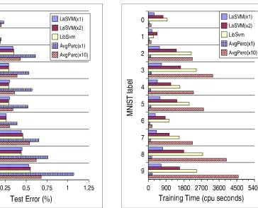
3.3 MNIST Experiments
The OnlineLASVM was first evaluated on the MNIST1 handwritten digit data set (Bottou et al.,
1994). Computing kernel values for this data set is relatively expensive because it involves dot products of 784 gray level pixel values. In the experiments reported below, all algorithms use the same code for computing kernel values. The ten binary classification tasks consist of separating
each digit class from the nine remaining classes. All experiments use RBF kernels withγ=0.005
Figure 1: Compared test error rates for the ten MNIST binary classifiers.
Figure 2: Compared training times for the ten MNIST binary classifiers.
and the same training parameters C=1000 andτ=0.001. Unless indicated otherwise, the kernel
cache size is 256MB.
LASVM versus Sequential Minimal Optimization Baseline results were obtained by running
the state-of-the-art SMO solverLIBSVM (Chang and Lin, 2001-2004). The resulting classifier
ac-curately represents the SVM solution.
Two sets of results are reported forLASVM. TheLASVM×1 results were obtained by performing
a single epoch of online iterations: each training example was processed exactly once during a
single sequential sweep over the training set. TheLASVM×2 results were obtained by performing
two epochs of online iterations.
Figures 1 and 2 show the resulting test errors and training times. LASVM×1 runs about three
times faster thanLIBSVM and yields test error rates very close to the LIBSVM results. Standard
paired significance tests indicate that these small differences are not significant.LASVM×2 usually
runs faster thanLIBSVMand very closely tracks theLIBSVMtest errors.
Neither theLASVM×1 orLASVM×2 experiments yield the exact SVM solution. On this data
Algorithm Error Time
LIBSVM 1.36% 17400s LASVM×1 1.42% 4950s
LASVM×2 1.36% 12210s
Figure 3: Training time as a function of the number of support vectors.
Figure 4: Multiclass errors and training times for the MNIST data set.
Figure 5: Compared numbers of support vec-tors for the ten MNIST binary clas-sifiers.
Figure 6: Training time variation as a
func-tion of the cache size. Relative
changes with respect to the 1GB LIBSVMtimes are averaged over all ten MNIST classifiers.
enough to hold all the dot products involving support vectors. Yet the overall optimization times are
not competitive with those achieved byLIBSVM.
Figure 3 shows the training time as a function of the final number of support vectors for the
ten binary classification problems. BothLIBSVMandLASVM×1 show a linear dependency. The
Figure 4 shows the multiclass error rates and training times obtained by combining the ten
classifiers using the well known 1-versus-rest scheme (Sch¨olkopf and Smola, 2002). LASVM×1
provides almost the same accuracy with much shorter training times. LASVM×2 reproduces the
LIBSVMaccuracy with slightly shorter training time.
Figure 5 shows the resulting number of support vectors. A single epoch of the OnlineLASVM
algorithm gathers most of the support vectors of the SVM solution computed byLIBSVM. The first
iterations of the Online LASVMmight indeed ignore examples that later become support vectors.
Performing a second epoch captures most of the missing support vectors.
LASVMversus the Averaged Perceptron The computational advantage ofLASVMrelies on its apparent ability to match the SVM accuracies after a single epoch. Therefore it must be compared with algorithms such as the Averaged Perceptron (Freund and Schapire, 1998) that provably match
well known upper bounds on the SVM accuracies. TheAVGPERC×1 results in Figures 1 and 2 were
obtained after running a single epoch of the Averaged Perceptron. Although the computing times are
very good, the corresponding test errors are not competitive with those achieved by eitherLIBSVM
orLASVM. Freund and Schapire (1998) suggest that the Averaged Perceptron approaches the actual SVM accuracies after 10 to 30 epochs. Doing so no longer provides the theoretical guarantees. The AVGPERC×10 results in Figures 1 and 2 were obtained after ten epochs. Test error rates indeed approach the SVM results. The corresponding training times are no longer competitive.
Impact of the Kernel Cache Size These training times stress the importance of the kernel cache
size. Figure 2 shows how theAVGPERC×10 runs much faster on problems 0, 1, and 6. This is
hap-pening because the cache is large enough to accomodate the dot products of all examples with all support vectors. Each repeated iteration of the Average Perceptron requires very few additional ker-nel evaluations. This is much less likely to happen when the training set size increases. Computing times then increase drastically because repeated kernel evaluations become necessary.
Figure 6 compares how theLIBSVMandLASVM×1 training times change with the kernel cache
size. The vertical axis reports the relative changes with respect toLIBSVM with one gigabyte of
kernel cache. These changes are averaged over the ten MNIST classifiers. The plot shows how LASVMtolerates much smaller caches. On this problem, LASVM with a 8MB cache runs slightly faster thanLIBSVMwith a 1024MB cache.
Useful orders of magnitude can be obtained by evaluating how large the kernel cache must be to avoid the systematic recomputation of dot-products. Following the notations of Section 2.1, let n
be the number of examples, S be the number of support vectors, and R≤S the number of support
vectors such that 0<|αi|<C.
• In the case ofLIBSVM, the cache must accommodate about n R terms: the examples selected
for the SMO iterations are usually chosen among the R free support vectors. Each SMO iteration needs n distinct dot-products for each selected example.
• To perform a singleLASVMepoch, the cache must only accommodate about S R terms: since
the examples are visited only once, the dot-products computed by aPROCESSoperation can
only be reutilized by subsequent REPROCESS operations. The examples selected by
• To perform multiple LASVM epochs, the cache must accommodate about n S terms: the dot-products computed by processing a particular example are reused when processing the same example again in subsequent epochs. This also applies to multiple Averaged Perceptron epochs.
An efficient single epoch learning algorithm is therefore very desirable when one expects S to be much smaller than n. Unfortunately, this may not be the case when the data set is noisy. Section 3.4 presents results obtained in such less favorable conditions. Section 4 then proposes an active learning method to contain the growth of the number of support vectors, and recover the full benefits of the online approach.
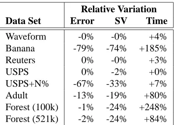
3.4 Multiple Data Set Experiments
Further experiments were carried out with a collection of standard data sets representing diverse noise conditions, training set sizes, and input dimensionality. Figure 7 presents these data sets and the parameters used for the experiments.
Kernel computation times for these data sets are extremely fast. The data either has low di-mensionality or can be represented with sparse vectors. For instance, computing kernel values for two Reuters documents only involves words common to both documents (excluding stop words). The Forest experiments use a kernel implemented with hand optimized assembly code (Graf et al., 2005).
Figure 8 compares the solutions returned byLASVM×1 andLIBSVM. TheLASVM×1
experi-ments call the kernel function much less often, but do not always run faster. The fast kernel
com-putation times expose the relative weakness of our kernel cache implementation. TheLASVM×1
accuracies are very close to the LIBSVM accuracies. The number of support vectors is always
slightly smaller.
LASVM×1 essentially achieves consistent results over very diverse data sets, after performing
one single epoch over the training set only. In this situation, theLASVM PROCESSfunction gets
only once chance to take a particular example into the kernel expansion and potentially make it a support vector. The conservative strategy would be to take all examples and sort them out during
the finishing step. The resulting training times would always be worse than LIBSVM’s because
the finishing step is itself a simplified SMO solver. ThereforeLASVMonline iterations are able to
very quickly discard a large number of examples with a high confidence. This process is not perfect
because we can see that theLASVM×1 number of support vectors are smaller thanLIBSVM’s. Some
good support vectors are discarded erroneously.
Train Size Test Size γ C Cache τ Notes
Waveform1 4000 1000 0.05 1 40M 0.001 Artificial data, 21 dims.
Banana1 4000 1300 0.5 316 40M 0.001 Artificial data, 2 dims. Reuters2 7700 3299 1 1 40M 0.001 Topic “moneyfx” vs. rest. USPS3 7329 2000 2 1000 40M 0.001 Class “0” vs. rest. USPS+N3 7329 2000 2 10 40M 0.001 10% training label noise. Adult3 32562 16282 0.005 100 40M 0.001 As in (Platt, 1999).
Forest3(100k) 100000 50000 1 3 512M 0.001 As in (Collobert et al., 2002). Forest3(521k) 521012 50000 1 3 1250M 0.01 As in (Collobert et al., 2002).
1http://mlg.anu.edu.au/∼raetsch/data/index.html
2http://www.daviddlewis.com/resources/testcollections/reuters21578
3ftp://ftp.ics.uci.edu/pub/machine-learning-databases
Figure 7: Data Sets discussed in Section 3.4.
LIBSVM LASVM×1
Data Set Error SV KCalc Time Error SV KCalc Time
Waveform 8.82% 1006 4.2M 3.2s 8.68% 948 2.2M 2.7s
Banana 9.96% 873 6.8M 9.9s 9.98% 869 6.7M 10.0s
Reuters 2.76% 1493 11.8M 24s 2.76% 1504 9.2M 31.4s
USPS 0.41% 236 1.97M 13.5s 0.43% 201 1.08M 15.9s
USPS+N 0.41% 2750 63M 305s 0.53% 2572 20M 178s
Adult 14.90% 11327 1760M 1079s 14.94% 11268 626M 809s Forest (100k) 8.03% 43251 27569M 14598s 8.15% 41750 18939M 10310s Forest (521k) 4.84% 124782 316750M 159443s 4.83% 122064 188744M 137183s
Figure 8: Comparison ofLIBSVMversusLASVM×1: Test error rates (Error), number of support
vectors (SV), number of kernel calls (KCalc), and training time (Time). Bold characters indicate significative differences.
Relative Variation
Data Set Error SV Time
Waveform -0% -0% +4%
Banana -79% -74% +185%
Reuters 0% -0% +3%
USPS 0% -2% +0%
USPS+N% -67% -33% +7%
Adult -13% -19% +80%
Forest (100k) -1% -24% +248% Forest (521k) -2% -24% +84%
3.5 The Collection of Potential Support Vectors
The final step of theREPROCESSoperation computes the current value of the kernel expansion bias
b and the stopping criterionδ:
gmax=max
s∈S gs withαs<Bs b=
gmax+gmin 2 gmin=min
s∈S gs withαs>As δ=gmax−gmin.
(10)
The quantities gminand gmaxcan be interpreted as bounds for the decision threshold b. The quantity
δthen represents an uncertainty on the decision threshold b.
The quantityδalso controls howLASVMcollects potential support vectors. The definition of
PROCESSand the equality (9) indicate indeed that PROCESS(k) adds the support vector xk to the
kernel expansion if and only if
ykyˆ(xk)<1+ δ
2−τ. (11)
Whenαis optimal, the uncertaintyδis zero, and this condition matches the Karush-Kuhn-Tucker
condition for support vectors ykyˆ(xk)≤1.
Intuitively, relation (11) describes howPROCESScollects potential support vectors that are
com-patible with the current uncertainty levelδ on the threshold b. Simultaneously, the REPROCESS
operations reduceδand discard the support vectors that are no longer compatible with this reduced
uncertainty.
The online iterations of theLASVMalgorithm make equal numbers of PROCESSand
REPRO-CESS for purely heuristic reasons. Nothing guarantees that this is the optimal proportion. The
results reported in Figure 9 clearly suggest to investigate this arbitrage more closely.
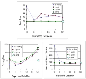
Variations onREPROCESS Experiments were carried out with a slightly modifiedLASVM
al-gorithm: instead of performing a singleREPROCESS, the modified online iterations repeatedly run
REPROCESSuntil the uncertaintyδbecomes smaller than a predefined thresholdδmax.
Figure 10 reports comparative results for the “Banana” data set. Similar results were obtained with other data sets. The three plots report test error rates, training time, and number of support
vectors as a function ofδmax. These measurements were performed after one epoch of online
it-erations without finishing step, and after one and two epochs followed by the finishing step. The
correspondingLIBSVMfigures are indicated by large triangles on the right side of the plot.
Regardless ofδmax, the SVM test error rate can be replicated by performing two epochs followed
by a finishing step. However, this does not guarantee that the optimal SVM solution has been reached.
Large values ofδmaxessentially correspond to the unmodifiedLASVMalgorithm. Small values
ofδmaxconsiderably increases the computation time because each online iteration callsREPROCESS
many times in order to sufficiently reduceδ. Small values ofδmaxalso remove theLASVMability
to produce a competitive result after a single epoch followed by a finishing step. The additional optimization effort discards support vectors more aggressively. Additional epochs are necessary to recapture the support vectors that should have been kept.
There clearly is a sweet spot aroundδmax=3 when one epoch of online iterations alone almost
match the SVM performance and also makes the finishing step very fast. This sweet spot is difficult
Figure 10: Impact of additional REPROCESS measured on “Banana” data set. During the LASVM online iterations, calls toREPROCESSare repeated untilδ<δmax.
bit too large, the algorithm behaves like the unmodifiedLASVM. Short of a deeper understanding
of these effects, the unmodifiedLASVMseems to be a robust compromise.
SimpleSVM The right side of each plot in Figure 10 corresponds to an algorithm that optimizes the coefficient of the current support vectors at each iteration. This is closely related to the
Sim-pleSVM algorithm (Vishwanathan et al., 2003). BothLASVMand the SimpleSVM update a current
kernel expansion by adding or removing one or two support vectors at each iteration. The two key differences are the numerical objective of these updates and their computational costs.
Whereas each SimpleSVM iteration seeks the optimal solution of the SVM QP problem
re-stricted to the current set of support vectors, theLASVMonline iterations merely attempt to improve
the value of the dual objective function W(α). As a a consequence,LASVMneeds a finishing step
and the SimpleSVM does not. On the other hand, Figure 10 suggests that seeking the optimum at each iteration discards support vectors too aggressively to reach competitive accuracies after a single epoch.
Each SimpleSVM iteration updates the current kernel expansion using rank 1 matrix updates (Cauwenberghs and Poggio, 2001) whose computational cost grows as the square of the number of
linearly with the number of examples. Rank 1 updates make good sense when one seeks the optimal coefficients. On the other hand, all the kernel values involving support vectors must be stored in
memory. TheLASVMdirection searches are more amenable to caching strategies for kernel values.
4. Active Selection of Training Examples
The previous section presents LASVM as an Online Learning algorithm or as a Stochastic
Opti-mization algorithm. In both cases, the LASVM online iterations pick random training examples.
The current section departs from this framework and investigates more refined ways to select an informative example for each iteration.
This departure is justified in the offline setup because the complete training set is available beforehand and can be searched for informative examples. It is also justified in the online setup when the continuous stream of fresh training examples is too costly to process, either because the computational requirements are too high, or because it is inpractical to label all the potential training examples.
In particular, we show that selecting informative examples yields considerable speedups. Fur-thermore, training example selection can be achieved without the knowledge of the training example labels. In fact, excessive reliance on the training example labels can have very detrimental effects.
4.1 Gradient Selection
The most obvious approach consists in selecting an example k such that thePROCESS operation
results in a large increase of the dual objective function. This can be approximated by choosing the
example which yields theτ-violating pair with the largest gradient. Depending on the class yk, the
PROCESS(k) operation considers pair(k,j)or(i,k)where i and j are the indices of the examples in
S
with extreme gradients:i=arg max
s∈S
gs withαs<Bs, j=arg min
s∈S
gs withαs>As.
The corresponding gradients are gk−gj for positive examples and gi−gk for negative examples.
Using the expression (9) of the gradients and the value of b andδ computed during the previous
REPROCESS(10), we can write:
when yk= +1, gk−gj=ykgk−
gi+gj
2 +
gi−gj
2 =1+
δ
2−ykyˆ(xk)
when yk=−1, gi−gk=
gi+gj
2 +
gi−gj
2 +ykgk=1+
δ
2−ykyˆ(xk).
This expression shows that the Gradient Selection Criterion simply suggests to pick the most mis-classified example
kG = arg min
k∈/S
ykyˆ(xk). (12)
4.2 Active Selection
When training example labels are unreliable, a conservative approach chooses the example kA
that yields the strongest minimax gradient:
kA = arg min
k∈/S
max
y=±1 y ˆy(xk) = arg mink∈/S |yˆ(xk)|. (13)
This Active Selection Criterion simply chooses the example that comes closest to the current
deci-sion boundary. Such a choice yields a gradient approximatively equal to 1+δ/2 regardless of the
true class of the example.
Criterion (13) does not depend on the labels yk. The resulting learning algorithm only uses the
labels of examples that have been selected during the previous online iterations. This is related to the Pool Based Active Learning paradigm (Cohn et al., 1990).
Early active learning literature, also known as Experiment Design (Fedorov, 1972), contrasts
the passive learner, who observes examples(x,y), with the active learner, who constructs queries x
and observes their labels y. In this setup, the active learner cannot beat the passive learner because he lacks information about the input pattern distribution (Eisenberg and Rivest, 1990). Pool-based active learning algorithms observe the pattern distribution from a vast pool of unlabelled examples.
Instead of constructing queries, they incrementally select unlabelled examples xk and obtain their
labels ykfrom an oracle.
Several authors (Campbell et al., 2000; Schohn and Cohn, 2000; Tong and Koller, 2000) propose incremental active learning algorithms that clearly are related to Active Selection. The initialization consists of obtaining the labels for a small random subset of examples. A SVM is trained using all the labelled examples as a training set. Then one searches the pool for the unlabelled example that comes closest to the SVM decision boundary, one obtains the label of this example, retrains the SVM and reiterates the process.
4.3 Randomized Search
Both criteria (12) and (13) suggest a search through all the training examples. This is impossible in the online setup and potentially expensive in the offline setup.
It is however possible to locate an approximate optimum by simply examining a small constant number of randomly chosen examples. The randomized search first samples M random training
examples and selects the best one among these M examples. With probability 1−ηM, the value
of the criterion for this example exceeds the η-quantile of the criterion for all training examples
(Sch¨olkopf and Smola, 2002, theorem 6.33) regardless of the size of the training set. In practice this means that the best among 59 random training examples has 95% chances to belong to the best 5% examples in the training set.
Randomized search has been used in the offline setup to accelerate various machine learning algorithms (Domingo and Watanabe, 2000; Vishwanathan et al., 2003; Tsang et al., 2005). In the online setup, randomized search is the only practical way to select training examples. For instance,
here is a modification of the basicLASVMalgorithm to select examples using the Active Selection
LASVM+ Active Example Selection + Randomized Search 1) Initialization:
Seed
S
with a few examples of each class.Setα←0 and g←0.
2) Online Iterations:
Repeat a predefined number of times:
- Pick M random examples s1. . .sM.
- kt←arg min
i=1...M
|yˆ(xsi)|
- RunPROCESS(kt).
- RunREPROCESSonce.
3) Finishing:
RepeatREPROCESSuntilδ≤τ.
Each online iteration of the above algorithm is about M times more computationally
expen-sive that an online iteration of the basic LASVMalgorithm. Indeed one must compute the kernel
expansion (2) for M fresh examples instead of a single one (9). This cost can be reduced by heuris-tic techniques for adapting M to the current conditions. For instance, we present experimental
results where one stops collecting new examples as soon as
M
contains five examples such that|yˆ(xs)|<1+δ/2.
Finally the last two paragraphs of appendix A discuss the convergence ofLASVMwith example
selection according to the gradient selection criterion or the active selection criterion. The gradient selection criterion always leads to a solution of the SVM problem. On the other hand, the active selection criterion only does so when one uses the sampling method. In practice this convergence occurs very slowly. The next section presents many reasons to prefer the intermediate kernel classi-fiers visited by this algorithm.
4.4 Example Selection for Online SVMs
This section experimentally compares the LASVM algorithm using different example selection
methods. Four different algorithms are compared:
• RANDOMexample selection randomly picks the next training example among those that have
not yet been PROCESSed. This is equivalent to the plain LASVM algorithm discussed in
Section 3.2.
• GRADIENTexample selection consists in sampling 50 random training examples among those
that have not yet beenPROCESSed. The sampled example with the smallest ykyˆ(xk)is then
selected.
• ACTIVEexample selection consists in sampling 50 random training examples among those
that have not yet beenPROCESSed. The sampled example with the smallest |ˆy(xk)|is then
selected.
• AUTOACTIVEexample selection attempts to adaptively select the sampling size. Sampling
stops as soon as 5 examples are within distance 1+δ/2 of the decision boundary. The
max-imum sample size is 100 examples. The sampled example with the smallest|yˆ(xk)|is then
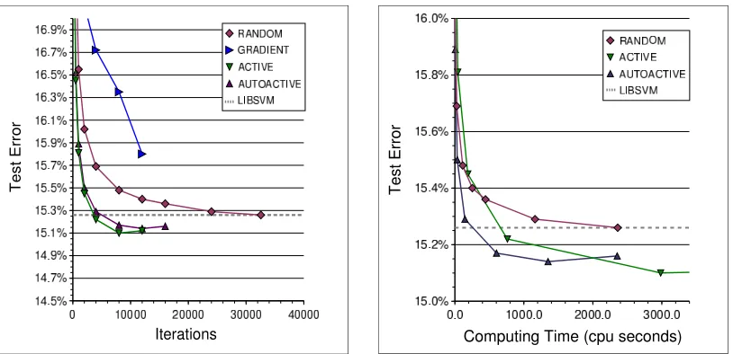
Figure 11: Comparing example selection criteria on the Adult data set. Measurements were per-formed on 65 runs using randomly selected training sets. The graphs show the error measured on the remaining testing examples as a function of the number of iterations
and the computing time. The dashed line represents the LIBSVM test error under the
same conditions.
Adult Data Set We first report experiments performed on the “Adult” data set. This data set provides a good indication of the relative performance of the Gradient and Active selection criteria under noisy conditions.
Reliable results were obtained by averaging experimental results measured for 65 random splits of the full data set into training and test sets. Paired tests indicate that test error differences of 0.25% on a single run are statistically significant at the 95% level. We conservatively estimate that average
error differences of 0.05% are meaningful.
Figure 11 reports the average error rate measured on the test set as a function of the number of online iterations (left plot) and of the average computing time (right plot). Regardless of the
training example selection method, all reported results were measured after performing theLASVM
finishing step. More specifically, we run a predefined number of online iterations, save theLASVM
state, perform the finishing step, measure error rates and number of support vectors, and restore the
savedLASVM state before proceeding with more online iterations. Computing time includes the
duration of the online iterations and the duration of the finishing step.
The GRADIENT example selection criterion performs very poorly on this noisy data set. A detailed analysis shows that most of the selected examples become support vectors with coefficient
reaching the upper bound C. TheACTIVEandAUTOACTIVEcriteria both reach smaller test error
rates than those achieved by the SVM solution computed byLIBSVM. The error rates then seem to
increase towards the error rate of the SVM solution (left plot). We believe indeed that continued iterations of the algorithm eventually yield the SVM solution.
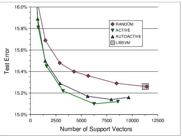
Figure 12 relates error rates and numbers of support vectors. TheRANDOM LASVMalgorithm
num-Figure 12: Comparing example selection criteria on the Adult data set. Test error as a function of the number of support vectors.
ber of support vectors of theLIBSVMsolution. Both theACTIVEandAUTOACTIVEcriteria yield
kernel classifiers with the same accuracy and much less support vectors. For instance, the
AUTOAC-TIVE LASVMalgorithm reaches the accuracy of theLIBSVMsolution using 2500 support vectors instead of 11278. Figure 11 (right plot) shows that this result is achieved after 150 seconds only.
This is about one fifteenth of the time needed to perform a fullRANDOM LASVMepoch.2
Both theACTIVE LASVMandAUTOACTIVE LASVMalgorithms exceed theLIBSVMaccuracy
after a few iterations only. This is surprising because these algorithms only use the training labels
of the few selected examples. They both outperform theLIBSVM solution by using only a small
subset of the available training labels.
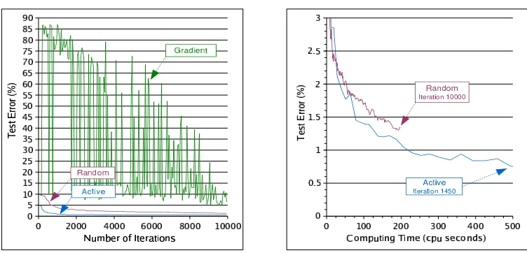
MNIST Data Set The comparatively clean MNIST data set provides a good opportunity to verify the behavior of the various example selection criteria on a problem with a much lower error rate.
Figure 13 compares the performance of theRANDOM,GRADIENTandACTIVEcriteria on the
classification of digit “8” versus all other digits. The curves are averaged on 5 runs using different
random seeds. All runs use the standard MNIST training and test sets. Both theGRADIENTand
ACTIVE criteria perform similarly on this relatively clean data set. They require about as much
computing time asRANDOMexample selection to achieve a similar test error.
Adding ten percent label noise on the MNIST training data provides additional insight regarding the relation between noisy data and example selection criteria. Label noise was not applied to the testing set because the resulting measurement can be readily compared to test errors achieved by training SVMs without label noise. The expected test errors under similar label noise conditions can be derived from the test errors measured without label noise. Figure 14 shows the test errors
achieved when 10% label noise is added to the training examples. TheGRADIENT selection
Figure 13: Comparing example selection criteria on the MNIST data set, recognizing digit “8” against all other classes. Gradient selection and Active selection perform similarly on this relatively noiseless task.
Figure 15: Comparing example selection criteria on the MNIST data set. Active example selection is insensitive to the artificial label noise.
terion causes a very chaotic convergence because it keeps selecting mislabelled training examples. TheACTIVEselection criterion is obviously undisturbed by the label noise.
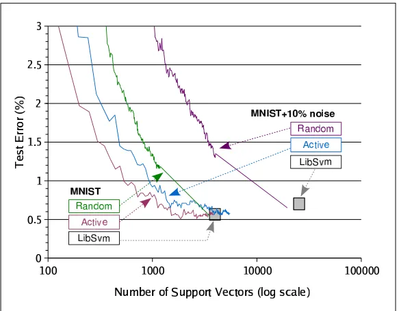
Figure 15 summarizes error rates and number of support vectors for all noise conditions. In the
presence of label noise on the training data, LIBSVMyields a slightly higher test error rate, and a
much larger number of support vectors. TheRANDOM LASVMalgorithm replicates the LIBSVM
results after one epoch. Regardless of the noise conditions, theACTIVE LASVMalgorithm reaches
the accuracy and the number of support vectors of theLIBSVMsolution obtained with clean training
data. Although we have not been able to observe it on this data set, we expect that, after a very long
time, the ACTIVE curve for the noisy training set converges to the accuracy and the number of
support vectors achieved of theLIBSVMsolution obtained for the noisy training data.
4.5 Online SVMs for Active Learning
TheACTIVE LASVMalgorithm implements two dramatic speedups with respect to existing active learning algorithms such as (Campbell et al., 2000; Schohn and Cohn, 2000; Tong and Koller, 2000). First it chooses a query by sampling a small number of random examples instead of scanning all
unlabelled examples. Second, it uses a single LASVM iteration after each query instead of fully
retraining the SVM.
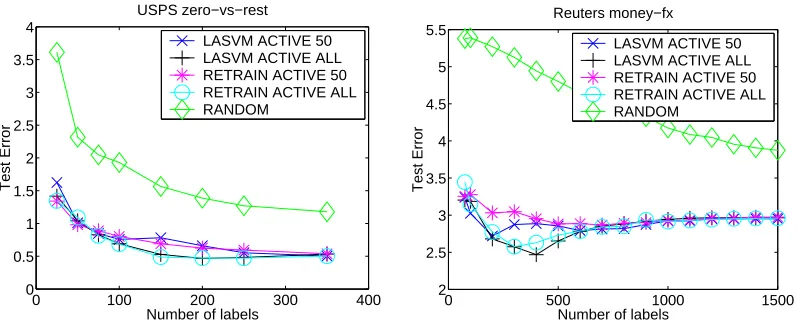
Figure 16 reports experiments performed on the Reuters and USPS data sets presented in table
7. TheRETRAIN ACTIVE 50andRETRAIN ACTIVE ALLselect a query from 50 or all unlabeled
examples respectively, and then retrain the SVM. The SVM solver was initialized with the solution
from the previous iteration. TheLASVM ACTIVE 50andLASVM ACTIVE ALLdo not retrain the
0 100 200 300 400 0 0.5 1 1.5 2 2.5 3 3.5 4
Number of labels
Test Error
USPS zero−vs−rest
LASVM ACTIVE 50 LASVM ACTIVE ALL RETRAIN ACTIVE 50 RETRAIN ACTIVE ALL RANDOM
0 500 1000 1500
2 2.5 3 3.5 4 4.5 5 5.5
Number of labels
Test Error
Reuters money−fx
LASVM ACTIVE 50 LASVM ACTIVE ALL RETRAIN ACTIVE 50 RETRAIN ACTIVE ALL RANDOM
Figure 16: Comparing active learning methods on the USPS and Reuters data sets. Results are
averaged on 10 random choices of training and test sets. UsingLASVMiterations instead
ofretraining causes no loss of accuracy. Sampling M=50 examples instead of searching all examples only causes a minor loss of accuracy when the number of labeled examples is very small.
All the active learning methods performed approximately the same, and were superior to
ran-dom selection. UsingLASVMiterations instead of retraining causes no loss of accuracy. Sampling
M=50 examples instead of searching all examples only causes a minor loss of accuracy when the
number of labeled examples is very small. Yet the speedups are very significant: for 500 queried
labels on the Reuters data set, theRETRAIN ACTIVE ALL,LASVM ACTIVE ALL, andLASVM
AC-TIVE 50algorithms took 917 seconds, 99 seconds, and 9.6 seconds respectively.
5. Discussion
This work started because we observed that the data set sizes are quickly outgrowing the computing power of our calculators. One possible avenue consists of harnessing the computing power of multiple computers (Graf et al., 2005). Instead we propose learning algorithms that remain closely related to SVMs but require less computational resources. This section discusses their practical and theoretical implications.
5.1 Practical Significance
When we have access to an abundant source of training examples, the simple way to reduce the complexity of a learning algorithm consists of picking a random subset of training examples and running a regular training algorithm on this subset. Unfortunately this approach renounces the more accurate models that the large training set could afford. This is why we say, by reference to statistical efficiency, that an efficient learning algorithm should at least pay a brief look at every training example.
The onlineLASVMalgorithm is very attractive because it matches the performance of a SVM
faster than a SVM (figure 2) and using much less memory than a SVM (figure 6). This is very im-portant in practice because modern data storage devices are most effective when the data is accessed sequentially.
Active Selection of the LASVM training examples brings two additional benefits for practical
applications. It achieves equivalent performances with significantly less support vectors, further reducing the required time and memory. It also offers an obvious opportunity to parallelize the search for informative examples.
5.2 Informative Examples and Support Vectors
By suggesting that all examples should not be given equal attention, we first state that all training examples are not equally informative. This question has been asked and answered in various con-texts (Fedorov, 1972; Cohn et al., 1990; MacKay, 1992). We also ask whether these differences can be exploited to reduce the computational requirements of learning algorithms. Our work answers this question by proposing algorithms that exploit these differences and achieve very competitive performances.
Kernel classifiers in general distinguish the few training examples named support vectors. Ker-nel classifier algorithms usually maintain an active set of potential support vectors and work by iterations. Their computing requirements are readily associated with the training examples that be-long to the active set. Adding a training example to the active set increases the computing time associated with each subsequent iteration because they will require additional kernel computations involving this new support vector. Removing a training example from the active set reduces the cost of each subsequent iteration. However it is unclear how such changes affect the number of subsequent iterations needed to reach a satisfactory performance level.
Online kernel algorithms, such as the kernel perceptrons usually produce different classifiers when given different sequences of training examples. Section 3 proposes an online kernel algorithm that converges to the SVM solution after many epochs. The final set of support vectors is intrin-sically defined by the SVM QP problem, regardless of the path followed by the online learning process. Intrinsic support vectors provide a benchmark to evaluate the impact of changes in the ac-tive set of current support vectors. Augmenting the acac-tive set with an example that is not an intrinsic support vector moderately increases the cost of each iteration without clear benefits. Discarding an example that is an intrinsic support vector incurs a much higher cost. Additional iterations will be necessary to recapture the missing support vector. Empirical evidence is presented in Section 3.5.
Nothing guarantees however that the most informative examples are the support vectors of the SVM solution. Bakır et al. (2005) interpret Steinwart’s theorem (Steinwart, 2004) as an indication that the number of SVM support vectors is asymptotically driven by the examples located on the wrong side of the optimal decision boundary. Although such outliers might play a useful role in the construction of a decision boundary, it seems unwise to give them the bulk of the available
com-puting time. Section 4 adds explicit example selection criteria toLASVM. The Gradient Selection
5.3 Theoretical Questions
The appendix provides a comprehensive analysis of the convergence of the algorithms discussed in this contribution. Such convergence results are useful but limited in scope. This section underlines some aspects of this work that would vastly benefit from a deeper theoretical understanding.
• Empirical evidence suggests that a single epoch of theLASVMalgorithm yields
misclassifi-cation rates comparable with a SVM. We also know thatLASVMexactly reaches the SVM
solution after a sufficient number of epochs. Can we theoretically estimate the expected dif-ference between the first epoch test error and the many epoch test error? Such results exist for well designed online learning algorithms based on stochastic gradient descent (Murata and Amari, 1999; Bottou and LeCun, 2005). Unfortunately these results do not directly apply to kernel classifiers. A better understanding would certainly suggest improved algorithms.
• Test error rates are sometimes improved by active example selection. In fact this effect has
already been observed in the active learning setups (Schohn and Cohn, 2000). This small improvement is difficult to exploit in practice because it requires very sensitive early stopping criteria. Yet it demands an explanation because it seems that one gets a better performance by using less information. There are three potential explanations: (i) active selection works well on unbalanced data sets because it tends to pick equal number of examples of each class (Schohn and Cohn, 2000), (ii) active selection improves the SVM loss function because it discards distant outliers, (iii) active selection leads to more sparse kernel expansions with better generalization abilities (Cesa-Bianchi et al., 2005). These three explanations may be related.
• We know that the number of SVM support vectors scales linearly with the number of examples
(Steinwart, 2004). Empirical evidence suggests that active example selection yields transitory kernel classifiers that achieve low error rates with much less support vectors. What is the scaling law for this new number of support vectors?
• What is the minimal computational cost for learning n independent examples and achieving
“optimal” test error rates? The answer depends of course of how we define these “optimal” test error rates. This cost intuitively scales at least linearly with n because one must pay a look at each example to fully exploit them. The present work suggest that this cost might be smaller than n times the reduced number of support vectors achievable with the active learning technique. This range is consistent with previous work showing that stochastic gra-dient algorithms can train a fixed capacity model in linear time (Bottou and LeCun, 2005). Learning seems to be much easier than computing the optimum of the empirical loss.
5.4 Future Directions
Progress can also be achieved along less arduous directions.
• Section 3.5 suggests that better convergence speed could be attained by cleverly modulating
the number of calls toREPROCESSduring the online iterations. Simple heuristics might go a
• Section 4.3 suggests a heuristic to adapt the sampling size for the randomized search of
in-formative training examples. ThisAUTOACTIVEheuristic performs very well and deserves
further investigation.
• Sometimes one can generate a very large number of training examples by exploiting known
invariances. Active example selection can drive the generation of examples. This idea was suggested in (Loosli et al., 2004) for the SimpleSVM.
6. Conclusion
This work explores various ways to speedup kernel classifiers by asking which examples deserve more computing time. We have proposed a novel online algorithm that converges to the SVM
solu-tion.LASVMreliably reaches competitive accuracies after performing a single pass over the training
examples, outspeeding state-of-the-art SVM solvers. We have then shown how active example se-lection can yield faster training, higher accuracies and simpler models using only a fraction of the training examples labels.
Acknowledgments
Part of this work was funded by NSF grant CCR-0325463. We also thank Eric Cosatto, Hans-Peter Graf, C. Lee Giles and Vladimir Vapnik for their advice and support, Ronan Collobert and Chih-Jen Lin for thoroughly checking the mathematical appendix, and Sathiya Keerthi for pointing out reference (Takahashi and Nishi, 2003).
Appendix A. Convex Programming with Witness Families
This appendix presents theoretical elements about convex programming algorithms that rely on successive direction searches. Results are presented for the case where directions are selected from a well chosen finite pool, like SMO (Platt, 1999), and for the stochastic algorithms, like the online and active SVM discussed in the body of this contribution.
Consider a compact convex subset
F
ofRnand a concave function f defined onF
. We assumethat f is twice differentiable with continuous derivatives. This appendix discusses the maximization of function f over set F:
max
x∈F f(x). (14)
This discussion starts with some results about feasible directions. Then it introduces the notion of witness family of directions which leads to a more compact characterization of the optimum. Finally it presents maximization algorithms and establishes their convergence to approximate solu-tions
A.1 Feasible Directions
Notations Given a point x∈