Learning Latent Variable Models by Pairwise Cluster
Comparison: Part I
−
Theory and Overview
Nuaman Asbeh [email protected]
Department of Industrial Engineering and Management Ben-Gurion University of the Negev
Beer Sheva, 84105, Israel
Boaz Lerner [email protected]
Department of Industrial Engineering and Management Ben-Gurion University of the Negev
Beer Sheva, 84105, Israel
Editors:Isabelle Guyon and Alexander Statnikov
Abstract
Identification of latent variables that govern a problem and the relationships among them, given measurements in the observed world, are important for causal discovery. This iden-tification can be accomplished by analyzing the constraints imposed by the latents in the measurements. We introduce the concept ofpairwise cluster comparison(PCC) to identify causal relationships from clusters of data points and provide a two-stage algorithm called learning PCC(LPCC) that learns a latent variable model (LVM) using PCC. First, LPCC learns exogenous latents and latent colliders, as well as their observed descendants, by using pairwise comparisons between data clusters in the measurement space that may explain latent causes. Since in this first stage LPCC cannot distinguish endogenous la-tent non-colliders from their exogenous ancestors, a second stage is needed to extract the former, with their observed children, from the latter. If the true graph has no serial connections, LPCC returns the true graph, and if the true graph has a serial connection, LPCC returns a pattern of the true graph. LPCC’s most important advantage is that it is not limited to linear or latent-tree models and makes only mild assumptions about the distribution. The paper is divided in two parts: Part I (this paper) provides the necessary preliminaries, theoretical foundation to PCC, and an overview of LPCC; Part II formally introduces the LPCC algorithm and experimentally evaluates its merit in different syn-thetic and real domains. The code for the LPCC algorithm and data sets used in the experiments reported in Part II are availableonline.
Keywords: causal discovery, clustering, learning latent variable model, multiple indica-tor model, pure measurement model
1. Introduction
play a key role in scientific theories and models, and yet such entities are latent (Klee, 1997).
Sometimes, latent variables correspond to aspects of physical reality that could, in principle, be measured but may not be for practical reasons, for example, “quarks”. In this situation, the term hidden variables is commonly used, reflecting the fact that the variables are “really there”, but hidden. On the other hand, latent variables may not be physically real but instead correspond to abstract concepts such as “psychological stress” or “mental states”. The terms hypothetical variables or hypothetical constructs may be used in these situations.
Latent variable models (LVMs) represent latent variables and the causal relationships among them to explain observed variables that have been measured in the domain. These models are common and essential in diverse areas, such as in economics, social sciences, psychology, natural language processing, and machine learning. Thus, they have recently become the focus of an increasing number of studies. LVMs reduce dimensionality by aggregating (many) observed variables into a few latent variables, each of which represents a “concept” explaining some aspects of the domain that can be interpreted from the data. Latent variable modeling is a century-old enterprise in statistics. It originated with the work of Spearman (1904), who developed factor analytic models for continuous variables in the context of intelligence testing.
Learning an LVM exploits values of the measured variables as manifested in the data to make an inference about the causal relationships among the latent variables and to pre-dict the value of these variables. Statistical methods for learning an LVM, such as factor analysis, are most commonly used to reveal the existence and influence of latent variables. Although these methods effectively reduce dimensionality and may fit the data reasonably well, the resulting models might not have any correspondence to real causal mechanisms (Silva et al., 2006). On the other hand, the focus of learning Bayesian networks (BNs) is on causal relations among observed variables, whereas the detection of latent variables and the interrelations among themselves and with the observed variables has received little at-tention. Learning an LVM using Inductive Causation* (IC*) (Pearl, 2000; Pearl and Verma, 1991) and Fast Causal Inference (FCI) (Spirtes et al., 2000) returns partial ancestral graphs, which indicate for each link whether it is a (potential) manifestation of a hidden common cause for the two linked variables. The structural EM algorithm (Friedman, 1998) learns a structure using a fixed set of previously given latents. By searching for “structural sig-natures” of latents, the FindHidden algorithm (Elidan et al., 2000) detects substructures that suggest the presence of latents in the form of dense subnetworks. Elidan and Fried-man (2001) give a fast algorithm for determining the cardinality – the number of possible states – of latent variables introduced this way. However, Silva et al. (2006) suspected that FindHidden cannot always find a pure measurement sub-model,1which is a flaw in causal analysis. Also, the recovery of latent trees of binary and Gaussian variables has been sug-gested (Pearl, 2000). Hierarchical latent class (HLC) models, which are rooted trees where the leaf nodes are observed while all other nodes are latent, were proposed for the clus-tering of categorical data (Zhang, 2004). Two greedy algorithms are suggested (Harmeling
and Williams, 2011) to expedite learning of both the structure of a binary HLC and the cardinalities of the latents. The BIN-G algorithm determines both the structure of the tree and the cardinality of the latent variables in a bottom-up fashion. The BIN-A algorithm first determines the tree structure using agglomerative hierarchical clustering and then determines the cardinality of the latent variables in the same manner as the BIN-G algo-rithm. Latent-tree models are also used to speed approximate inference in BN, trading the approximation accuracy with inferential complexity (Wang et al., 2008).
Models in which multiple latents may have multiple indicators (observed children), also known as multiple indicator models (MIMs) (Bartholomew et al., 2002; Spirtes, 2013), are a very important subclass of structural equation models (SEM), which are widely used, together with BNs, in applied and social sciences to analyze causal relations (Pearl, 2000; Shimizu et al., 2011). For these models, and others that are not tree-constrained, most of the mentioned algorithms may lead to unsatisfactory results. This is one of the most difficult problems in machine learning and statistics since, in general, a joint distribution can be generated by an infinite number of different LVMs. However, an algorithm that fills the gap between learning latent-tree models and learning MIMs is BuildPureClusters (BPC; Silva et al., 2006). BPC searches for the set (an equivalence class) of MIMs that best matches the set of vanishing tetrad differences (Scheines et al., 1995), but is limited to linear models (Spirtes, 2013).
In this study, we make another attempt in this direction and target the goal of Silva et al. (2006), but concentrate on the discrete case, rather than on the continuous case dealt with BPC. Towards this mission, we borrow ideas and principles of clustering and unsu-pervised learning. Interestingly, the same difficulty in learning MIMs is also faced in the domain of unsupervised learning that confronts similar questions such as: (1) How many clusters are there in the observed data? and (2) Which classes do the clusters really repre-sent? Due to this similarity, our study suggests linking the two domains – learning a causal graphical model with latent variables and clustering analysis. We propose a concept and an algorithm that combine learning causal graphical models with clustering. According to thepairwise cluster comparison(PCC) concept, we compare pairwise clusters of data points representing instantiations of the observed variables to identify those pairs of clusters that exhibit major changes in the observed variables due to changes in their ancestor latent variables. Changes in a latent variable that are manifested in changes in the observed vari-ables reveal this latent variable and its causal paths of influence in the domain. Using the learning PCC(LPCC) algorithm, we learn an LVM. We identify PCCs and use them to learn latent variables – exogenous and endogenous (the latter may be either colliders or non-colliders) – and their causal interrelationships as well as their children (latent variables and observed variables) and causal paths from latent variables to observed variables.
Part I:
• Section 2: Preliminaries to LVM learning describes the assumptions of our ap-proach and basic definitions of essential concepts of graphical models and SEM;
• Section 3: Preliminaries to LPCC formalizes our ideas and builds the theoretical basis for LPCC;
• Section 4: Overview of LPCC starts with an illustrative example and a broad de-scription of the LPCC algorithm and then describes each step of LPCC in detail;
• Section 5: Discussion and future researchsummarizes and discusses the contribu-tion of LPCC and suggests several new avenues of research;
• Appendix Aprovides proofs to all propositions, lemmas, and theorems for which the proof is either too detailed, lengthy, or impedes the flow of reading. All other proofs are given in the body of the paper;
• Appendix Bsets a method to calculate a threshold in support of Section 4.4; and
• Appendix Csupplies a detailed list of assumptions LPCC makes and the meaning of their violation.
Part II:
• Section 2: The LPCC algorithmintroduces and formally describes a two-stage algo-rithm that implements the PCC concept;
• Section 3: LPCC evaluationevaluates LPCC, in comparison to state-of-the-art algo-rithms, using simulated and real-world data sets;
• Section 4: Related works compares LPCC to state-of-the-art LVM learning algo-rithms;
• Section 5: Discussionsummarizes the theoretical advantages (from Part I) and the practical benefits (from this part) of using LPCC;
• Appendix Abrings assumptions, definitions, propositions, and theorems from Part I that are essential to Part II;
• Appendix Bsupplies additional results for the experiments with the simulated data sets; and
2. Preliminaries to LVM learning
The goal of our study is to reconstruct an LVM from i.i.d. data sampled from the observed variables in an unknown model. To accomplish this, we propose learning from pairwise cluster comparison using LPCC. First, we present the assumptions that LPCC makes and the constraints it applies on LVM and compare them to those required by other state-of-the-art methods.
Assumption 1 The underlying model is a Bayesian network, BN=<G,Θ>, encoding a discrete joint probability distribution P for a set of random variables V=L∪O, where G=<V,E> is a directed acyclic graph (DAG) whose nodesVcorrespond to latentsLand observed variablesO, andE is the set of edges between nodes in G. Θ is the set of parameters, i.e., the conditional probabilities of variables inVgiven their parents.
Assumption 2 No observed variable inOis an ancestor of any latent variable inL.This prop-erty is called themeasurement assumption(Spirtes et al., 2000).
Before we present additional assumptions about the learned LVM, we need Definitions 1–4 (following Silva et al., 2006), which are specific to LVM:
Definition 1 A model satisfying Assumptions 1 and 2 is a latent variable model.
Definition 2 Given an LVMGwith a variable setV, the subgraph containing all variables in
Vand all and only those edges directed into variables inOis called the measurement model of
G.
Definition 3 Given an LVMG, the subgraph containing all and onlyG’s latent nodes and their respective edges is called the structural model ofG.
When each model variable is a linear function of its parents in the graph plus an ad-ditive error term of positive finite variance, the latent variable model is linear; this is also known as SEM. Great interest has been shown in linear LVMs and their applications in social science, econometrics, and psychometrics (Bollen, 1989), as well as in their learning (Silva et al., 2006). The motivation to use linear models usually comes from social and related sciences. For example,2 researchers give subjects a questionnaire with questions like: “On a scale of 1 to 5, how much do you agree with the statement: ‘I feel sad every day’.” The answer is measured by an observed variable, and the linearity of the influence of an unknown cause (say depression in this case) on the answer (value) to the question is assumed. By using other questions, which researchers assume also measure depression, they expect to discover a latent depression variable that is a parent of several observed variables (each measuring a question), together indicating depression. It is common to re-quire several questions/observed variables for the identification of each latent variable and to consider the information revealed through only a single question as noise, which cannot guarantee the identification of the latent. Researchers expect that other questions will be clustered by another latent variable that measures another aspect in the domain, and thus
questions of one cluster will be independent of questions of another cluster conditioned on the latent variables. They also attribute unconditional independence that is detected between observed variables of different clusters to errors in the learning algorithm.
Adding the linearity assumption to Assumptions 1 and 2 allows for the transforma-tion of Definitransforma-tion 1 into that of a linear LVM. Since assuming linearity means linearity is assumed in the measurement model, a key to learning a linear LVM is learning the mea-surement model and only then the structural model. In learning the meamea-surement model of MIM, the linearity assumption entails constraints on the covariance matrix of the ob-served variables and thereby eliminates learning co-variants (dependences) between pairs of observed variables that “should” not be connected in the learned model (Silva et al., 2006; Spirtes, 2013). If, however, the linearity assumption does not hold, the algorithms suggested in Silva et al. (2006) may not find a model and would output a “can’t tell” an-swer, which is, nevertheless, a better result than learning an incorrect model.
In this study, we dispense with the linearity assumption and apply the above con-cepts to learn not necessarily linear MIMs or latent-tree models. Our suggested algorithm, LPCC, is not limited by the linearity assumption and learns a model as long as it is MIM. In addition, we are interested in discrete LVMs.
Another important definition we need is:
Definition 4 A pure measurement model is a measurement model in which each observed vari-able has only one latent parent and no observed parent.
Assumption 3 The measurement model ofGis pure.
As a principled way of testing conditional independence among latents, Silva et al. (2006) focus on MIMs, which are pure measurement models. Practically, these models have a smaller equivalence class of the latent structure than that of non-pure models and thus are easier to unambiguously learn. Consider, for example, that we are interested in learning the topic of a document (e.g., the first page in a newspaper) from anchor word (key phrase) distributions and that this document may cover several topics (e.g., politics, sports, and finance). Simplification of this topic modeling problem, following the rep-resentation of a topic using a latent variable in LVM, can be achieved by assuming and learning a pure measurement model representing a pure topic model for which each spe-cific document covers only a single topic, which is reasonable in some cases, such as a sports or financial newspaper.
LPCC does not assume that the true measurement model is linear (which is a para-metric assumption that, e.g., BPC makes), but rather assumes that the model is pure (a structural assumption). When the true causal model is pure, LPCC will identify it cor-rectly (or find its pattern that represents the equivalence class of the true graph). When it is not pure, LPCC – similarly to BPC (Silva et al., 2006) – will learn a pure sub-model of the true model using two indicators for each latent (compared to three indicators per latent that are required by BPC). Part II of this paper presents several examples of real-world problems from different domains for which LPCC learns a pure (sometimes sub-) model, never less accurately than other methods.
Assumption 4 The true modelGis MIM, in which each latent has at least two observed chil-dren and may have latent parents.
Causal structure discovery – learning the number of latent variables in the model, their interconnections and connections to the observed variables, as well as the interconnections among the observed variables – is very difficult and thus requires making some assump-tions about the problem. Particularly, MIMs, in which multiple observed variables are assumed to be affected by latent variables and perhaps by each other (Spirtes, 2013), are reasonable models but have attracted scant attention in the machine-learning community. As Silva et al. (2006) pointed out, factor analysis, principal component analysis, and re-gression analysis adapted to learning LVMs are well understood but have not been proven, under any general assumptions, to learn the true causal LVM, calling for better learning methods. By assuming that the true model manifests local influence of each latent variable on at least a small number of observed variables, Silva et al. (2006) showed that learning the complete Markov equivalence class of MIM is feasible. Similar to Silva et al. (2006), we assume that the true model is MIM; thus, this is where we place our focus on learning. Note also that based on Assumptions 3 and 4, the observed variables inGare d-separated, given the latents.
3. Preliminaries to LPCC
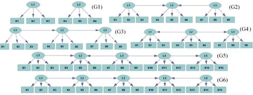
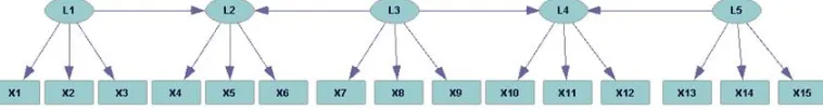
Figure 1 sketches a range of MIMs, which all exhibit pure measurement models, from ba-sic to more complex models. Compared to G1, which is a baba-sic MIM of two unconnected latents, G2 shows a structural model that is characterized by a latent collider. Note that such an LVM cannot be learned by latent-tree algorithms such as in Zhang (2004). G3 and G4 demonstrate serial and diverging structural models, respectively, that together with G2 cover the three basic structural models. G5 and G6 manifest more complex structural models comprising a latent collider and a combination of serial and diverging connections. As the structural model becomes more complicated, the learning task becomes more chal-lenging; hence, G1–G6 present a spectrum of such challenges to an LVM learning algo-rithm.3
In Section 3.1, we build the infrastructure to pairwise cluster comparison that relies on understanding the influence of the exogenous latent variables on the observed variables in the LVM. This influence is divided into major and minor effects that are introduced and explained in Section 3.2. In Section 3.3, we link this structural influence to data clustering and introduce the pairwise cluster comparison concept for learning an LVM.
3.1 The influence of exogenous latents on observed variables is fundamental to learning an LVM
We distinguish between observed (O)and latent (L)variables and between exogenous (EX) and endogenous (EN) variables. EXhave zero in-degree, are autonomous, and unaffected
Figure 1: Example LVMs that are all MIMs. Each is based on a pure measurement model and a structural model of different complexity, posing a different challenge to a learning algorithm.
by the values of the other variables (e.g., L1 in all graphs but G4 in Figure 1), whereas
EN are all non-exogenous variables in G(e.g., L2 in all graphs but G1 and G4, and X1 in all graphs in Figure 1). We identify three types of variables: (1) Exogenous latents,
EX⊂(L∩NC) [all exogenous variables are latent non-colliders (NC)]; (2) Endogenous la-tents, EL⊂(L∩EN), which are divided into latent colliders C⊂EL(e.g., L2 in G2 and G5; note that all latent colliders are endogenous) and latent non-colliders (in serial and di-verging connections)S⊂(EL∩NC)(e.g., L3 in G3, G4, and G6), thusNC= (EX∪S); and (3) Observed variables,O⊂EN, which are always endogenous and childless, that are divided into children of exogenous latentsOEX⊂O(e.g., X1 and X9 in G2), children of latent col-lidersOC⊂O(e.g., X4, X5, and X6 in G2), and children of endogenous latent non-colliders
OS⊂O(e.g., X4, X5, and X6 in G3). We denote value configurations ofEX,EN(when we do not know whether the endogenous variables are latent or observed),EL,C,NC(when we do not know whether the non-collider variables are exogenous or endogenous), S, O,
OEX,OC, andOSbyex,en,el,c,nc,s,o,oex,oc, andos, respectively.
Since the underlying model is a BN, the joint probability overV, which is represented by the BN, is factored according to the local Markov assumption forG. That is, any variable inVis independent of its non-descendants inGconditioned on its parents inG:
P(V) =Y
Vi∈V
P(Vi|Pa
wherePai are the parents ofVi. It can be factorized under our assumptions as:
P(V) =P(EX,C,S,OEX,OC,OS) =
Y
EXi∈EX
P(EXi)
Y
Cj∈C
P(Cj|Paj)
Y
St∈S
P(St|P at)
Y
OEXm∈OEX
P(OEXm|EXm)
Y
OCk∈OC
P(OCk|Ck)
Y
OSv∈OS
P(OSv|Sv) (2)
where Paj are the latent parents of the latent collider Cj, P at is the latent parent of the
latent non-collider St (in other words, Paj, P at⊂NC), Ck∈C and Sv∈Sare the latent
col-lider and latent non-colcol-lider parents of observed variablesOCkandOSv, respectively, and EXm∈EXis the exogenous latent parent of observed variableOEXm.
In this paper, we claim and demonstrate that the influence of exogenous (latent) vari-ables on observed varivari-ables is fundamental to learning an LVM and introduce LPCC that identifies and exploits this influence to learn an MIM. In this section, we prove that changes in values of the observed variables are due to changes in values of the exogenous variables and thus the identification of the former indicates the existence of the latter. To do that, we analyze the propagation of influence along paths connecting both variables, remem-bering that the paths may contain latent colliders and latent non-colliders. First, however, we should analyze paths among the latents and only then paths ending in their sinks (i.e., the observed variables). To prove that all changes in the graph, and specifically those measured in the observed variables, are the result of changes in the exogenous latent vari-ables, we will need to first provide some definitions (following Spirtes et al., 2000; Pearl, 1988, 2000) of paths and some assumptions about the possible paths between latents in the structural model.
Definition 5 A path between two nodesV1 andVn in a graph Gis a sequence of nodes{V1, ..., Vn}, such that Viand Vi+1are adjacent inG, 1≤i<n, i.e.,{Vi, Vi+1} ∈E.
Note that a unique set of edges is associated with each given path. Paths are assumed to be simple by definition; in other words, no node appears in a path more than once, and an empty path consists of a single node.
Definition 6 A collider on a path{V1, ..., Vn}is a nodeVi,1< i < n, such thatVi−1andVi+1are parents ofVi.
Definition 7 A directed pathTVnfromV1toVnin a graphGis a path between these two nodes, such that for every pair of consecutive nodes Vi and Vi+1, 1≤i<n on the path, there is an edge from Vi into Vi+1inE. V1is the source, andVn is the sink of the path. A directed path has no
colliders.
to be colliders). This shows a tradeoffbetween the structural and parametric assumptions that an algorithm for learning an LVM usually has to make; the fewer parametric assump-tions the algorithm makes, the more structural assumpassump-tions it has to make and vice versa.
Assumption 5 A latent collider does not have any latent descendants (and thus cannot be a parent of another latent collider).
To distinguish between latent colliders and latent non-colliders, their observed chil-dren, and their connectivity patterns to their exogenous variables, we use Lemma 1. La-tent colliders and their observed children are connected to several exogenous variables via several directed paths, whereas latent non-colliders and their observed children are con-nected only to a single exogenous variable via a single directed path. Use of these different connectivity patterns – from exogenous latents through endogenous latents (both colliders and non-colliders) to observed variables – simplifies (2) and the analysis of the influence of latents on observed variables.
Lemma 1
1. Each latent non-colliderN Ct has only one exogenous latent ancestorEXN Ct, and there is only one directed pathTN Ct fromEXN Ct(source) toN Ct (sink). (Note that we use the notationN Ct, rather thanSt, since the lemma
ap-plies to both exogenous and endogenous latent non-colliders.)
2. Each latent collider Cj is connected to a set of exogenous latent ancestors
EXCj via a set of directed pathsTCj fromEXCj (sources) toCj (sink).
Lemma 1 allows us to separate the influence of all exogenous variables to separate paths of influence, each from exogenous to observed variables. Proposition 1 quantifies the propa-gation of this influence along the paths through the joint probability distribution.
Proposition 1 The joint probability overVdue to value assignmentexto exogenous setEXis determined only by this assignment and the BN conditional probabilities.
Proof The first product in (2) for assignmentexis ofex’s priors. In the other five prod-ucts, the probabilities are of endogenous latents or observed variables conditioned on their parents, which, based on Lemma 1, are either on the directed paths from EXto the la-tents/observed variables or exogenous themselves. Either way, any assignment of endoge-nous latents or observed variables is a result of the assignmentexto EXthat is mediated to the endogenous latents/observed variables by the BN probabilities:
P(V|EX=ex) =P(EX,C,S,OEX,OC,OS|EX=ex) =
Y
EXi∈EX
P(EXi=exi)
Y
Cj∈C
P(Cj=cj|Paj=pa exCj
j )
Y
St∈S
P(St=nct|P at=pa exSt
t ) (3)
Y
OEXm∈OEX
P(OEXm=oexm|EXm=exm)
Y
OCk∈OC
P(OCk=ock|Ck=c exCk
k )
Y
OSv∈OS
P(OSv=osv|Sv=s exSv v )
• exiandexmare the values ofEXiandEXm(the latter is the parent of themth observed
child of the exogenous latents), respectively, in the assignmentextoEX;
• paexj Cj is the configuration ofCj’s parents due to configurationexCj ofCj’s exogenous ancestors inex;
• paext St is the value ofSt’s parent due to the valueexSt ofSt’s exogenous ancestor inex;
• cexk Ck is the value ofOCk’s collider parent due to the configurationexCk ofCk’s exoge-nous ancestors inex; and
• svexSv is the value ofOSv’s non-collider parent due to the valueexSv ofSv’s exogenous ancestor inex.
Proposition 1 along with Lemma 1 are a key in our analysis because they show paths of hierarchical influence of latents on observed variables – from exogenous latents through endogenous latents (both colliders and non-colliders) to observed variables. Recognition and use of these paths of influence guides LPCC in learning LVMs.
To formalize our ideas, we introduce several concepts in Section 3.2. First, we define local influence on a singleENof its direct parents. Second, we use local influences and the BN Markov property to generalize the influence ofEXonEN. Third, exploiting the connec-tivity between the exogenous ancestors and their endogenous descendants, as described by Lemma 1, we focus on the influence of a specific (partial) set of exogenous variables on the values of their endogenous descendants. Analysis of the influence of all configurationsexs on all ens and that of the configurations of specific exogenous ancestors in theseexs on their endogenous descendants enable learning the structure and parameters of the model and causal discovery. Finally, in Section 3.3, we show how these concepts can be exploited to learn an LVM from data clustering.
3.2 Major and minor effects and values
So far, we have analyzed the structural influences (path of hierarchies) of the latents on the observed variables. In this section, we complement this analysis with the parametric influences, which we divide into major and minor effects.
Definition 8 A local effect on an endogenous variable EN is the influence of a configuration of EN’s direct latent parents on any of EN’s values.
1. A major local effect is the largest local effect onENi, and it is identified by the maximal conditional probability of a specific valueeni ofENi given a configurationpai ofENi’s
latent parentsPai, which isMAEENi(pai) =maxen
0
iP(ENi=en 0
i|Pai=pai).
2. A minor local effect is any non-major local effect onENi, and it is identified by a
3. A major local value is theenicorresponding toMAEENi(pai), i.e., the most probable value ofENidue topai,MAVENi(pai) =argmaxen0
iP(ENi=en 0
i|Pai=pai).
4. A minor local value is aneni corresponding to a minor local effect, andMIV SENi(pai)is the set of all minor values that correspond toMIESENi(pai).
WhenENi is an observed variable or an endogenous latent non-collider, and thus
has only a single parentP ai, the configurationpaiis actually the valuepaiofP ai.
So far, we have listed our assumptions about the structure of the model. Following is a parametric assumption:
Assumption 6 For every endogenous variableENi inGand every configurationpa0i ofENi’s
parentsPai, there exists a certain valueen0iofENi, such thatP(ENi=en0i|Pa
i=pa
0
i)> P(ENi= en00i|Pai = pa0
i) for every other value en
00
i of ENi. This assumption is related to the most
probable explanation of a hypothesis given the data (Pearl, 1988).
Note that in the case that Assumption 6 is violated, in other words, if more than one value of ENi gets the maximum probability value given a configuration of parents, LPCC still learns a model because the implementation will randomly choose a value that maximizes the probability as the most probable. However, the correctness of the algorithm is guaran-teed only if all assumptions are valid; in other words, given the assumptions are valid, all causal claims made by the output graph are correct.
Proposition 2 The major local value MAVENipa0i of an endogenous variable ENi given a certain configuration of its parentspa0iis also certain.
Proof Assumption 6 guarantees that given a certain configurationpa0i ofPai, there exists
a certain valueen0iofENi, such thatP(ENi=en0i|Pa
i=pa
0
i)> P(ENi=en
00
i|Pai=pa
0
i) for
ev-ery other valueen00i ofENi. From the definition of a major local value,MAVENi
pa0i=en0i.
We need one additional assumption about the model parameters that reflects parent-child influence in the causal model. Specifically, to identify parent-parent-child relations, LPCC needs for each observed variable or endogenous latent non-collider to get different MAVs for different values of their latent parent. Similarly, LPCC needs a collider to get different values for each of its parents in at least two parent configurations in which this parent changes, whereas the other parents do not.
Assumption 7 First, for everyENi that is an observed variable or an endogenous latent non-collider and for every two valuespa0i andpa00i ofP ai,MAVENi
pa0i,MAVENi
pa0i. Second, for every Cj that is a latent collider and for every P aj ∈Pa
j, there are at least two
configu-rations pa0j andpa00j of P aj in which only the value of P aj is different and MAVCj
pa0j , MAVCj
By aggregation over all local influences, we can now generalize these concepts through the BN parameters and Markov property from local influences on specific endogenous variables to influence on all endogenous variables in the graph.
Definition 9 An effect onEN is the influence of a configuration ex ofEXon EN. The effect is measured by a value configurationenofENdue toex. A major effect (MAE) is the largest effect ofex onENand a minor effect (MIE) is any non-MAE effect ofexonEN. Also, a major value configuration (MAV) is the configurationenofENcorresponding to MAE (i.e., the most probableendue toex), and a minor value configuration is a configurationencorresponding to any MIE.
[Note the difference between a major effect, MAE, and a major local effect,MAEENi, and between a major value configuration, MAV, and a major local value,MAVENi (and simi-larly for the “minors”).]
Based on the proof of Proposition 1, we can quantify the effect ofexonEN. For exam-ple, a major effect ofexon ENcan be factorized according to the product of major local effects onEN(weighted by the product of priors,P(EXi=exi)):
MAE(ex) = Y
EXi∈EX
P(EXi=exi)Y
Cj∈C
MAECj(paexj Cj)Y
St∈S
MAESt(paexSt
t )
Y
OEXm∈OEX
MAEOEXm(exm)
Y
OCk∈OC
MAEOCk(c
exCk
k )
Y
OSv∈OS
MAEOSv(s
exSv v ) =
Y
EXi∈EX
P(EXi=exi)Y
Cj∈C
maxc0
jP(Cj =c 0
j|Paj=pa exCj
j )
Y
St∈S
maxs0
tP(St=s 0
t|P at=pa exSt t )
Y
OEXm∈OEX
maxoex0
mP(OEXm=oex 0
m|EXm=exm)
Y
OCk∈OC
maxoc0
kP(OCk=oc 0
k|Ck=c exCk
k )
Y
OSv∈OS
maxos0
vP(OSv=os 0
v|Sv=s exSv
v ). (4)
A configurationenofENin which each variable inENtakes on the major local value is major or a MAV. Any effect in which at least one EN takes on a minor local effect is minor, and any configuration in which at least one EN takes on a minor local value is minor. We denote the set of all minor effects forexwithMIES(ex) (with correspondence toMIESENi) and the set of all minor configurations withMIV S(ex) (with correspondence toMIV SENi).
Definition 10 A partial effect on a subset of endogenous variablesEN0⊆ENis the influence of a configurationex0ofEN0’s exogenous ancestorsEX0⊆EXonEN0. We define a partial major effect MAEEN0
ex0as the largest partial effect ofex0onEN0 and a partial minor effectMIEEN0
ex0
as any non-MAEEN0
ex0 partial effect of ex0 on EN0. A partial major value configuration
MAVEN0
ex0is theen0ofEN0corresponding toMAEEN0
ex0; in other words, the most prob-able en0 due to ex0, and a partial minor value configuration is an en0 corresponding to any
MIEEN0
ex0.
We are interested in representing the influence of exogenous variables on their ob-served descendants and all the variables in the directed paths connecting them. To do this, we separately analyze the (partial) effect of each exogenous variable on each observed variable for which the exogenous is its ancestor and all the latent variables along the path connecting these two. We distinguish between two cases (both are represented in Lemma 1): (1) Observed descendants inOEXandOSthat are, respectively, children of exogenous latents and children of latent non-colliders that are linked to their exogenous ancestors, each via a single directed path; and (2) Observed descendants inOCthat are children of latent colliders and linked to their exogenous ancestors via a set of directed paths through their latent collider parents. Thus, we are interested in:
1. The partial effect of a value of exogenous ancestor EXN Cv to non-collider N Cv on any configuration of the set of variables{T SN C
v\EXN Cv, ON Cv}, whereON Cv is an observed child of latent non-colliderN Cv, and T SN Cv is the set of variables in the directed path (recall Definition 7)TN Cv fromEXN Cv toN Cv. The corresponding
MAE{T S
N Cv\EXN Cv,ON Cv}
exN Cv
and MAV{T S
N Cv\EXN Cv,ON Cv}
exN Cv
are partial ma-jor effect and partial major value configuration, respectively. For example, we may be interested in the partial effect of a value ofEXN Cv =EXL5= L3 in G5 (Figure 1) on {T SN C
v\EXN Cv, ON Cv}= {T SL5\L3,X13}={L4, L5, X13}. Note that we use here the notationN Cv since we are interested in both exogenous and endogenous latent non-colliders. When we are interested in the partial effect on an observed variable inOEX, its exogenous ancestor (which is also its direct parent) is also the latent non-collider,N Cv, and the effect is not measured on any other variable but this observed variable. This isCase 1, which is analyzed below;
2. The partial effect of a configuration of exogenous variablesEXCk to colliderCkon any configuration of the set of variables {TSC
k\EXCk, OCk}, where OCk is an observed child of latent collider Ck, 4 and TSCk is the set of variables in the set of directed pathsTCk fromEXCk toCk. The correspondingMAE{TSCk\EXCk,OCk}
exCk
and
MAV{TS
Ck\EXCk,OCk}
exCk
are partial major effect and partial major value config-uration, respectively. For example, we may be interested in the partial effect of a configuration of EXCk =EXL4 ={L1,L5} in G6 (Figure 1) on {TSCk\EXCk, OCk}= {{{L1,L2,L3,L4}\{L1},{L5}\{L5}},X11}={L2,L3,L4,X11}. This isCase 2, which is ana-lyzed below.
4Throughout the paper, we use a child index also for its parent, e.g.,OC
Following, we provide detailed descriptions for these partial effects and partial val-ues for observed children of latent non-colliders (Case 1) and observed children of latent colliders (Case 2) and formalize their properties in Propositions 3–7 to set the stage for Lemma 2.
Case 1: Observed children of latent non-colliders
If the latent non-colliderN Cv is exogenous,N Cv=EXv andON Cv=OEXv, then, {T SN C
v\EXN Cv, ON Cv}=OEXv. Thus, the partial effect is simply the local effect, and the partial major effect is the major local effectMAEOEXv(exv). If the latent non-colliderN Cv is endogenous, thenN Cv =Sv andON Cv=OSv. Then, all variables in {T S
Sv\EXSv, OSv} are d-separated byEXSv fromEX\EXSv. For example,{L4, L5, X13}in G5 (Figure 1) are d-separated by L3 from L2 and its children. Thus, the effect ofexon the joint probability distribution (3) can be factored to the: a) joint probability over EX=ex; b) conditional probabilities of the influenced variables along a specific directed path that ends atOSv on EXSv =exSv (note that the valueexSt for allSt∈T SSv is the same becauseEXSt=EXv is the same exogenous ancestor of all latent non-colliders on the path toSv); and c) conditional
probabilities of all the remaining variables in the graph onEX=ex:
P(V|EX=ex) =P(EX=ex)P({T SS
v\EXSv, OSv}|EXSv =exSv)
P(V\{T SS
v\EXSv, OSv}|EX=ex) (5)
in which the second factor corresponds to the partial effect ofEXSv =exSv on T SSv\EXSv (the latent non-colliders on the path fromEXSvtoSv) andSv’s observed child,OSv, and the third factor corresponds to the influence ofEX=exon all the other (latent and observed) variables in the graph. We can write the second factor describing the partial effect of the valueexSv on the values of the variablesT SSv\EX
Sv in the directed path fromEXSv toOSv (including) as:
P({T SS
v\EXSv, OSv}|EXSv =exSv) =
Y
St∈{T SSv\EXSv}
P(St=st|P at=pa exSt
t )P(OSv =osv|Sv =s exSv
v ) (6)
The partial major effect in (4) for this directed path can be written as (note again that exSt=exSv):
MAE{T S
Sv\EXSv,OSv}(exSv) =MAE{T SSv\EXSv}(exSv)·MAEOSv(s
exSv v ) =
Y
St∈{T SSv\EXSv}
MAESt(pa
exSv
t )·MAEOSv(s
exSv
v ) (7)
Proposition 3 TheMAV{T S
N Cv\EXN Cv,ON Cv}
exN Cv
corresponding to
MAE{T S
N Cv\EXN Cv,ON Cv}
exN Cvis a certain value configuration for each certain valueexN Cv.
(Note that here we use the notationN Cv rather thanSv since the proposition applies to
Proposition 4 All corresponding values inMAV{T S
N Cv\EXN Cv,ON Cv}
ex0N C
v
and
MAV{T S
N Cv\EXN Cv,ON Cv}
ex00N C
v
, for two valuesex0N C
v andex 00
N Cv ofEXN Cv, are different.
(Here also we use the notationN Cv, since the proposition applies to both exogenous and
endogenous latent non-colliders.)
So far, we have analyzed the impact of an exogenous variable on a latent non-collider by “propagating” the exogenous (source) impact along the path to the latent non-collider (sink). Propositions 3 and 4, respectively, guarantee that a certain value of the exogenous variable is responsible for a certain value of the latent non-collider and different values of the exogenous are echoed through different values of the latent non-collider. Proposition 4 is based on the correspondence between changes in values of a latent non-collider and changes in values of its parent; a correspondence that is guaranteed by Assumption 7 (first part). Propositions 3 and 4, respectively, ensure the existence and uniqueness of the value a latent non-collider gets under the influence of an exogenous ancestor; one (Proposition 3) and only one (Proposition 4) value of the latent non-collider changes with a change in the value of the exogenous. We formalize this in the following Proposition 5.
Proposition 5 EXN Cv changes values (i.e., has two values ex0N C
v and ex
00
N Cv) if and only if
N Cvchanges values in the two corresponding major value configurations: MAV{T S
N Cv\EXN Cv,ON Cv}
ex0N C
v
andMAV{T S
N Cv\EXN Cv,ON Cv}
ex00N C
v
.
Case 2: Observed children of latent colliders
In the case of an observed variableOCk that is a child of a latent colliderCk, all variables
in {TSC
k\EXCk, OCk} are d-separated by EXCk from EX\EXCk. Thus, the effect of ex on the joint probability distribution (3) can be factored (similarly to Case 1) to the: a) joint probability overEX=ex; b) conditional probabilities of the influenced variables along all directed paths that end atOCk onEXCk =exCk(note that all variables along each directed path TCk are influenced by the sameexCk); and c) conditional probabilities of all the re-maining variables in the graph onEX=ex:
P(V|EX=ex) =P(EX=ex)P({TSC
k\EXCk, OCk}|EXCk =exCk)
P(V\{TSC
k\EXCk, OCk}|EX=ex) (8)
in which the second factor corresponds to the partial effect on{TS
Ck\EXCk, OCk}of EXCk, and the third factor corresponds to the partial effect on all variables other than
{TS
Ck\EXCk, OCk}. We can decompose the second factor into a product of: a) a product
over all directed paths intoCk of a product of partial effects over all variables (excluding Ck) in such a path; b) the partial effect onCk; and c) the partial effect on its childOCk:
P({TSC
k\EXCk, OCk}|EXCk =exCk) =
Y
T SCk∈TS Ck
Y
St∈T SCk\{EXCk,Ck}
P(St=st|P at=pa exCk
t )P(Ck=ck|Pak=pa exCk
k )P(OCk=ock|Ck=c exCk k ).
This factor can be rewritten as:
P({TSC
k\EXCk, OCk}|EXCk =exCk) =
Y
T SCk∈TS Ck
P({T SC
k\EXCk, Ck}|EXCk=exCk)P(Ck=ck|Pak=pa
exCk
k )P(OCk=ock|Ck=c exCk k ).
(10)
It reflects the partial effects of a configurationexCkon the values of the variables in{TS
Ck\EXCk} and the valuesCk andOCk get, and thus the partial major effect of the second factor can
be represented as:
MAE{TS
Ck\EXCk,OCk}(exCk) =
Y
T SCk∈TS Ck
MAE{T S
Ck\EXCk,Ck}(exCk)MAECk(pa
exCk
k )MAEOCk(c
exCk k ).
(11)
Proposition 6 TheMAV{TS
Ck\EXCk,OCk}
exCk
corresponding toMAE{TS
Ck\EXCk,OCk}
exCk
is a certain value configuration for each certain value configurationexCk.
We wish to apply the same mechanism as in Case 1 to analyze the impact of more than a single exogenous ancestor on a latent collider, but here the impact is propagated toward the collider along more than a single path. To accomplish this, the following Proposition 7 analyzes the effect on a collider of each of its exogenous ancestors by considering the effect of such an exogenous on the corresponding collider’s parent (using Proposition 5, similar to Case 1 for a latent non-collider) and then the effect of this parent on the collider itself (using the second part of Assumption 7).
Proposition 7 For every exogenous ancestorEXCk ∈EXCk of a latent colliderCk, there are at least two configurationsex0C
k andex 00
Ck ofEXCk in which onlyEXCkof allEXCk changes values whenCkchanges values in the two corresponding major value configurationsMAV{TS
Ck\EXCk,OCk}
ex0C
k
andMAV{TS
Ck\EXCk,OCk}
ex00C
k
.
Lemma 2
1. A latent non-colliderN Cv and its observed childON Cv, both descendants of
an exogenous variableEXN Cv, change their values in any two major configu-rations if and only ifEXN Cv has changed its value in the corresponding two configurations ofEX.
2. A latent collider Ck and its observed childOCk, both descendants of a set of exogenous variablesEXCk, change their values in any two major configurations only if at least one of the exogenous variables inEXCk has changed its value in the corresponding two configurations ofEX.
3.3 PCC by clustering observational data
of observed variables (which is part of a configuration of the endogenous variables) and their joint probability is a result of the assignment of a configurationexto the exogenous variablesEX. Therefore, we define:
Definition 11 An observed value configuration, observed major value configuration, and ob-served minor value configuration due toexare the parts inen, MAV, and a minor value config-uration, respectively, that correspond to the observed variables.
The following two propositions formalize the relationships between the observed ma-jor value configurations and the set of possibleex.
Proposition 8 There is only a single observed major value configuration to each exogenous configurationexofEX.
Proof Based on Lemma 2, different observed major value configurations can be obtained if and only if there is more than a single exogenous configurationexofEX. Thus, an ex-ogenous configurationexcan only lead to a single observed major value configuration.
Proposition 9 There are different observed major value configurations to different exogenous configurationsexs.
Proof Assume for the sake of contradiction that two different value configurationsex1and
ex2led to the same observed major value configuration. Because the two configurations are different, there is at least one exogenous variableEX0 that has different values inex1
andex2. Since based on Assumption 4,EX0 has at least two observed children, then, based
on Assumption 7, each of these children has different values in the two observed major value configurations due to the different value ofEX0 inex1 andex2. This is contrary to
our assumption that there is only one observed major value configuration.
Due to the probabilistic nature of BN, each observed value configuration due toexmay be represented by several data points. Clustering these data points may produce several clusters for eachexand each cluster corresponds to another observed value configuration. Based on Propositions 8 and 9, one and only one of the clusters corresponds to each of the observed major value configurations, whereas the other clusters correspond to observed minor value configurations. We distinguish between these clusters using Definition 12.
Definition 12 The single cluster that corresponds to the observed major value configuration, and thus also represents the major effectMAE(ex)due to configurationexofEX, is the major cluster for ex, and all the clusters that correspond to the observed minor value configurations due to minor effects inMIES(ex)are minor clusters.
To resolve between different types of minor effects/clusters, we make two definitions.
Definition 14 Minor clusters that correspond to k-order minor effects are k-order minor clus-ters.
Based on Proposition 9 and Definition 12, the set of all major clusters (corresponding to all observed major value configurations) reflects the effect of all possibleexs, and thus the number of major clusters is expected to be equal to the number ofEXconfigurations. Therefore, the identification of all major clusters is a key to the discovery of exogenous variables and their causal interrelations. For this purpose, we introduce the concept of pairwise cluster comparison(PCC). PCC measures the differences between two clusters; each represents the response of LVM to anotherex.
Definition 15 Pairwise cluster comparison is a procedure by which pairs of clusters are com-pared, for example through a comparison of their centroids. The result of PCC between a pair of cluster centroids of dimension|O|, whereOis the set of observed variables, can be represented by a binary vector of size|O|in which each element is 1 or 0 depending, respectively, on whether or not there is a difference between the corresponding elements in the compared centroids.
When PCC is between clusters that represent observed major value configurations (i.e., PCC between major clusters), an element of 1 identifies an observed variable that has changed its value between the compared clusters due to a change inex. Thus, the 1s in a major–major PCC provide evidence of causal relationships betweenEXandO. Practically, LPCC always identifies all observed variables that are represented by 1s together in all PCCs as the observed descendants of the same exogenous variable (Section 4.1). However, due to the probabilistic nature of BN and the existence of endogenous latents (mediating the connections fromEXtoO), some of the clusters arek-order minor clusters (in diff er-ent orders), represer-enting k-order minor configurations/effects. Minor clusters are more difficult to identify than major clusters because the latter reflect the major effects ofEX
on ENand, therefore, are considerably more populated by data points than the former. Nevertheless, minor clusters are important in causal discovery by LPCC even though a major–minor PCC cannot tell the effect ofEXonENbecause an observed variable in two compared (major and minor) clusters should not necessarily change its value as a result of a change inex. Their importance is because a major cluster, which is a zero-order minor value configuration and thus has zero minor values, cannot indicate (when compared with another major cluster) the existence of minor values. On the contrary, PCC between major and minor clusters shows (through the number of 1s) the number of minor values repre-sented in the minor cluster, and this is exploited by LPCC for identifying the endogenous latents and interrelations among them (Section 4.4). That is, PCC is the source to identify causal relationships in the unknown LVM; major–major PCCs are used for identifying the exogenous variables and their descendants, and major–minor PCCs are used for identify-ing the endogenous latents, their interrelations, and their observed children.
4. Overview of the LPCC concept5
Let us demonstrate the relations between clustering results and learning an LVM using LPCC through an example. G1 in Figure 1 shows a model having two exogenous variables,
L1 and L2, each having three children X1, X2, X3 and X4, X5, X6, respectively.6 For the example, let us assume that all variables are binary,7i.e., L1 and L2 have four possibleexs (L1L2= 00, 01, 10, 11). First, we generated a synthetic data set of 1,000 patterns from G1 over the six observed variables. We used a uniform distribution over L1 and L2 and set the probabilities of an observed child,Xi,i= 1, . . .,6, given its latent parent,Lk, k= 1,2 (only if Lk is a direct parent ofXi, e.g., L1 and X1), to beP(Xi=v|Lk=v) = 0.8, v= 0,1. Second,
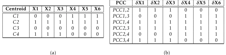
using the self-organizing map (SOM) (Kohonen, 1997), we clustered the data set and found 16 clusters, of which four were major (see Section 4.3 for details on how to identify major clusters). This meets our expectation of four major clusters corresponding to the four possibleexs. These clusters are presented in Table 1a by their centroids, which are the most prevalent patterns in the clusters, and in Table 1b by their PCCs. For example,PCC1,2, comparing clustersC1 andC2, shows that when moving fromC1to C2, only the values corresponding to variables X1, X2, and X3 have been changed (i.e.,δX1=δX2=δX3= 1
in Table 1b). Lemma 2 guarantees that the three variables are descendants of the sameEX that changed its value between twoexsrepresented byC1andC2. PCC1,4, PCC2,3, and PCC3,4reinforce this conclusion. Indeed, we know from the true graph, G1, that thisEX is latent L1. A similar conclusion can be deduced about X4, X5, and X6 as descendants of an exogenous latent, which we know, based on the true graph, is L2.
Centroid X1 X2 X3 X4 X5 X6
C1 0 0 0 1 1 1
C2 1 1 1 1 1 1
C3 0 0 0 0 0 0
C4 1 1 1 0 0 0
PCC δX1 δX2 δX3 δX4 δX5 δX6
PCC1,2 1 1 1 0 0 0
PCC1,3 0 0 0 1 1 1
PCC1,4 1 1 1 1 1 1
PCC2,3 1 1 1 1 1 1
PCC2,4 0 0 0 1 1 1
PCC3,4 1 1 1 0 0 0
(a) (b)
Table 1: (a) Centroids of major clusters for G1 and (b) PCCs between these major clusters
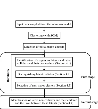
LPCC is fed by data that is sampled from the observed variables in the unknown model. LPCC clusters the data using SOM (although any other clustering algorithm is good as well), and selects an initial set of major clusters (Section 4.3). Then, LPCC learns LVM in two stages. In the first stage, LPCC first identifies exogenous latent variables and latent colliders (without distinguishing them yet) and their corresponding observed descendants (Section 4.1) before distinguishing them (Section 4.2). LPCC iteratively improves the selec-tion of the major clusters (Secselec-tion 4.3), and the entire stage is repeated until convergence. In the second stage, LPCC identifies endogenous latent non-colliders with their children. Because this stage cannot distinguish from the outset between latent non-colliders and their latent ancestors, LPCC also needs to apply a mechanism to split these two types of latent variables from each other and to find the links between them after the split (Section 4.4). A flowchart of the LPCC algorithm is given in Figure 2.
6We remind that we determined three indicators per latent in all true models we demonstrate their learn-ing (Figure 1) because BPC requires three indicators per latent to identify that latent; which makes the exper-imental evaluation we did in Part II of the paper fair.
Learning by Pairwise Cluster Comparison−Theory & Overview
Input data sampled from the unknown model
Clustering (with SOM)
Selection of initial major clusters
Identification of exogenous latents and latent
colliders and their descendants (Section 4.1)
Distinguishing latent colliders (Section 4.2)
Selection of new major clusters (Section 4.3)
Identification of latent non-colliders and their children
and the links between these latents (Section 4.4)
First stage
Second stage
It
er
at
ive
ly
4.1 Identification of exogenous latent variables and latent colliders and their descendants
Table 1b shows thatPCC1,2(andPCC3,4) provides evidence that X1, X2, and X3 may be descendants of the same exogenous latent (L1, as we know) that has changed its value between the two exs represented by C1 and C2 (and C3 and C4). Relying only on one PCC may be inadequate when concluding that these variables are descendants of the same exogenous latent because there may be other exogenous latents that have changed their values too. Table 1b shows thatPCC2,3(andPCC1,4) provides the same evidence about X1, X2, and X3. But,PCC2,3andPCC1,4also show that the values corresponding to X4, X5, and X6 have been changed together too, whereas these values did not change inPCC1,2 andPCC3,4. Does this mean that X4, X5, and X6 are also descendants of the same latent ancestor of X1, X2, and X3? If we combine the two pieces of evidence provided by, e.g., PCC1,2 and PCC2,3, we can answer this question with a “no”. This is because X4, X5, and X6 changed their values only inPCC2,3but not in PCC1,2, and thus they cannot be descendants of L1. This insight strengthens the evidence that X1, X2, and X3 are the only descendants of L1. A similar analysis usingPCC1,3andPCC2,4will identify that X4, X5, and X6 are descendants of another latent variable (L2, as we know). Therefore, we define:
Definition 16 A maximal set of observed (MSO) variables is the set of variables that always changes its values together in each major–major PCC in which at least one of the variables changes value.
That is, there is a particular interest in identifying theMSOs that always change their values together in each major–major PCC in which at least one of the variables changes value. For example, X1 (Table 1) changes its value inPCC1,2,PCC1,4,PCC2,3, andPCC3,4 and always together with X2 and X3 (and vice versa). Thus {X1, X2, X3} (and similarly {X4, X5, X6}) is anMSO. EachMSO includes descendants of the same exogenous latent variable L, and after considering all PCCs, LPCC identifies an MSOfor each exogenous latent variable.
Based on any identifiedMSO, LPCC introduces to the learned graph a new latent vari-ableLtogether with all the observed variables that are included in thisMSOas its children. At this stage, LPCC cannot yet distinguish between exogenous latents and latent colliders since the main goal at this stage is to identify latent variables. For now, LPCC focuses on the identification of the relations between the latents and the observed variables, but not on the identification of the interrelations between the latents. The latter task that is needed for distinguishing the latent colliders from the exogenous latents is performed in a further step (Section 4.2). Note, however, that the identification of endogenous latent non-colliders needs a different analysis that is based on major–minor PCCs and not on major–major PCCs, and thus it is described separately in Section 4.4.
The following Theorem 1 helps us formalize this identification step. For this theorem, we also need Definition 17 of equivalence relation/classes from set theory and Lemma 3, which is important by itself and for better understanding of LPCC, but also for proving Theorem 1.
transitive (if a∼b and b∼c, then a∼c) for all a, b, and c inA. The equivalence class of a under ∼, denoted [a], is defined as:[a] ={b∈A|bza}(Enderton, 1977).
Note that every two equivalence classes are either equal or disjoint. Therefore, the set of all equivalence classes ofAforms a partition of A; every element ofA belongs to one and only one equivalence class. It follows from the properties of an equivalence relation that: a∼bif and only if [a] = [b]. The following Lemma 3 is important since it shows that eachMSOis an equivalence class, and thusMSOs corresponding to the learned latents are disjoint. At this stage, LPCC learns a set of at least two observed variables corresponding to a specificMSOfor each latent where none of the observed variables is shared with other
MSOs for other latents; in other words, a pure measurement model.
Lemma 3 The relation “always changes together with” on the setOof all observed variables, such as “variable Oi∈O always changes together with variable O
j∈O in each PCC in which
eitherOi orOj has changed” is an equivalence relation. Each equivalence class for this relation
comprises anMSO.
Proof All three conditions that are required for a binary relation to become equivalence are met:
1. Oialways changes withOi (trivial).
2. IfOialways changes withOj, thenOj always changes withOi.
3. IfOialways changes withOj,andOjalways changes withOk, thenOialways changes withOk.
Thus, the set of observed variables in a model can be represented by a set of equivalence classes for this relation, where each equivalence class includes all the variables that have the same equivalence relation, such as anMSO.
Theorem 1 Variables of a particularMSOare children of a particular exogenous latent variable EX or its latent non-collider descendant or children of a particular latent collider C.
Note that Theorem 1 guarantees that each of multiple latent variables (either an exogenous or any of its non-collider descendants or a collider) is identified by its own MSO, regardless of the latent cardinality.
4.2 Distinguishing latent collider variables
After identifying the exogenous latents and latent colliders together (Section 4.1), we need now to separate them. To demonstrate our concept for distinguishing latent colliders, we use graph G2 in Figure 1, which shows two exogenous latent variables, L1 and L3, that collide in one endogenous latent variable, L2. We assume that all latent variables are binary,8and each has three binary observed children X1, X2, and X3 (L1), X4, X5, and X6