A Variational Approach to Path Estimation and Parameter
Inference of Hidden Diffusion Processes
Tobias Sutter [email protected]
Department of Electrical Engineering and Information Technology ETH Zurich, Switzerland
Arnab Ganguly [email protected]
Department of Mathematics Louisiana State University, USA
Heinz Koeppl [email protected]
Department of Electrical Engineering and Information Technology TU Darmstadt, Germany
Editor:Manfred Opper
Abstract
We consider a hidden Markov model, where the signal process, given by a diffusion, is only indirectly observed through some noisy measurements. The article develops a variational method for approximating the hidden states of the signal process given the full set of observations. This, in particular, leads to systematic approximations of the smoothing densities of the signal process. The paper then demonstrates how an efficient inference scheme, based on this variational approach to the approximation of the hidden states, can be designed to estimate the unknown parameters of stochastic differential equations. Two examples at the end illustrate the efficacy and the accuracy of the presented method. Keywords: Variational inference, stochastic differential equations, diffusion processes, hidden Markov model, optimal control
1. Introduction
Diffusion processes modeled by stochastic differential equations (SDEs) appear in several disciplines varying from mathematical finance to systems biology. For example, in systems biology stochastic differential equations are used for efficient modeling of the states of the chemical species in a reaction system when they are present in high abundance Wilkinson (2006). Oftentimes, the state of the system or the signal process is not directly observed, and inference of the state trajectories and parameter of the system has to be achieved based on noisy partial observations. Typically, in such a scenario, the observation data is conveniently modeled as a function of the hidden state corrupted with independent addi-tive noise. However, generalizations of this basic setup, which, for example, could include stronger coupling between the hidden signal and the observation processes, are often used for modeling more complex phenomena.
of an object needs to be constantly updated as new noisy information flows in. On the other hand, optimal smoothing involves the class of methods which can be used in reconstruction of any past state of the signal process given a set of measurements up to the present time.
More specifically, given the signal processXand the observation processY, filtering theory
entails computation of the conditional expectations of the formEφ(Xt)|FtY
, where{FY
t }
denotes the filtration generated by the process Y. The σ-algebra FtY contains all the
information about the observation processY up to the present timet. Smoothing, however,
involves evaluation of the conditional expectations of the formEφ(Xs)|FtY
, wheres < t. The smoothing techniques can also be viewed as tools of estimation of the current state given a data set which includes future observations. This interpretation is particularly relevant in statistics, where such techniques are essentially the means of computing certain posterior conditional densities given the observation set. The present article focusses on a variational approach to this smoothing problem and later employs the method for estimation of parameters of diffusion processes.
Evaluation of such conditional expectations or densities are quite difficult, since they are often solutions of suitable (stochastic) partial differential equations. These are usu-ally infinite-dimensional problems and analytical solutions are generusu-ally impossible. Hence, effort has been directed toward developing of a variety of numerical schemes for efficient approximation of these conditional densities. While Markov chain Monte Carlo methods for inference use discretization of the given SDE for writing down an approximate likelihood Kushner and Dupuis (2001); Pag`es and Pham (2005); Andrieu et al. (2010), particle meth-ods approximate the (posterior) conditional densities by suitably weighted point masses Crisan and Lyons (1999); Del Moral et al. (2001); Bain and Crisan (2009). However, these methods often rely on a suitable discretization of the problem which is mostly done in an ad-hoc way. Since a theoretical framework for obtaining approximations is not present, the approximation error might be difficult to quantify.
Instead, the present article delves much deeper in to the problem and develops methods for finding the optimal approximating SDE such that the relative entropy between it and the true posterior process is minimized subject to the condition that the marginals of the former follow Gaussian distributions. The main obstacle that needs to be overcome in this approach stems from the fact that unlike the previous case, the approximating SDE here cannot be taken to be the one with a linear drift; and a suitable expression of it needs to be found so that the marginals are still Gaussian. This has been achieved in Theorem 9. In fact, our work outlines the most general techniques for approximating the posterior density by any density from the exponential family or mixture of exponential families. In this connection we would like to note that the reason for requiring that the marginals follow a Gaussian distribution or more generally, a distribution from the exponential family because this results in a finite-dimensional smoother which can be used for approximating a wide range of distributions.
It should be noted that the variational method considered here is different from the so-called extended Kalman filter (EKF) in two ways: first, EKF is employed for filtering problems; but more importantly, EKF starts by linearizing the signal (prior) SDE and then freezing its diffusion term, while the variational approach is concerned with approximation of the posterior SDE. Therefore even though in the constant diffusion term case, the ap-proximating SDE happens to have linear drift and thus resulting in a Gaussian smoother, it is not based on the same philosophy behind the EKF. And as mentioned before, in the non-constant diffusion term case although our method can be used to obtain a finite-dimensional smoother, in particular, a Gaussian smoother, it completely avoids any form of linearization of the given SDE or subsequent freezing of the diffusion term.
In our paper this variational approximation method has been formulated as an optimal control problem. The advantage of this theoretical framework is that necessary conditions for global optimality are then obtained by employing the Pontryagin maximum principle. This leads to considerable computational advantages of the variational method compared to numerically solving the underlying (stochastic) PDEs, that is highlighted by two examples.
The later part of the paper focusses on the important topic of parameter inference of SDEs. The above scheme of estimating the hidden states and the smoothing densities is cleverly used in designing an efficient method for estimating parameters of SDEs. In particu-lar, the paper proposes an iterative EM-type algorithm which aims to compute approximate maximum likelihood estimates of the parameters in a tractable way. Two illustrative exam-ples, which are important in mathematical finance, demonstrate the accuracy and efficiency of the proposed algorithms. Future projects will address more complicated models.
process. We finally conclude with some remarks and directions for future work in Section 9. Certain technical proofs are relegated to the appendix.
Notation. Hereafter, In is the n-dimensional identity matrix and Ei is the n×nmatrix
where theii-th entry is one and zero elsewhere. We let Sym(n,R) and GL(n,R) be
respec-tively the set of symmetric and invertible n×n matrices with real entries. For matrices
A, B ∈ Rn×n let A, B := tr(A>B) denote the Frobenius inner product. For a vector
b∈Rnand a positive definite matrix A, we employ the normkbkA:=√b>A−1b. We define
the standardn−simplex as ∆n:={x∈Rn:x≥0,Pni=1xi= 1}. LetC:=C([0, T],Rn)
de-note the space of continuous functions on [0, T] taking values inRn.LetSbe a metric space,
equipped with its Borel σ-field B(S). The space of all probability measures on (S,B(S)) is
denoted by P(S). The relative entropy (or Kullback-Leibler divergence) between any two
probability measures µ, ν ∈ P(S) is defined as
D µ||ν:=
( R
logdµdνdµ, ifµν
+∞, otherwise,
wheredenotes absolute continuity of measures and dµdν is the Radon-Nikodym derivative.
By conventionmeasurablemeansBorel-measurable in the sequel. Given anS-valued random
variableX with Law(X) =µ∈ P(S), letEµ
Xdenote the expectation of X.
2. Model setup
As usual, we will work on a complete probability space (Ω,F,P) equipped with a filtration
{Ft}satisfying the usual conditions, that is,{Ft}is complete, right continuous and contains
all the P-null sets. The basic objects in our study consist of a signal process X and an
observation process Y, both of which are assumed to be {Ft}- adapted. The unobserved
signal processX is modeled by the following stochastic differential equation describing the
state evolution of a dynamical system:
dXt=f(Xt)dt+σ(Xt)dWt, X0 =x0, 0≤t≤T, (1)
where f : Rn → Rn, σ : Rn → Rn×n, and W is an n-dimensional Brownian motion
independent of x0. The observation processY is modeled as noisy measurements of some
function of the signal processX. Mathematically, Y is defined as
Yt= Z t
0
h(Xs)ds+Bt, (2)
whereh:Rn→Rm is called the observation function andB is anm-dimensional Brownian
motion independent of x0 and W.
Assumption 1 We stipulate that
(i) f and σ are globally Lipschitz;
It is known Kallenberg (2002) that under Assumption 1 there exists a unique strong solution
to the SDE (1). Given the observed data up to some time T,{Ys:s≤T}, the goal of the
paper is to outline an approximation method for the smoothing density, PS(x, t), which is
the conditional probability density ofXtgiven{Ys:s≤T}. In other words, the smoothing
density is defined by the equation:
Eφ(Xt)|FTY
=
Z
φ(x)PS(x, t) dx, (3)
up to a.s. equivalence, where φ is any bounded measurable function from Rn to R and
{FtY}denotes the filtration generated by the processY.
More generally, we will be interested in approximating the full conditional probability
measure on the path space,C ≡C([0, T],Rn). To describe this mathematically, assume that
a regular conditional probability measure P·|FTY
is chosen. Then there exists a measurable
probability kernel y∈ C →Πpost(·, y)∈ P(C) such that for any measurable setA ⊂ C,
PX[0,T]∈ A|FTY
= Πpost(A, Y[0,T]).
Given the observation process up to timeT,Y[0,T], we now describe a characterization of
the probability measure Πpost(·, Y[0,T]), which will play a pivotal role for our purposes. The
probability measure Πpost(·, Y[0,T]) is actually the distribution of a diffusion process ¯XT on
C, and the latter is obtained by a modification of the original signal processX:
dX¯tT =g( ¯XtT, t)dt+σ( ¯XtT)dW¯t, X¯0T =x0, (4)
where ¯W is an {Ft}-adapted Brownian motion that is independent of Y. Notice that the
diffusion coefficient of the above SDE (which we will henceforth call the posterior SDE or posterior diffusion) is same as that of the original SDE, and the drift of this posterior SDE is time-dependent and is obtained as
g(x, t) :=f(x) +a(x)∇logw(x, t), (5)
wherea(x) :=σ(x)σ(x)>. We give details about the (random) functionwa little later, but
the important point to note here is that the new drift function is the old drift function with
an extra additive term, and the observation process Y[0,T] enters into the characterization
of Πpost(·, Y[0,T]) only throughw.
To see this characterization of Πpost(·, Y[0,T]), we first look at the usual filtering density
PF(x, t), which is naturally defined by
Eφ(Xt)|FtY
=
Z
φ(x)PF(x, t) dx. (6)
Under suitable technical conditions, the filter densityPF satisfies the Kushner-Stratonovich
equation (for example, see Stratonovich (1960); Kushner (1967); Bain and Crisan (2009)). For our purposes, however, it is convenient to work with the unnormalized filter density p(x, t), that is,PF(x, t) =p(x, t)(R
Rnp(x, t)dx)
−1, which satisfies the so-called Zakai
equa-tion Zakai (1969) (
dp(x, t) =A∗p(x, t)dt+p(x, t)h(x)>dY
t
p(x,0) =p0(x).
Herep0 denotes the density ofx0 andA∗ is the adjoint of the infinitesimal generator of the
processX given byAψ(x) =Pifi(x)∂x∂iψ(x) +12Pi,jai,j(x) ∂
2
∂xi∂xjψ(x) forψ∈ C 2
0(Rn,R).
We next consider the backward stochastic partial differential equation (SPDE)
(
dw(x, t) =−Aw(x, t)dt−w(x, t)h(x)>dY
t
w(x, T) = 1. (8)
Conditions about existence of solutions to (7) and (8) can be found in Pardoux (1981/82). It is well known (Pardoux, 1981/82, Corollary 3.8) that the smoothing density can be expressed as
PS(x, t) = R p(x, t)w(x, t)
Rnp(x, t)w(x, t)dx
. (9)
Now by using (7), (8) and (9), it can be shown1 that the smoothing density solves the
following Kolmogorov forward equation
∂
∂t+
X
i
∂ ∂xi
g(x, t)−1 2
X
i,j
∂2
∂xi∂xj
aij(x)
PS(x, t) = 0, (10)
with the drift term g defined by (5). In other words, the conditional probability measure
Πpost(·, Y[0,T]) on C is induced by the diffusion process ¯XT as defined in (4).
Evaluating Πpost(·, Y[0,T]) is what is known as the path estimation problem. Except for
a few simple cases, the SPDEs, that are involved in this estimation of the hidden path, are analytically intractable. The variational approach that we undertake in this paper actually
has the goal of approximating Πpost(·, Y[0,T]). Toward this end, a natural objective is to
approximate Πpost(·, Y[0,T]) by a probability measure such that the corresponding marginals
of the latter come from a known family of distributions (e.g, exponential family). As a
result, the marginal of this approximating probability measure at time tapproximates the
smoothing density PS(x, t). The procedure adopted in this article involves finding the
optimal parameters of this approximating distribution by minimizing the relative entropy between the posterior distribution and the approximating one.
2.1 Example: Geometric Brownian Motion
We present as a running example throughout the article the geometric Brownian motion that is used to model stock prices in the Black-Scholes model, see Shiryaev (1999). The system dynamics (1) is given by a one-dimensional geometric Brownian motion
dXt=κXtdt+λXtdWt, X0=x0 ∼logN(µ, σ), (11)
for 0≤t≤T,λ, κ >0 and an observation process (2) defined by
Yt= Z t
0
Xsds+Bt. (12)
It is straightforward to see that Assumption 1 holds in this setting.
3. Variational approximation: Motivation
Let Πprior denote the distribution of the original signal process X on C, that is, for a
measurable A ⊂ C, Πprior(A)≡ PX[0,T]∈A
. Define the two terms
HT(X[0,T], y) :=−h(XT)yT + Z T
0
ysdh(Xs) +
1 2
Z T 0 k
h(Xs)k2ds (13)
I(HT(·, y)) :=−log Z
exp (−HT(·, y)) dΠprior
. (14)
Letybe a sample path of the observation processY on the interval [0, T]. Then notice that
by the pathwise Kallianpur-Striebel formula (or the Bayes formula), we have
dΠpost(·, y)
dΠprior
= R exp(−HT(·, y))
exp(−HT(·, y))dΠprior
= exp(−HT(·, y))
L(y) .
where L(y) = R exp(−HT(·, y))dΠprior. Consequently, L(y) can be interpreted naturally
as the likelihood of the path y, or equivalently, I(HT(·, y)) is viewed as the negative
log-likelihood of the sample path y. The term HT(X[0,T], y) can be interpreted as the X
-conditional information and the information in the observation that Y =y, see Mitter and
Newton (2003) for more details. Now for any probability measure Q2 on C([0, T],R), the
relative entropy betweenQand Πpost(·, y) can be expressed by the following lemma.
Lemma 2 D Q||Πpost(·, y)=−I(HT(·, y)) +D Q||Πprior+EQ
HT(·, y).
Proof. The proof essentially follows the one in (van Handel, 2007, Lemma 2.2.1). Splitting
the relative entropy and using the pathwise Kallianpur-Striebel formula yields
D Q||Πprior= Z
log
dQ
dΠpost(·, y)
+ log
dΠpost(·, y)
dΠprior
dQ
=D Q||Πpost(·, y)+ Z
log
dΠpost(·, y)
dΠprior
dQ
=D Q||Πpost(·, y)
+
Z
log
exp(−HT(·, y)) R
exp(−HT(·, y))dΠprior
dQ
=D Q||Πpost(·, y)−EQ
HT(·, y)−log Z
exp(−HT(·, y))dΠprior
.
Mitter and Newton Mitter and Newton (2003) provide an information-theoretic
interpre-tation to this result. They interpret the term (14) as the total information available to
the estimator Q through the sample path y. On the other hand, they call the quantity
F(Q, y) := D Q||Πprior
+EQ
HT(·, y)
the apparent information of the estimator. By
non-negativity of the relative entropy F(Q, y) ≥ I(HT(·, y)) with equality if and only if
Q = Πpost(·, y). In this sense, a suboptimal estimator appears to have access to more
information than is actually available.
Since the total information I(HT(·, y)) does not depend on Q, minimizing the relative
entropy between Q and Πpost(·, y) over a class of probability measures Q is equivalent to
minimizing the apparent informationF(Q, y). This motivates to consider an approximating
distribution Q on C that is characterized as the solution to the following optimization
problem:
Problem 3 MinimizeD Q||Πprior
+EQ
HT(·, y)
subject to
(i) Q is a probability distribution induced by an SDE of the form
dZt=u(Zt, t)dt+σ(Zt)dWt, Z0 =x0, 0≤t≤T; (15)
(ii) The marginals ofQ at timet, i.e., the distribution of Zt, belong to a chosen family of
distributions.
We will show in the remainder of this article how Problem 3 can be restated as an optimal control problem, which leads to a standard formulation of necessary optimality conditions in terms of Pontryagin’s maximum principle.
Note that the objective function of Problem 3 is known to be strictly convex with
re-spect to Q, see Csisz´ar (1975). The constraint (ii) restricts the feasible set approximating
distributionsQto a nonconvex set. Note that such problems (i.e., absence of constraint (i)
have been studied in the literature Pinski et al. (2015)). In our setting, the set of feasible solutions is also coupled with the first constraint (i), that parametrizes the feasible set of
distributions in terms of the drift functionu. This coupling is investigated in Section 4, in
particular Theorem 9 characterizes the set of all drift terms u such that the distribution
induced by (15) has finite dimensional marginals that belong to a given family of distri-butions. Hence, Problem 3 can alternatively be interpreted as minimizing the objective
function over a class of drift functions u that induce Q via (15) and such that Q satisfies
constraint (ii). For example, if the goal is to approximate the posterior distribution Πpost
by a distribution Qwhose marginals are normal distributions, then one aims to find a drift
termu such that the objective function is minimized and such that the solutionZt to (15)
admits a normal distribution.
Remark 4 Notice that the unconstrained optimization of the objective function in Problem
3 with respect to Q will simply yield the minimizer Q to be Πpost. Since, as discussed in
the beginning of Section 2, Πpost is induced by the SDE, (4), the constraint (i) in Problem
3 is essentially inbuilt. In other words, it is the constraint (ii) which plays the crucial role
in the methods outlined in this paper.
The objective function in Problem 3, in particular the relative entropy between the
approx-imating distributionQ and the prior distribution Πprior can be simplified, since due to the
constraint (i) the underlying SDEs (15) and (1) share the same diffusion coefficient. In view
of (15) and (1), consider two SDEs for 0≤t≤T
dXt=f(Xt)dt+σ(Xt)dWt, dZt=u(Zt, t)dt+σ(Zt)dWt, X0=Z0 =x0,
withu:Rn×R→Rn, f :Rn→Rn, σ:Rn→Rn×n, W ann-dimensional Brownian motion
space, where FT is the sigma algebra σ(Ws :s ≤T) and let Πprior and Q denote the the
laws of Xt and Zt with respect to P. It follows by Girsanov’s Theorem Øksendal (2003),
that
EQ
log
dQ
dΠprior
= 1
2EQ
Z T 0
ϕ(s, ω)>ϕ(s, ω)ds
,
where ϕ(s, ω) := σ(Zs(ω))−1(u(Xs(ω))−f(Xs(ω))). Therefore, the relative entropy
be-tweenQ and Πprior is
D Q||Πprior= 1
2EQ
Z T 0 k
u(Xs, s)−f(Xs)k2a(Xs)ds
,
where ku(x, s)−f(x)k2a(x) := (u(x, s)−f(x))>a(x)−1(u(x, s)
−f(x)). Hence, the
objec-tive function in Problem 3 can be expressed as
D Q||Πprior+EQ
HT(·, y)
=
Z T 0 EQ
1
2ku(Xt, t)−f(Xt)k
2
a(Xt)+yt
u(Xt, t)>∇h(Xt)
+1
2σ(Xt)
>∇2h(X
t)σ(Xt)
+ 1
2kh(Xt)k
2
dt−yTEQ
h(XT),
(16)
where the last equality is due to Fubini’s Theorem and Itˆo’s Lemma. The two coupling
constraints (i) and (ii) in Problem 3 are studied in the next section and will finally allow us to reformulated Problem 3 as an optimal control problem.
4. Multi-dimensional SDE with prescribed marginal law
This section establishes conditions on the drift function in the approximate SDE (15) such that the induced marginal distributions evolve in a given exponential family.
Definition 5 (Exponential family) LetH1, . . . ,Hmbe Hilbert spaces and letH=Qmi=1Hi
be endowed with the inner product ·,·. Let the functionsci:Rn→ Hi for i= 1, . . . , m be
linearly independent, have at most polynomial growth, be twice continuously differentiable
and denote c(x) = (c1(x), . . . , cm(x)). Assume that the convex set
Γ :=Θ∈ H : ψ(Θ) = logRexp Θ, c(x)dx <∞ has non-empty interior. Then
EM(c) ={p(·,Θ),Θ∈Λ}, p(x,Θ) := exp Θ, c(x)−ψ(Θ),
where Λ⊆Γ is open, is called an exponential family of probability densities.
Definition 6 (Mixture of exponential families) Let EM(c(i)) for i= 1, . . . , k be expo-nential families according to Definition 5. Then
EM(c(1), . . . , c(k)) =
Xk
`=1
ν`p`(·,Θ(`)) : p`(·,Θ(`))∈EM(c(`)), ν ∈∆k
Consider the stochastic differential equation (15), whereu :Rn×R→Rn,σ :Rn→Rn×d
and W is ad-dimensional Brownian motion independent ofx0.
Assumption 7
1. The SDE (15) satisfies Assumption 1.
2. The initial conditionx0 has a densityp0 that is absolutely continuous with respect to
the Lebesgue measure and has finite moments of any order.
3. The unique solution Xt to (15) admits a density p(x, t) that is absolutely continuous
with respect to the Lebesgue measure and that satisfies the Kolmogorov forward equation.
Problem 8 Let EM(c(1), . . . , c(k)) be a mixture of exponential families, let p0 be a density
contained in EM(c(1), . . . , c(k)), let σ be a diffusion term and let a(·) := σ(·)σ(·)>. Let
U(x0, σ) denote the set of all driftsu such that x0, u, σ and its related SDE (15) satisfy
As-sumption 7. Assume U(x0, σ) to be non-empty. Then given a curve t7→p(·,Θ(1)t , . . . ,Θ
(k) t )
in EM(c(1), . . . , c(k)), find a drift inU(x0, σ)whose related SDE has a solution with marginal
density p(·,Θ(1)t , . . . ,Θ(k)t ).
A solution to Problem 8 is given by the following theorem.
Theorem 9 Given the assumptions and notation of Problem 8. Consider the SDE (15)
with drift term
ui(x, t) =
1 2
n X
j=1
∂ ∂xj
aij(x) +
1 2
n X
j=1
aij(x) ∂
∂xjp(x,Θ (1) t , . . . ,Θ
(k) t )
p(x,Θ(1)t , . . . ,Θ(k)t )
− 1
p(x,Θ(1)t , . . . ,Θ(k)t )
k X
`=1
ν`p`(x,Θ(`)t ) D
˙
Θ(`)t ,Ii(`)(x)E,
for i= 1, . . . , n, where
Ii(`)(x) := Z xi
−∞
ϕ(`)i ((x−i, ξi),Θ(`)t ) exp D
Θ(`)t , c(`)(x−i, ξi)−c(`)(x) E
dξi, (17)
(xi−, ξi) := (x1, . . . , xi−1, ξi, xi+1, . . . , xn)> and the functions ϕ(`)i : Rn× H → H for all
`= 1, . . . , k satisfy
n X
i=1 D
˙
Θ(`)t , ϕ(`)i (x−i, ξi),Θ(`)t E ξi=xi
=DΘ˙(`)t , c(`)(x)− ∇Θψ`(Θ(`)t ) E
. (18)
If u∈ U(x0, σ), then the SDE (15) solves Problem 8, i.e.,Xt has a density
pXt(x) = k X
`=1
ν`exp D
Θ(`)t , c(`)(x)E−ψ`(Θ(`)t )
The proof is provided in Appendix B.
Remark 10 1. For the non-mixture and one-dimensional case (k =n= 1), the result is known Brigo (2000) and coincides with Theorem 9. Furthermore, it can be seen by the proof in Brigo (2000) and by invoking the existence and uniqueness theorem for
ODEs, that the drift functionu is uniquely determined.
2. For the multi-dimensional case (n >1), the drift function is not unique anymore, as
there exist multiple choices for ϕ(`)i 3. This gives rise to a natural question, if there
exist a particular choice ofϕ(`)i such that the integral termsIi(`) in (17) admit
closed-form expressions. In Section 4.1 (Proposition 11), we derive such functions ϕ(`)i for
the mixture of multivariate normal densities.
3. In a non-mixture setting (k= 1), the drift function simplifies to
ui(x, t) =
1 2
n X
j=1
∂ ∂xj
ai,j(x) +
1 2
n X
j=1
ai,j(x)
Θt,
∂c(x) ∂xj
−
˙ Θt,
Z xi
−∞
ϕi((x−i, ξi),Θt) expΘt, c(x−i, ξi)−c(x)dξi
,
where the functionsϕi have to satisfy (18).
As remarked, the drift term proposed in Theorem 9 consists of the integral terms (17), that depend on the particular exponential families considered. In the following, we restrict ourselves to the mixture of multivariate normal densities and show that these integral terms, and hence the drift function, admit a closed-form expression.
4.1 Mixture of multivariate normal densities
Consider the family of multivariate Gaussian distributions with mean m∈Rn and
covari-ance matrix S ∈Sym(n,R), that can be expressed in terms of Definition 5 as follows. Let
the Hilbert space H = Rn×Rn×n be endowed with the inner product (a, A),(b, B) =
a>b+tr(A>B) and define
Θ = (η, θ) :=
S−1m,−1
2S
−1
∈ H, c:Rn→ H, c(x) = (x, xx>)
ψ:H →R, ψ(Θ) =−1
4tr(ηη
>θ−1) +1
2log det
−12θ−1
+n
2 log(2π).
(19)
A direct computation, usingtr(ηη>θ−1) =η>θ−1η, leads to
p(x,Θ) = exp c(x),Θ−ψ(Θ)= 1
(2π)n2(detS)12 exp
−12(x−m)>S−1(x−m)
.
3. For example,ϕ(i`)(x,Θt(`)) :=δij(c(`)(x)− ∇Θψ`(Θt(`))) for allj∈ {1, . . . , n}are feasible choices forϕ
(`)
We point out again that for the proposed variational method, it is favourable if the approx-imating SDE (15) has a drift function that admits a closed-form expression. Furthermore, since the drift function is not unique (cf. Remark 10), among all feasible solutions
char-acterized by the ϕ(`)i functions, we want to find one that can be computed analytically.
The latter turns out to be a difficult task and depending heavily on the specific exponential familiy chosen. From now on, we consider the exponential family of the multivariate normal probability densities that is given by (19). In this setting, it is possible to find functions
ϕ(`)i such that the integral terms (17), and therefore the drift function, can be computed in
closed form.
Proposition 11 For the mixture of multivariate normal densities, one possible choice for the drift function proposed by Theorem 9 is
u(x, t) = 1
2div a(x)
+
Pk
`=1ν`p`(x,Θ(`)t )
p(x,Θ(1)t , . . . ,Θ(k)t )
1 4θ
(`) t
−1
˙
θ(`)t θ(`)t −1ηt(`)−1
2θ
(`) t
−1
˙ ηt(`)
−1
2θ
(`) t
−1
˙
θ(`)t x+a(x)
1 2η
(`) t +θ
(`) t x
.
The proof is provided in Appendix C.
Remark 12 For the non-mixture setting the drift term simplifies to u(x, t) = 1
2div a(x)
+ 1
4θ
−1
t θ˙tθt−1ηt−1
2θ
−1 t η˙t−1
2θ
−1
t θ˙tx+a(x)
1
2ηt+θtx
,
that in the special case of a constant diffusion term is a linear function, as one would expect.
We introduce the following ansatz for the drift function
u(x, t) =1
2div a(x)
+
Pk
`=1ν`p`(x,Θ(`)t )
A(`)t +Bt(`)x+a(x)Ct(`)+D(`)t x
p(x,Θ(1)t , . . . ,Θ(k)t ) ,
(20)
where Bt(`), D(`)t ∈Rn×n and A(`)t , C (`)
t ∈Rn for all`= 1, . . . k. The coefficients A
(`) t ,B
(`) t ,
Ct(`) and D(`)t cannot be chosen arbitrarily. They are coupled according to Proposition 11.
By comparing the coefficients of Proposition 11 and (20) one gets
A(`)t =1 4θ
(`) t
−1
˙
θ(`)t θ(`)t −1ηt(`)− 1
2θ
(`) t
−1
˙
η(`)t , Bt(`)=−1
2θ
(`) t
−1
˙
θt(`), Ct(`)=1 2η
(`) t , D
(`) t =θ
(`) t .
Hence, one directly sees that the four parametersA(`)t ,B(`)t ,Ct(`)andDt(`)for all`= 1, . . . , k
are coupled via the two ODEs
dCt(`)
dt =−D
(`) t A
(`) t −B
(`) t
>
Ct(`), dD
(`) t
dt =−2D
(`) t B
(`)
t . (21)
4.2 Equations for mean and variance
Theorem 9 provides an explicit formula for the drift term in the approximating SDE (15), that simplifies to (20) in the case of multi-normal marginal densities. Therefore, the mean and variance of the approximating SDE (15) are characterized via the following two ODEs.
Theorem 13 Consider the SDE (15)with drift termugiven by (20), such that the solution
Xt has a marginal density p(x,Θ(1)t , . . . ,Θ
(k)
t )∈EM(c1, . . . , ck) that is an arbitrary convex
combination of densities p`(x,Θ(`)t )∈EM(c`) for `= 1, . . . , k. Letm(`)t andS
(`)
t denote the
mean and variance of Xt with respect top`(x,Θ(`)t ). Then,
dm(`)t
dt =
1 2Ep`
div a(X)+A(`)t +Bt(`)m(`)t +Ep`
a(X)Ct(`)+Ep` h
a(X)D(`)t Xi (22)
and
dSt(`)
dt =
1 2Ep`
h
Xdiv a(X)>i+ 1 2Ep`
div a(X)X>−1
2m
(`) t Ep`
div a(X) >
−1
2Ep`
div a(X) m(`)t >+Ep`
a(X)+St(`)Bt(`)>+Bt(`)St(`) +Ep`
h
XCt(`)>a(X)i+Ep` h
a(X)Ct(`)X>i−m(`)
t C (`) t
>
Ep`
a(X) (23)
−Ep`
a(X)Ct(`)m(`)t >+Ep` h
XX>D(`)
t a(X) i
+Ep` h
a(X)D(`)t XX>i
−m(`)t Ep` h
X>D(`)
t a(X) i
−Ep` h
a(X)D(`)t Xim(`)t >.
The proof is provided in Appendix D. Note that givenm(`)t and St(`)the mean and variance
of Xt can be expressed as mt = Pk`=1ν`mt(`) and St =Pk`=1ν`S(`)t +
Pk
`=1ν`m(`)t m (`) t
>
−
(Pk`=1ν`m(`)t )( Pk
`=1ν`m(`)t )>, respectively.
Remark 14 If the coefficientsνi in the convex combination of the marginal density
p(x,Θ(1)t , . . . ,Θ(k)t ) in Theorem 13 are fixed a priori, the ODEs (22) and (23) are only
sufficient for describing m(`)t and St(`). Oftentimes, however, one is interested in choosing
those coefficients a posteriori, for example by solving an auxiliary optimization problem. In such a setting the ODEs given by Theorem 13 are necessary and sufficient.
We have studied how to reformulate the constraints (i) and (ii) of Problem 3 by deriv-ing an expression for the drift term to the approximatderiv-ing SDE (15). In the case that the marginals in (ii) are restricted to a mixture of multivariate normal densities this reformu-lation reduces to the ODEs (21), (22) and (23).
4.3 Example: Geometric Brownian Motion
We continue the geometric Brownian motion example started in Section 2.1. The goal is to approximate the smoothing density by a normal density. Therefore, according to Proposition 11, the drift function for the approximating SDE (15) has to be chosen as
where the coefficientsAt, Bt, Ct, Dt are coupled via the two ODEs (21). This choice of drift
function leads to ODEs for the mean and the variance of the posterior process, according to Theorem 13
dmt
dt =λ
2m
t+At+Btmt+λ2Ct(m2t+St) +λ2Dt(m3t+ 3mtSt) (25)
dSt
dt =λ
2(m2
t + 3St) + 2BtSt+ 4λ2CtmtSt+ 6λ2Dt(m2tSt+St2). (26)
5. Optimal control problem formulation
In this section, we show that the optimization problem 3, using the results derived from Theorem 9, can be reformulated as a standard optimal control problem (OCP), which
conceptually is similar to Mitter and Newton (2003)4. Therefore, the presented variational
approximation method to the path estimation problem for SDEs can be expressed as an OCP and as such leads to a standard formulation of necessary global optimality conditions
in terms of Pontryagin’s maximum principle. Consider the vector spaces ˆV :=Rn×Rn×n,
ˆ
Z :=Rn×Sym(n,R)×Rn×Sym(n,R) and define the trajectories
[0, T]3t7→v(`)(t) := (A(`)t , Bt(`))∈Vˆ
[0, T]3t7→z(`)(t) := (m(`)t , S(`)t , Ct(`), Dt(`))∈Zˆ,
for`= 1, . . . , k. We introduce the state variablez(t) := z(1)(t), . . . , z(k)(t) ∈Qk
`=1Zˆ=:Z
and the control variablev(t) := v(1)(t), . . . , v(k)(t)∈Qk
`=1Vˆ =:V fort∈[0, T]. As a first
step, in view of the cost functional (16) of Problem 3, the so-called Lagrangian
EQ
1
2ku(Xt, t)−f(Xt)k
2 a(Xt)
+yt
u(Xt, t)>∇h(Xt) +
1 2σ(Xt)
>∇2h(X
t)σ(Xt)
+ 1
2kh(Xt)k
2
(27)
is expressed as a function of only z(t), v(t) and t. This step, while being exact in some
cases, may require an approximation. In the case that the marginals of Q are mixtures of
normal densities, the expectation of any polynomial inXtcan be expressed as a function of
its mean and variance. If the diffusion termσis a polynomial, and no mixture is considered
(k = 1), the drift function u, according to (20), is a polynomial. We refer to Section 8 to
see how the Lagrangian can be derived for two concrete examples. Consider a Lagrangian
L: [0, T]× Z × V →R, L(t, z(t), v(t))≈(27),
where≈indicates that in order to express the term (27) by the state and control variables
only, an approximation might be needed, as explained above. Similarly to the Lagrangian,
in view of the cost functional (16), we introduce a terminal costF :Z →Rby
F(z(T))≈ −yTEQ
h(XT).
Under the assumption that the drift term σ is a polynomial, the ODEs derived in the
previous section can be expressed in standard form. We define the functionH:Z × V → Z
by
H(z(t), v(t)) =H1(1)(z(t), v(t)), . . . , H4(1)(z(t), v(t)), . . . , H1(k)(z(t), v(t)), . . . , H4(k)(z(t), v(t)), where
dm(`)t
dt =
dz(`)1
dt (t) =H
(`)
1 (z(t), v(t)),
dCt(`)
dt =
dz(`)3
dt (t) =H
(`)
3 (z(t), v(t)),
dSt(`)
dt =
dz(`)2
dt (t) =H
(`)
2 (z(t), v(t)),
dD(`)t
dt =
dz4(`)
dt (t) =H
(`)
4 (z(t), v(t)),
for`= 1, . . . , kare given by (22), (23) and (21). Thus, we have shown so far in this article that Problem 3 can be reformulated as the following optimal control problem
minimize
v∈M([0,T],V) J(v) = RT
0 L(t, z(t), v(t))dt+F(z(T))
subject to z˙(t) = H(z(t), v(t)), t∈[0, T] a.e.
z(0) = z0,
(28)
where M([0, T],V) denotes the space of measurable functions from [0, T] toV. It remains
to discuss how to find the initial conditionz0 in the OCP (28). A straightforward, however,
clearly not efficient, method for that is solving the Pardoux equation (8), which according
to (9) provides the smoothing density at initial time as PS(x,0) = R p0(x)w(x,0)
Rnp0(x)w(x,0)dx
, from
wherez0 can be derived.
5.1 Maximum principle
We derive necessary conditions for global optimality of the optimization problem (28) that
are provided by the Pontryagin maximum principle (PMP). Since the control set V is
un-bounded, we need an extended setting of the standard PMP, see (Clarke, 2013, Section 22.4) for a comprehensive survey. It requires some further assumptions.
Assumption 15 Let the process (z?(t), v?(t))
t∈[0,T]be a local minimizer for the OCP (28),
that satisfies
(i) The functionF is continuously differentiable;
(ii) The functions H and L are continuous and admit derivatives relative to z which are
themselves continuous in all variables (t, z, v);
(iii) There existε >0, a constantc, and a summable functiondsuch that for almost every
t∈[0, T], we have
Note that Assumption 15(iii) is implied if
|∇zH(t, z, v)|+|∇zL(t, z, v)| ≤c(|H(t, z, v)|+|L(t, z, v)|) +d(t)
holds for allv ∈ V whenzis restricted to a bounded set, which is satisfied by many systems.
Moreover, the condition automatically holds ifv? happens to be bounded.
Lemma 16 (PMP (Clarke, 2013, Theorem 22.2)) Given Assumption 15, let the pro-cess (z?(t), v?(t))t∈[0,T] be a local minimizer for the problem (28). Then there exists an
absolutely continuous function p: [0, T]→ Z satisfying
1. the adjoint equation p˙(t) =−∇zp(t), H(z?(t), v?(t))−∇zL(t, z?(t), v?(t))for almost
every t∈[0, T];
2. the transversality condition p(T) =∇zF(z(T));
3. the maximum condition
p(t), H(z?(t), v?(t))+L(t, z?(t), v?(t)) = inf v∈V
p(t), H(z?(t), v)+L(t, z?(t), v) for
almost everyt∈[0, T].
Remark 17 1. Given that an optimal process (z?, v?) exists5, the maximum condition 3 can be used to derive a feedback law
v?(t)∈arg min
v∈V
p(t), H(z?(t), v)+L(t, z?(t), v).
2. Lemma 16, basically leads to a boundary value problem with initial conditions for the states and terminal conditions for the adjoint states, that provides necessary conditions for global optimality of Problem 3.
We summarize the described method to approximate the smoothing density introduced so far. It basically consists of the following three steps, that provide a solution to Problem 3:
Step 1 Fix a mixture of exponential families of probability densities, e.g., the mixture of multivariate normal densities. Theorem 9, that simplifies to Proposition 11 for the multivariate normal densities, characterizes the approximate posterior SDE (15) whose solution admits marginal densities evolving in the chosen mixture of exponential fam-ilies.
Step 2 Given the approximate posterior SDE (15), we derive an optimal control formulation of Problem 3. For the mixture of multivariate normal densities, this derivation is presented in Sections 4 and 5 and finally leads to the OCP (28).
Step 3 Necessary conditions for optimality of the OCP (28), and hence for Problem 3, can be derived from Pontryagin’s maximum principle and result in a structured boundary value problem.
Remark 18 It is important to note that the presented method chooses the best approxi-mating SDE in a desired class using an objective distance measure between the correspond-ing probability distributions. One crucial advantage of this approach is that this distance could be quantified and numerically calculated (note that the first term in Lemma 2 can be directly computed and the remaining two terms form the objective function of the op-timal control problem considered), and hence the user gets an excellent estimate on the necessary approximating error. For instance, Figure 1d and Figure 2d demonstrated the accuracy of corresponding approximating SDEs by plotting the relative entropies between the approximate models and the exact ones for the two examples considered in the paper.
5.2 Computational complexity
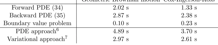
If the initial condition to the OCP (28) is known, the PMP, Lemma 16, reduces to a bound-ary value problem, that can usually be solved numerically more efficiently than (S)PDEs by using numerical methods specifically tailored to these problems, such as the shooting method, see Stoer and Bulirsch (2002). Therefore, the major computational difficulty of the presented variational approach lies in estimating the initial condition to the OCP (28), for example via estimating the smoothing density at initial time. A straightforward, how-ever clearly not efficient, method for that is solving the Pardoux equation (8), as explained in Section 2, which we used in the numerical examples in Section 8. As such, whereas the standard PDE approach for computing a smoothing density requires solving a Zakai equation and the Pardoux equation (8), the presented variational approach relies on only a Pardoux equation and the mentioned boundary value problem. This can usually be seen as a reduction in terms of computational effort required and is demonstrated by two numerical examples in Section 8, Table 1. Moreover, for future work, we aim to study the derivation of an estimator for the marginal smoothing density at terminal time without solving a Pardoux equation, that would then allow us to apply the proposed variational approximation method to high-dimensional problems, see Section 9 for more details. Another idea to circumvent the estimation of this mentioned terminal condition is to use an alternative approach to the PMP, for characterizing a solution to the OCP (28) that is briefly described in the following remark.
Remark 19 (Semidefinite programming) Solutions to the OCP (28) can be charac-terized via the so-called weak formulation which consists of an infinite-dimensional linear program, see (Lasserre, 2010, Chapter 10) for details. Therefore, numerical approximation schemes to such infinite-dimensional linear programs, that have been studied in the liter-ature, can be employed to solve Problem 3. This approach seems particularly promising when the data of the OCP (dynamics and costs) are described by polynomials, as then the seminal Lasserre hierarchy based on solving a sequence of semidefinite programs, is applicable Lasserre (2001, 2010).
5.3 Example: Geometric Brownian Motion
We continue the geometric Brownian motion example started in Sections 2.1 and 4.3 and formulate the corresponding optimal control problem (28). Recall that the state variable is
the state variables are given by (21), (25) and (26). The objective function of the optimal
control problem (28) can be expressed asF(x(T)) =−yTmT and
L(t, z(t), v(t)) = A
2 t
2λ2(m2 t +St)
+ At(λ
2+B t−κ)
λ2m t
+(λ
2+B t−κ)2
2λ2 +AtCt+ytAt
+mt Ct(λ2+Bt−κ) +AtDt+yt(λ2+Bt)
+ (m2t +St)
1
2λ
2C2
t +Dt(λ2+Bt−κ) +
1
2 +λ
2y tCt
+ (m3t + 3mtSt) λ2CtDt+λ2ytDt+ (m4t+ 6m2tSt+ 3St2)
λ2
2 D
2 t,
where, in order to derive the cost function above, the first two inverse moments ofXtwith
respect to Qhave been approximated. Due to the non-negativity of the GBM, we use the
approximation EQXt−1
≈ EQXt−1 = m−t1 and EQ
Xt−2 ≈ EQXt−2 = (St+m2t)−1,
whose accuracy has been investigated in Garcia and Palacios (2001).
6. Parameter inference
The goal of this section is to outline the use of the techniques, developed so far for path estimation, for inference of parameters in a hidden Markov model. We consider a class of dynamical systems
dXtκ=f(Xtκ, κ)dt+σ(Xtκ, κ)dWt, X0κ =x0, 0≤t≤T, (29)
parametrized byκ. The observation process can be modeled by (2), but as discussed in the
next section, the approach discussed below can also be used with necessary modifications for a discrete observation process.
As a natural notation, for each parameter κ, the probability distribution of X[0,Tκ ] on
C will be denoted by Πκprior. Given a sample path {yt : 0 ≤ t ≤ T} of the
observa-tion process Y[0,T], the objective is to select an optimal κ? ∈ Rd such that the
obser-vation process (Yt)t∈[0,T] in (2) has a high probability of reproducing the given data y.
This is basically the inference scheme based on classical maximum likelihood estimation,
and we propose an algorithm similar to the lines of expectation maximization (EM)
algo-rithm (see Capp´e et al. (2005) for a comprehensive survey), which aims to obtain the
op-timal κ? through multiple iterations. Recalling (14), for eachκ, we defineIκ(H
T(·, y)) := −logR exp (−HT(·, y)) dΠκprior
. As already noted in Section 3, for each parameterκ, the
termIκ(HT(·, y)) provides the total information available through the sample path y, and
can be interpreted as the negative log-likelihood ofygiven the parameterκ. However,
min-imizing this negative log-likelihood function, even if numerical evaluation of it can be done, usually is a hard problem. But, as mentioned in Section 3, Lemma 2 and non-negativity of the relative entropy together imply that an upper bound to this negative log-likelihood
term is given by the apparent information,F(Q, κ) :=D
Q||Πκprior+EQ
HT(·, y)
. The ad-vantage of this observation is that this upper bound to the negative log-likelihood function is also the objective function in Problem 3, for which the program for finding the
log-likelihood, we minimize an upper bound of it. The path to find the right parameter κ
corresponding to the sample pathy is now quite standard in statistics. After initialization
of the parameter κ, we find the optimal Q by solving the Problem 3, and then in the
sub-sequent step, for this Q we obtain the optimal parameter κ by minimizingF(Q, κ). This
yields an iterative EM-type algorithm whose details are given below.
EM-type algorithm
initialize i= 0, κi := ˆκ0
while i≤M
Step 1: compute Qi by solving Problem 3 with parameter κi Step 2: update parameter as κi+1∈arg min
κ F(Qi, κ) Step 3: set i→i+ 1
Remark 20 Analyzing convergence of the above algorithm and consistency of the above corresponding estimator is the next important step and will be addressed in our future projects.
We refer to Section 8 for a numerical visualization of this variational parameter inference method applied to two examples and to Section 9 for a discussion about convergence and consistency of the estimator as a topic of further research.
7. Discrete time measurement model
In most practical examples, the measurements of physical quantities are processed by com-puters, and as such the data available are obtained only at discrete times, potentially re-stricted to a low number. The goal of this section is to outline how the discussed variational approximation scheme adapts naturally to such cases with obvious modifications.
In this case the signal process (1) is observed through noisy measured datay:={yk}N
k=1
at discrete timest1 ≤t2 ≤. . .≤tN ≤T. The canonical model for the observation process
is thus given by
Yk =h(Xk, tk) +ρk, fork= 1, . . . , N, (30)
where Xk := Xtk, h : R
n×
R → Rn is a measurable function, the ρk are Rn-valued i.i.d.
Gaussian random variables with zero mean and covarianceRk, and they are independent of
x0 and σ(Ws :s≤T). We consider m such that tm ≤t < tm+1 and similarly to Section 2
define the filter densityp and smoothing density PS by
Eφ(X(t))|Y1, . . . , Ym, x0= Z
φ(x)p(x, t) dx (31)
Eφ(X(t))|Y1, . . . , YN, x0
=
Z
where φ is any measurable function from Rn to R. It is well known (see (Eyink, 2000,
Appendix) for a derivation) that the smoothing can be expressed as
PS(x, t) = R p(x, t)w(x, t)
Rnp(x, t)w(x, t)dx
, (33)
wherep(x, t) and w(x, t) in between the observation times are the solutions to the
Kolmogorov forward equation:
(
dp(x, t) =A∗p(x, t)dt p(x,0) =p0(x),
(34)
Kolmogorov backward equation:
(
dw(x, t) =−Aw(x, t)dt
w(x, T) = 1, (35)
punctuated by jumps at the data pointstk for k= 1, . . . , N
p(x, t+k)∝p(x, tk) exp
y>
kR−k1h(x, tk)−
1
2h(x, tk)
>R−1
k h(x, tk)
(36)
w(x, tk)∝w(x, t+k) exp
y>
kR−k1h(x, tk)−
1
2h(x, tk)
>R−1
k h(x, tk)
. (37)
Similar to the continuous time measurement model, it can be shown that the smooth-ing density solves the Kolmogorov forward equation given by (10), with drift function
g(x, t) := f(x) +a(x)∇logw(x, t), where w is the solution to (35). As before, we denote
the prior probability measure by Πprior(A) = PX[0,T]∈A
and the posterior
probabil-ity measure, induced by the solution to (10), by Πpost(A, Y) = PX[0,T]∈A|FTY
, where
FY
T =σ(x0, Y1, . . . , YN). Let yk denote a realization of the observation process at the time
tk. The variational approximation derived in Section 3, and, in particular, Problem 3 carries
over to the discrete time observation setting considered here. As before, the path to the objective function starts from Lemma 2, which holds in this case with
HT(X, y) := N X
i=1
1
2kR
−1
k h(Xi, ti)k2−yi>R−k1h(Xi, ti)
. (38)
One way to see this is to recast the discrete model in the traditional setup of Section 2, and then use the Kallianpur-Striebel theorem. To do this, first assume that without loss of
generalityRk=I. Define the function ¯h:C ×[0, T]→Rn by
¯
h(x, t) =X
k
(tk+1−tk)−1/2h(x◦η(t), η(t))1{tk≤t<tk+1},
whereη : [0, T]→[0, T] is defined as
η(t) =tk, iftk≤t < tk+1.
Define the observation model ˜Yt=R0t¯h(Xs, s) ds+Bt. Notice that for eachk,
˜
and hence
(tk+1−tk)−1/2( ˜Yk+1−Y˜k) =h(Xk, tk) + ˜ρk,
where ˜ρk Law= ρk ∼ N(0, I).In other words, (tk+1−tk)−1/2( ˜Yk+1−Y˜k)Law= Yk, and in this
sense the discrete measurement model can be subsumed in the observation model given by ˜
Yt=R0t¯h(Xs, s)ds+Bt.
Notice that by the definitions of ˜Y and ¯h, the exponent in Kallianpur-Striebel formula
is given by
Z T 0
1
2kh¯(X, s)k
2ds−Z T 0
¯
h(X, s)d ˜Y(s) =
N X
k=1
1
2kh(Xk, tk)k
2− ( ˜Yk+1−Y˜k)>
(tk+1−tk)1/2
h(Xk, tk) !
Law
=
N X
k=1
1
2kh(Xk, tk)k
2−Y>
i h(Xk, tk)
,
which leads to (38). Therefore, in this case the objective function in Problem 3 can be expressed as
D Q||Πprior+EQ
HT(·, y)= Z T
0 EQ
1
2ku(Xt, t)−f(Xt)k
2
a(Xt)+ι(Xt, t)
dt, (39)
where
ι(Xt, t) = N X
i=1
y>
i R−k1h(Xi, ti)−
1
2kR
−1
k h(Xi, ti)k2
δ(t−ti). (40)
Section 4 is independent of the considered measurement model, and by following Section 5 we arrive at an optimal control problem (28), where the cost functional is replaced by (39). The derivation of necessary conditions for global optimality of the optimization problem (28), compared to the continuous time measurement model, here is somewhat nonstandard, due to the Dirac delta terms (40) involved in the Lagrangian. However, the problem can
be seen as an OCP with so-called intermediate constraints, for which an extension of the
PMP is available Dmitruk and Kaganovich (2008).
Assumption 21 Let the process (z?(t), v?(t))
t∈[0,T] be a local minimizer for the optimal
control problem (28), that satisfies
(i) Assumptions 15(i) and (ii);
(ii) v? is measurable and essentially bounded.
Lemma 22 (Extended PMP) Let the process(z?(t), v?(t))t∈[0,T]be a local minimizer for
the problem (28). Given Assumption 21, then there exists an absolutely continuous function
p: [0, T]→ Z satisfying
1. the adjoint equation p˙(t) =−∇zp(t), H(z?(t), v?(t))−∇zL(t, z?(t), v?(t))for almost
allt∈[0, T];
2. the transversality conditions p(ti) = p(t−i ) − ∇zEQι(X, ti) for i = 1, . . . , N and
3. the maximum condition
p(t), H(z?(t), v?(t))+L(t, z?(t), v?(t))
= sup
v∈M([0,T],V)
p(t), H(z?(t), v(t))+L(t, z?(t), v(t)) for almost allt∈[0, T].
Proof Follows directly from Dmitruk and Kaganovich (2008), when transforming problem (28) into an OCP with intermediate constraints.
Remark 23 1. Note that the data (measurements) enter the expression through the cost function, namely the term (40), which is nonzero only at measurement times
{ti}N
i=1 and leads to jumps in the adjoint state.
2. Lemma 22, basically leads to a boundary value problem, that provides necessary conditions for optimality of Problem 3. See Section 5.2 for a discussion about how to numerically solve it. We refer to the numerical examples in Section 8 for the performance of such a solution.
8. Simulation results
In this section, we present two examples to illustrate the performance of the variational approximation method introduced. Both examples have important applications in mathe-matical finance. As a first example, we consider the geometric Brownian motion that we introduced as a running example in Sections 2.1, 4.3 and 5.3. The second example is con-cerned with the Cox-Ingersoll-Ross process, that is often used for describing the evolution of interest rates Cox et al. (1985).
8.1 Geometric Brownian motion
As presented in Sections 2.1, 4.3 and 5.3 we consider a one-dimensional geometric Brownian
motion (GBM) (11) and assume that the available data are noisy observations {yk}N
k=1 at
timetk, modeled by the observation process
Yk=Xtk +ρk,
where {ρk}N
k=1 are i.i.d. normal random variables with zero mean, standard deviation R
and tN =T.
PDE approach. As explained in Section 7, the smoothing density can be characterized by
(33) that is the (normalized) product of two densities w and p. The first density satisfies
equation (35) with jump conditions (37) at the measurement times and terminal condition w(x, T) = √1
2πRexp
−(x−yN)2 2R2
. Its marginals are shown in Figure 1a. The second density, called the filter density, is given by equation (34) with jump conditions (36) and initial
condition p(x,0) = √1
2πxσexp
−(logx−µ)2
2σ2