Dual Control for Approximate Bayesian Reinforcement Learning

Dual Control

for Approximate Bayesian Reinforcement Learning

Edgar D. Klenske [email protected]

Max-Planck-Institute for Intelligent Systems Spemannstraße 38

72076 T¨ubingen, Germany

Philipp Hennig [email protected]

Max-Planck-Institute for Intelligent Systems Spemannstraße 38

72076 T¨ubingen, Germany

Editor:Manfred Opper

Abstract

Control of non-episodic, finite-horizon dynamical systems with uncertain dynamics poses a tough and elementary case of the exploration-exploitation trade-off. Bayesian reinforcement learning, reasoning about the effect of actions and future observations, offers a principled solution, but is intractable. We review, then extend an old approximate approach from control theory—where the problem is known as dual control—in the context of modern regression methods, specifically generalized linear regression. Experiments on simulated systems show that this framework offers a useful approximation to the intractable aspects of Bayesian RL, producing structured exploration strategies that differ from standard RL approaches. We provide simple examples for the use of this framework in (approximate) Gaussian process regression and feedforward neural networks for the control of exploration.

Keywords: reinforcement learning, control, Gaussian processes, filtering, Bayesian inference

1. Introduction

A principled solution to this problem is offered byBayesian reinforcement learning (Duff, 2002; Poupart et al., 2006; Hennig, 2011): A probabilistic belief over the dynamics and cost of the environment can be used not just to simulate and plan trajectories, but also to reason about changes to the belief from future observations, and their influence on future decisions. An elegant formulation is to combine the physical state with the parameters of the probabilistic model into an augmented dynamical description, then aim to control this system. Due to the inference, the augmented system invariably has strongly nonlinear dynamics, causing prohibitive computational cost—even for finite state spaces and discrete time (Poupart et al., 2006), all the more for continuous space and time (Hennig, 2011).

The idea of augmenting the physical state with model parameters was noted early, and termed dual control, by Feldbaum (1960–1961). It seems both conceptual and—by the standards of the time—computational complexity hindered its application. An exception is a strand of several works by Meier, Bar-Shalom, and Tse (Tse et al., 1973; Tse and Bar-Shalom, 1973; Bar-Shalom and Tse, 1976; Bar-Shalom, 1981). These authors developed techniques for limiting the computational cost of dual control that, from a modern perspective, can be seen as a form of approximate inference for Bayesian reinforcement learning. While the Bayesian reinforcement learning community is certainly aware of their work (Duff, 2002; Hennig, 2011), it has not found widespread attention. The first purpose of this paper is to cast their dual control algorithm as an approximate inference technique for Bayesian RL in parametric Gaussian (general least-squares) regression. We then extend the framework with ideas from contemporary machine learning. Specifically, we explain how it can in principle be formulated non-parametrically in a Gaussian process context, and then investigate simple, practical finite-dimensional approximations to this result. We also give a simple, small-scale example for the use of this algorithm for dual control if the environment model is constructed with a feedforward neural network rather than a Gaussian process.

2. Model and Notation

Throughout, we consider discrete-time, finite-horizon dynamic systems (POMDPs) of form

xk+1 =fk(xk, uk) +ξk (state dynamics) yk=Cxk+γk (observation model). At time k∈ {0, . . . , T},xk∈Rn is the state, ξk∼ N (0, Q) is a Gaussian disturbance. The control input (continuous action) is denoted uk; for simplicity we will assume scalaruk∈R

throughout. Measurements yk ∈Rd are observations of xk, corrupted by Gaussian noise

γk ∼ N (0, R). The generative model thus reads p(xk+1∣xk, uk) = N (xk+1;fk(xk, uk), Q) and p(yk∣xk) = N (yk;Cxk, R), with a linear map C ∈ Rd×n. Trajectories are vectors

x= [x0, . . . , xT], and analogously for u,y. We will occasionally use the subset notation

y_i∶j = [yi, . . . , yj]. We further assume that dynamicsfk are not known, but can be described up to Gaussian uncertainty by a general linear model with nonlinear featuresφ∶Rn_R

m

and uncertain matricesAk, Bk.

xk+1=Akφ(xk) +Bkuk+ξk, Ak∈Rn×m;Bk∈Rn×1. (1)

To simplify notation, we reshape the elements of Ak and Bk into a parameter vector

and B(θk) ∶ θk ↦ Bk. At initialization, k = 0, the belief over states and parameters is assumed to be Gaussian

p([x0

θ0]) = N ([ x0 θ0]

;[xˆ_ˆ0 θ0]

,[Σ

xx 0 Σxθ0

Σθx₀ Σθθ₀ ]). (2) The control response Bkuk is linear, a common assumption for physical systems. Nonlinear mappings can be included in a generic formφ(xk, uk), but complicate the following derivations and raise issues of identifiability. For simplicity, we also assume that the dynamics do not change through time: p(θk+1∣θk) =δ(θk+1−θk). This could be relaxed to an autoregressive model p(θk+1∣θk) = N (θk+1;Dθk,Ξ), which would give additive terms in the derivations below. Throughout, we assume a finite horizon with terminal time T and a quadratic cost function in state and control

L(x,u) = [

T ∑ k=0

(xk−rk)⊺Wk(xk−rk) + T−1

∑ k=0

u⊺

kUkuk],

where r= [r0, . . . , rT] is a target trajectory. Wk andUk define state and control cost, they can be time-varying. The goal, in line with the standard in both optimal control and reinforcement learning, is to find the control sequence u that, at each k, minimizes the

expected cost to the horizon

Jk(uk∶T−1, p(xk)) =Exk[(xk−rk)

⊺

Wk(xk−rk) +u⊺kUkuk+Jk+1(uk+1∶T−1, p(xk+1)) ∣p(xk)], (3) where past measurements y_1∶k, controlsu1∶k−1 and prior information p(x0)are incorporated into the beliefp(xk), relative to which the expectation is calculated. Effectively,p(xk)serves as a bounded rationality approximation to the true information state. Since the equation above is recursive, the final element of the cost has to be defined differently, as

JT(p(xT)) =ExT[(xT −rT)

⊺

WT(xT −rT) ∣p(xT)]

(that is, without control input and future cost). The optimal control sequence minimizing this cost will be denoted u∗_{, with associated cost}

J∗

k(p(xk)) =min uk

Exk[(xk−rk)

⊺

Wk(xk−rk) +u⊺kUkuk+Jk∗+1(p(xk+1)) ∣p(xk)]. (4)

This recursive formulation, if written out, amounts to alternating minimization and expec-tation steps. As uk influencesxk+1 and yk+1, it enters the latter expectation nonlinearly. Classic optimal control is the linear base case (φ(x) =x) with known θ, where u∗ _{can be} found by dynamic programming (Bellman, 1961; Bertsekas, 2005).

3. Bayesian RL and Dual Control

drawbacks. Robust controllers, for example, sacrifice performance due to their conservative design; adaptive controllers based oncertainty equivalence (where the uncertainty of the parameters is not taken into account but only their mean estimates) do not show exploration, so that all learning is purely passive. For most systems it is obvious that more excitation leads to better estimation, but also to worse control performance. Attempts at finding a compromise between exploration and exploitation are generally subsumed under the term “dual control” in the control literature. It can only be achieved by taking the future effect of

current actions into account.

It has been shown that optimal dual control is practically unsolvable for most cases (Aoki, 1967), with a few examples where solutions were found for simple systems (e.g., Sternby, 1976). Instead, a large number ofapproximate formulations of the dual control problem were formulated in the decades since then. This includes the introduction of perturbation signals (e.g., Jacobs and Patchell, 1972), constrained optimization to limit the minimal control signal or the maximum variance, serial expansion of the loss function (e.g., Tse et al., 1973) or modifications of the loss function (e.g., Filatov and Unbehauen, 2004). A comprehensive overview of dual control methods is given by Wittenmark (1995). A historical side-effect of these numerous treatments is that the meaning of the term “dual control” has evolved over time, and is now applied both to the fundamental concept of optimal exploration, and to methods that only approximate this notion to varying degree. Our treatment below studies one such class of practical methods that aim to approximate the true dual control solution.

The central observation in Bayesian RL / dual control is that both the states x and the parameters θ are subject to uncertainty. While part of this uncertainty is caused by randomness, part by lack of knowledge, both can be captured in the same way by probability distributions. States and parameters can thus be subsumed in anaugmented state (Feldbaum, 1960–1961; Duff, 2002; Poupart et al., 2006) z⊺

k = (x ⊺ k θ

⊺ k) ∈ R

(m+2)n_{. In this notation,} the optimal exploration-exploitation trade-off—relative to the probabilistic priors defined above—can be written compactly as optimal control of the augmented system with a new observation model p(yk∣zk) = N (yk; ˜Czk, R) using ˜C = [C 0] and a cost analogous to Eq. (3).

Unfortunately, the dynamics of this new system are nonlinear, even if the original physical system is linear. This is because inference is always nonlinear and future states influence future parameter beliefs, and vice versa. A first problem, not unique to dual control, is thus that inference is not analytically tractable, even under the Gaussian assumptions above (Aoki, 1967). The standard remedy is to use approximations, most popularly the linearization of the extended Kalman filter (e.g., S¨arkk¨a, 2013). This gives a sequence of approximate Gaussian likelihood terms. But even so, incorporating these Gaussian likelihood terms into future dynamics is still intractable, because it involves expectations over rational polynomial functions, whose degree increases with the length of the prediction horizon. The following section provides an intuition for this complexity, but also the descriptive power of the augmented state space.

As an aside, we note that several authors (Kappen, 2011; Hennig, 2011) have previously pointed out another possible construction of an augmented state: incorporating not the actualvalue of the parametersθk in the state, but the parametersµk, Σkof a Gaussian belief

precisely, Σk follows an ordinary (deterministic) differential equation, while µk follows a stochastic differential equation—and it can then be attempted to solve the control problem for these differential equations more directly.

While it can be a numerical advantage, this formulation of the augmented state also has some drawbacks, which is why we have here decided not to adopt it: First, the simplicity of the directly formalizable SDE vanishes in the POMDP setting, i.e. if the state is not observed without noise. If the state observations are corrupted, the exact belief state is not a Gaussian process, so that the parametersµk and Σk have no natural meaning. Approximate methods can be used to retain a Gaussian belief (and we will do so below), but the dynamics ofµk, Σk are then intertwined with the chosen approximation (i.e. changing the approximation changes their dynamics), which causes additional complication. More generally speaking, it is not entirely natural to give differing treatment to the state xk and parametersθk: Both state and parameters should thus be treated within the same framework; this also allows extending the framework to the case where also the parameters do follow an SDE.

3.1 A Toy Problem

To provide an intuition for sheer complexity of optimal dual control, consider the perhaps simplest possible example: the linear, scalar system

xk+1=axk+buk+ξk, (5) with target rk=0 and noise-free observations (R=0). Ifaand bare known, the optimal uk to drive the current statexk to zero in one step can be trivially verified to be

u∗

k,oracle= − abxk

U+b2.

Let now parameterbbe uncertain, with current belief p(b) = N (b;µk, σk2)at time k. The na¨ıve option of simply replacing the parameter with the current mean estimate is known as

certainty equivalence (CE) control in the dual control literature (e.g., Bar-Shalom and Tse, 1974). The resulting control law is

u∗ k,ce= −

aµkxk

U+µ2_k.

It is used in many adaptive control settings in practice, but has substantial deficiencies: If the uncertainty is large, the mean is not a good estimate, and the CE controller might apply completely useless control signals. This often results in large overshoots at the beginning or after parameter changes.

A slightly more elaborate solution is to compute the expected costEb[x2_k+1+U u2_k∣µk, σ_k2] and then optimize for uk. This gives optimal feedback (OF) or “cautious” control (Dreyfus, 1964)1:

u∗ k,of= −

aµkxk

U +σ_k2+µ2_k. (6)

This control law reduces control actions in cases of high parameter uncertainty. This mitigates the main drawback of the CE controller, but leads to another problem: Since the OF controller decreases control with rising uncertainty, it can entirely prevent learning. Consider the posterior on bafter observing xk+1, which is a closed-form Gaussian (because uk is chosen by the controller and has no uncertainty):

p(b∣µk+1, σ2k+1) = N (b;µk+1, σ2k+1) = N (b;

σ_k2uk(buk+ξk) +µkQ

u2_kσ2_k+Q , σ2_kQ

u2_kσ_k2+Q) (7) (b shows up in the fully observed xk+1 =axk+buk+ξk). The dual effect here is that the

updated σ_k2₊₁ depends on uk. For large values of σk2, according to (6), u ∗

k,of_0, and the new uncertainty σ_k2_{+1_}σ_k2. The system thus will never learn or act, even for large xk. This is known as the “turn-off phenomenon” (Aoki, 1967; Bar-Shalom, 1981).

However, the derivation for OF control above amounts to minimizing Eq. (3) for the myopic controller, where the horizon is only a single step long (T =1). Therefore, OF control is indeed optimal for this case. By the optimality principle (e.g., Bertsekas, 2005), this means that Eq. (6) is the optimal solution for the last step of every controller. But since it does not show any form of exploration or “probing” (Bar-Shalom and Tse, 1976), a myopic controller is not enough to show the dual properties.

In order to expose the dual features, the horizon has to be at least of length T =2. Since the optimal controller follows Bellman’s equation, the solution proceeds backwards. The solution for the second control actionu1 is identical to the solution of the myopic controller (6); but after applying the first control action u0, the belief over the unknown parameter b

needs an update according to Eq. (7), resulting in

u∗ 1 = −

⎡⎢ ⎢⎢ ⎢⎣U+

σ2₀Q u2

0σ20+Q

+ (σ02u0(bu0+ξ0) +µ0Q u2

0σ02+Q

)

2⎤⎥

⎥⎥ ⎥⎦

−1

[aσ 2

0u0(bu0+ξ0) +µ0Q u2

0σ02+Q

x1]. (8)

Inserting into Eq. (4) gives

J∗

0(x0) =min u0 Ex0[

W x2₀+U u2₀+min u1 Ex1[

W x2₁+U u2₁+Ex2[W x

2 2]]]

=min u0 [

W x2₀+U u2₀+Eξ0,b[W x

2 1+U(u

∗

1)2+Eξ1,b[W(x1+bu

∗

1 +ξ1)2∣µ1, σ1] ∣µ0, σ0]]. (9)

Since u∗

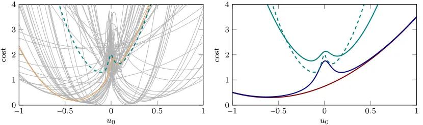
1 from Eq. (8) is already a rational function of fourth order inb0, and shows up quadratically in Eq. (9), the relevant expectations cannot be computed in closed form (Aoki, 1967). For this simple case though, it is possible to compute the optimal dual control by performing the expectation through sampling b, ξ0, ξ1 from the prior. Fig. 1 shows such samples of L(u0) (in gray; one single sample highlighted in orange), and the empirical expectationJ(u0)in dashed green. Each sample is a rational function of even leading order. In contrast to the CE cost, the dual cost is much narrower, leading to more cautious behavior of the dual controller. The average dual cost has its minima not at zero, but to either side of it, reflecting the optimal amount of exploration in this particular belief state.

−1 −0.5 0 0.5 1 0

1 2 3 4

u0

cost

−1 −0.5 0 0.5 1 0

1 2 3 4

u0

cost

Figure 1: Left: Computing the T =2 dual cost for the simple system of Eq. (5). Costs

L(u0)under optimal control onu1 for sampled parameterb(thin gray; one sample highlighted, orange). Expected dual cost J(u0) underu∗1 (dashed green). The optimalu∗

0 lies at the minimum of the dashed green line. Right: Comparison of sampling (dashed green; thin gray: samples) to three approximations: CE (red) and CE with Bayesian exploration bonus (blue). The solid green line is the approximate dual control constructed in Section 4. See also Sec. 6.1 for details.

(however, see Poupart et al., 2006, for a sampling solution to Bayesian reinforcement learning in discrete spaces, including notes on the considerable computational complexity of this approach). The next section describes a tractable analytic approximation that does not involve samples.

4. Approximate Dual Control for Linear Systems

In 1973, Tse et al. (1973) constructed theory and an algorithm (Tse and Bar-Shalom, 1973) for approximate dual (AD) control, based on the series expansion of the cost-to-go. This is related to differential dynamic programming for the control of nonlinear dynamic systems (Mayne, 1966). It separates into three conceptual steps (described in Sec. 4.1–4.3), which together yield what, from a contemporary perspective, amounts to a structured Gaussian approximation to Bayesian RL:

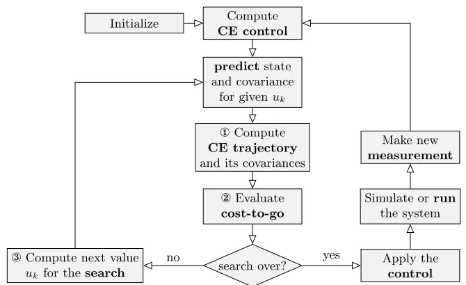
¬ Find an optimal trajectory for the deterministic part of the system under the mean model: thenominal trajectory under certainty equivalent control. For linear systems this is easy (see below), for nonlinear ones it poses a nontrivial, but feasible nonlinear model predictive control problem (Allg¨ower et al., 1999; Diehl et al., 2009). It yields a nominal trajectory, relative to which the following step constructs a tractable quadratic expansion.

Initialize Compute CE control

predictstate and covariance

for givenuk

¬Compute CE trajectory and its covariances

­Evaluate cost-to-go

search over?

®Compute next value

uk for thesearch

Apply the control Simulate orrun

the system Make new measurement

yes no

Figure 2: Flow-chart of the approximate dual control algorithm to show the overall structure. Adapted from Tse and Bar-Shalom (1973). The left cycle is the inner loop, performing the nonlinear optimization.

® In the current time stepk, perform the prediction for an arbitrary control input uk (as opposed to the analytically computed control input for later steps). Optimizeuk numerically by repeated computation of steps¬and ­at varyinguk to minimize the approximate cost.

These three steps will be explained in detail in the subsequent sections. The interplay between the different parts of the algorithm is shown in Figure 2.

The abstract introductory work Tse et al. (1973) is relatively general, but the explicit formulation in Tse and Bar-Shalom (1973) only applies to linear systems. Since both works are difficult to parse for contemporary readers, the following sections thus first provide a short review, before we extend to more modern concepts. In this section, we follow the more transparent case of a linear system from Tse and Bar-Shalom (1973), i.e. φ(x) =x in Eq. (1). For the augmented statez, this still gives a nonlinear system, because θ andx interact multiplicatively

zk+1= ( xk+1 θk+1) = (

A(θk) 0

0 I)zk+ (

B(θk)

0 )uk+ ( ξk

0) =∶f˜(zk, uk). (10) The parameters θ are assumed to be deterministic, but not known to the controller. This uncertainty is captured by the distribution p(θ) representing the lack of knowledge.

4.1 Certainty Equivalent Control Gives a Nominal Reference Trajectory

which decouples θ entirely fromx in Eq. (10), and the optimal control for the finite horizon problem can be computed by dynamic programming (DP) (Aoki, 1967), yielding an optimal linear control law

¯ u∗

j = − (B¯ ⊺¯

Kj+1B¯+Uj) −1 _¯

B⊺[¯

Kj+1A¯x¯j+p¯j+1],

where we have momentarily simplified notation to ¯A=A(θ¯j),B¯=B(θ¯j),∀j, because the ¯θj are constant. The ¯Kj and ¯pj forj=k+1, . . . , T are defined and computed recursively as

¯

Kj =A¯⊺(K¯j+1−K¯j+1B¯(B¯⊺K¯j+1B¯+Uj) −1 _¯

B⊺¯

Kj+1)A¯+Wj K¯T =WT ¯

pj =A¯⊺(p¯j+1−K¯j+1B¯(B¯⊺K¯j+1B¯+Uj) −1 _¯

B⊺ ¯

Kj+1)p¯j+1−Wjrj p¯T = −WTrT,

where r is the reference trajectory to be followed. This CE controller gives the nominal trajectory of inputs ¯uk∶T−1and states ¯xk∶T, from the current timekto the horizonT. The true future trajectory is subject to stochasticity and uncertainty, but the deterministic nominal trajectory ¯x, with its optimal control ¯u∗

and associated nominal cost ¯J∗

k = L(x¯k∶T,u¯ ∗ k∶T) provides a base, relative to which an approximation will be constructed.

4.2 Quadratic Expansion Around the Nominal Defines Cost of Uncertainty

The central idea of AD control is to project the nonlinear objective Jk(uk∶T−1, p(xk)) of Eq. (3) into a quadratic, by locally linearizing around the nominal trajectory x and maintaining a joint Gaussian belief.

To do so, we introduce small perturbations around nominal cost, states, and control: ∆Jj =Jj −J¯j,∆zj =zj −z¯j, and ∆uj =uj −u¯j. These perturbations arise from both the stochasticity of the state and the parameter uncertainty. Note that a change in the state results in a change of the control signal, because the optimal control signal in each step depends on the state. Even though the origin of the uncertainties is different (∆x arises from stochasticity and ∆θ from the lack of knowledge), both can be modeled in a joint probability distribution.

Approximate Gaussian filtering ensures that beliefs over ∆z remain Gaussian:

p(∆zj) = N [( ∆xj ∆θj)

;(∆ˆxj 0 ),(

Σxx_j Σxθ_j Σθx_j Σθθ_j )].

Note that shifting the mean to the nominal trajectory does not change the uncertainty. Note further that the expected perturbation in the parameters is nil. This is because the parameters are assumed to be deterministic and are not affected by any state or input.

Calculating the Gaussian filtering updates is in principle not possible for future measure-ments, since it violates the causality principle (Glad and Ljung, 2000). Nonetheless, it is possible to use theexpected measurements to simulate the effects of the future measurements on the uncertainty, since these effects are deterministic. This is sometimes referred to as preposterior analysis (Raiffa and Schlaifer, 1961).

To second order around the nominal trajectory, the cost is approximated by

Jk(uk∶T−1, p(xk)) =J¯ ∗

where ¯J∗

k is the optimal cost for the nominal system and ∆ ˜Jk is the approximate additional cost from the perturbation:

∆ ˜Jk∶=Exk∶T

⎡⎢ ⎢⎢ ⎢⎣ T ∑ j=k

{(x¯j−rj)⊺Wj∆xj+ 1 2∆x

⊺

jWj∆xj} + T−1

∑ j=k

{u¯⊺

jUj∆uj+ 1 2∆u

⊺

jUj∆uj} ⎤⎥ ⎥⎥ ⎥⎦.

(12) Although the uncertain parameters θdo not show up explicitly in the above equation, this step captures dual effects: The uncertainty of the trajectory ∆x depends on θ via the dynamics. Higher uncertainty overθ at time j−1 causes higher predictive uncertainty over ∆xj (for each j), and thus increases the expectation of the quadratic term ∆x⊺jWj∆xj. Control that decreases uncertainty inθcan lower this approximate cost, modeling the benefit of exploration. For the same reason, Eq. (12) is in fact still not a quadratic function and has no closed form solution. To make it tractable, Tse and Bar-Shalom (1973) make the ansatz that all terms in the expectation of Eq. (12) can be written as gj+p⊺_j∆zj+1/2∆z_j⊺Kj∆zj. This amounts to applying dynamic programming on the perturbed system. Expectations over the cost under Gaussian beliefs on ∆z can then be computed analytically. Because all ∆θ have zero mean, linear terms in these quantities vanish in the expectation. This allows analytic minimization of the approximate optimal cost for each time step

∆ ˜J∗

j(p(xj)) =min ∆uj{(

xj−rj)⊺Wj∆ˆxj∣j+ 1 2∆ˆx

⊺

j∣jWj∆ˆxj∣j+u ⊺

jU∆uj+ 1 2∆u

⊺ jU∆uj

+1

2tr[WjΣ xx j∣j] + E

∆xj+1[

∆ ˜J∗

j+1(y1∶j+1) ∣p(xj)]}, (13) which is feasible given an explicit description of the Gaussian filtering update. It is important to note that, assuming extended Kalman filtering, the update to the mean from expected

future observations yj+1 is nil. This is because we expect to see measurements consistent with the current mean estimate. Nonetheless, the (co-)variance changes depending on the control input uj, which is the dual effect.

Following the dynamic programming equations for the perturbed problem, including the additional cost from uncertainty, the resulting cost amounts to (Tse et al., 1973)

∆ ˜J∗

k(p(xk)) =g˜k+1+p˜⊺k+1∆ˆzk+ 1 2∆ˆz

⊺

kK˜k+1∆ˆzk

+1

2tr

⎧⎪⎪ ⎨⎪⎪ ⎩

WTΣxxT∣T + T−1

∑ j=k

[WjΣxxj∣j+ (Σj+1∣j−Σj+1∣j+1)K˜j+1]

⎫⎪⎪ ⎬⎪⎪ ⎭

(where we have neglected second-order effects of the dynamics). Recalling that ∆ˆz=0 and dropping the constant part, the dual cost can be approximated to be

J_kd=1 2tr

⎧⎪⎪ ⎨⎪⎪ ⎩

WTΣxxT∣T + T−1

∑ j=k

[WjΣxxj∣j+ (Σj+1∣j−Σj+1∣j+1)K˜j+1]

⎫⎪⎪ ⎬⎪⎪

⎭ (=

∆ ˜J∗

k−const)

where the recursive equation

˜

Kj =A˜⊺(K˜j+1−K˜j+1B˜(B⊺Kjxx+1B+Uj) −1 _˜

B⊺˜

is defined for the augmented system (10), with ˜A= _∂z∂ f˜, ˜B= _∂u∂ f˜and ˜Wj=blkdiag(Wj,0). The approximation to the overall cost is then ¯J∗

k +Jkd, which is used in the subsequent optimization procedure.

4.3 Optimization of the Current Control Input Gives Approximate Dual Control

The last step®amounts to the outer loop of the overall algorithm. A gradient-free black-box optimization algorithm is used to find the minimum of the dual cost function. In every step, this algorithm proposes a control input uk for which the dual cost is evaluated.

Depending on uk, approximate filtering is carried out to the horizon. The perturbation control is plugged into Eq. (13) to give an analytic, recursive definition for ˜Kj, and an approximation for the dual costJ_kd, as a function of the current control input uk.

Nonlinear optimization—through repetitions of steps ¬and­ for proposed locations uk—then yields an approximation to the optimal dual control u∗k. Conceptually the simplest part of the algorithm, this outer loop dominates computational cost, because for every locationuk the whole machinery of¬and ­ has to be evaluated.

5. Extension to Contemporary Machine Learning Models

The preceding section reviewed the treatment of dual control in linear dynamical systems from Tse and Bar-Shalom (1973). In this section, we extend the approach to inference on, and dual control of, the dynamics of nonlinear dynamical systems. This extension is guided by the desire to use a number of popular, standard regression frameworks in machine learning: Parametric general least-squares regression, nonparametric Gaussian process regression, and feedforward neural networks (including the base case of logistic regression).

5.1 Parametric Nonlinear Systems

We begin with the generalized linear model mentioned in Eq. (1). The nonlinear features φcan in principle be any function (popular choices include sines and cosines, radial basis functions, sigmoids, polynomials and others), with the caveat that their structure crucially influences the properties of the model. From a modeling perspective, this approach is quite standard for machine learning. However, the dynamical learning setting requires a few adaptations: First, to allow the modeling of higher-order dynamical systems, the original states must to be included. This gives features of the form φ(x)⊺= (_x⊺ _ϕ(_x)⊺)_{, consisting} of the linear representation, augmented by general features ϕ.

The next challenge is that the optimal control for nonlinear dynamical systems cannot be optimized in closed form using dynamic programming, not even for the deterministic nominal system. Instead, we find the nominal reference trajectory using nonlinear model predictive control (Allg¨ower et al., 1999; Diehl et al., 2009). In our case, we begin with dynamic programming on a locally linearized system, then optimize nonlinearly with a numerical method across the trajectory. This adds computational cost, and requires some care to achieve stable optimization performance for specific system setups.

to retain Gaussian beliefs over the states and parameters. Extensions of this approach to more elaborate filtering methods are an interesting direction for future work. This includes relatively standard options like unscented Kalman filtering (Uhlmann, 1995), but also more recent developments in machine learning and probabilistic control, such as analytic moment propagation where the featuresϕallow this (e.g., Deisenroth and Rasmussen, 2011).

The final problem is the generalization of the derivations from the preceding sections to the nonlinear dynamics. We take a relatively simplistic approach, which nevertheless turns out to work well. A linearization gives locally linear dynamics whose structure closely matches Eq. (10):

zk+1= ( ¯

xk+1+∆xk+1 ¯

θk+1+∆θk+1) = (

A(θk) 0 0 I) (

φ(x¯k+∆xk) ¯

θk+∆θk ) + (

B(θk)

0 )uk+ ( ξk

0)

≈ (A(θ¯k) 0 0 I) (

φ(x¯k) ¯

θk ) + (

B(θ¯k)

0 )uk+ ( ξk

0)

+ (A(θ¯k)_∂x∂_kφ(x¯k) _∂θ∂_k(A(θ¯k)φ(x¯k) +B(θ¯k)uk)

0 I ) (

∆xk ∆θk)

.

This essentially amounts to extended Kalman filtering on the augmented state. Using this linearization, the approximation described in Sec. 4 can be applied analogously.

5.2 Nonparametric Gaussian Process Dynamics Models

The above treatment of parametric linear models makes it comparably easy to extend the description from finitely many feature functions to an infinite-dimensional feature space defining a Gaussian process (GP) dynamics model: Assume that the true dynamics function f is a draw from a Gaussian process prior p(f) = GP(f;m,κ¯) with prior mean function m∶Rn_R

n_{, and prior covariance function (kernel) ¯κ∶}

Rn×Rn_R n_×

Rn. This is using

the widely used notion of “multi-output regression” (Rasmussen and Williams, 2006,§ 9.1), i.e. formulating the covariance as

cov(fi(x), fj(x′)) =κ¯ij(x, x′).

To simplify the treatment, we will assume that the covariance factors between inputs and outputs, i.e. ¯κij(x, x′) =Vijκ(x, x′) with a univariate kernel κ∶Rn×Rn_Rand a positive semi-definite matrix V ∈Rn×n of output covariances. By Mercer’s theorem (e.g., K¨onig,

1986; Rasmussen and Williams, 2006), the kernel can be decomposed into a converging series over eigenfunctionsφ(x), as

κ(x, x′) = ∞

∑ `=1

λ`φ`(x)φ∗`(x ′)

, (14)

whereφ`∶Rn_Rare functions that are orthonormal relative to some measure µover R n

(the precise choice of which is irrelevant for the time being), with the property

∫ κ(x, x′)

Precisely in this sense, Gaussian process regression can be written as “infinite-dimensional” Bayesian linear regression. We will use the suggestive, and somewhat abusive notation fk(xk) =LΩkΦ(xk) for this generative model, defined as

f_ki(xk) = T ∑ j=1 Lij ∞ ∑ `=1

Ωj`_kφi(xk) (15)

whereL is a matrix satisfyingLL⊺=

V (e.g., the Cholesky decomposition), and the elements of Ω are draws from the “white” Gaussian process Ωj`<sub>k</sub> ∼ N (0, λ`). Because of Mercer’s theorem above, Eq. (15) exists in µ2 expectation, and is well-defined in this sense. This notation allows writing Eq. (2) as a nonparametric prior with mean ˆθ0 and covariance Σθθ₀ =V ⊗ (ΦΛΦ⊺) _{where Λ is an infinite diagonal matrix with diagonal elements Λ}

``=λ` (the matrix multiplication ΦΛΦ⊺ _{is here defined as in Eq. (15)).}

Using this notation, a tedious but straightforward linear algebra derivation (see Ap-pendix A) shows that the posterior over z⊺= (_x⊺ _θ⊺)_{after a numberk of EKF-linearized} Gaussian observations is a tractable Gaussian process, for which the Gram matrix

G = P + Q + K + F−1_RF−⊺

consists of the parts

P = [P0 0

0 0] Q = (Q⊗I) K =κ(y1∶m,y1∶m) R = (R⊗I)

of appropriate size, depending on the current timek. The multi-step state transition matrix

F = ⎡⎢ ⎢⎢ ⎢⎢ ⎢⎢ ⎢⎢ ⎣

I 0 0 ⋯ 0

A1 I 0 ⋯ 0

A2A1 A2 I ⋯ 0

⋮ ⋱

Am⋯A1 Am⋯A2 ⋯ I

⎤⎥ ⎥⎥ ⎥⎥ ⎥⎥ ⎥⎥ ⎦

with F−1=

⎡⎢ ⎢⎢ ⎢⎢ ⎢⎢ ⎢⎢ ⎣

I 0 0 ⋯ 0

−A1 I 0 ⋯ 0

0 −A2 I ⋯ 0

⋮ ⋱ ⋱ ⋱

0 ⋯ 0 −Am I ⎤⎥ ⎥⎥ ⎥⎥ ⎥⎥ ⎥⎥ ⎦

is needed to account for the effect of the measurement noiseR over time. The A-matrices are the Jacobians ∇xf(x)∣xk.

The posterior mean now evaluates to

[xˆk ˆ

θk] = [ ˆ xk−1

0 ] + [

Φ(xˆk−1)ΛΦ(y1∶k−1)⊺ ΛΦ(y_1∶k−1)⊺ ] G

−1_[Φ(y

1∶k−1)ΛΦ(xˆk−1)⊺ Φ(y1∶k−1)Λ] (16) and the posterior covariance is comprised of

¯

Σxx_k =AkΣxxk A ⊺

k+Q+ΦkΣθxk A ⊺

k+AkΣxθk Φ ⊺

k+ΦkΣθθΦ⊺k (17a) Σxx_k =Σ¯xx_k−1−Σ¯xx_k−1[Σ¯xx_k−1+R]−1Σ¯xx_k−1 (17b) Σxθ_k = Fk,∶Φ(y)Λ− Fk,∶[P + K + Q] G

−1_{Φ(y)Λ (17c)}

Σθx_k = (Σxθ_k )⊺

(17d)

Σθθ_k =Λ−ΛΦ(y)⊺G−1

This formulation, together with the expositions in the preceding sections, defines a nonparametric dual control algorithm for Gaussian process priors. It is important to stress that this posterior is indeed “tractable” in so far as it depends only on a Gram matrix of size nT ×nT, and the posterior over any f(x) can be computed in timeO((nT)3), despite the infinite-dimensional state space.

5.2.1 An Approximation of Constant Cost

In practical control applications, continuously rising inference cost is rarely acceptable. It is thus necessary to project the GP belief onto a finite representation, replacing the infinite sum in Eq. (14) with a finite one, to bound the computational cost of the matrix inversion in Eqs. (16), (17c) and (17e). We do so by projecting into a pre-defined finite basis of functions drawn from the eigen-spectrum of the kernel with respect to the Lebesgue measure. This approach has been recently popular elsewhere in regression (Rahimi and Recht, 2008). For readers unaware of this line of work, here is a short, self-contained introduction:

By Bochner’s theorem (e.g., Stein, 1999; Rasmussen and Williams, 2006), the covariance function k(r) (with r = ∣x−x′∣_{) of a stationary µ}2 _{continuous random process can be} represented as the Fourier transform of a positive finite measure and, if that measure has a densityS(s), as the Fourier dual of S:

κ(r) = ∫ S(s)e2πisrds,

This means that the eigenfunctions of the kernel are trigonometric functions, and stationary covariance functions, like the commonly used square exponential kernel

κ_se(x, x′) =

exp(−(x−x ′)2 2λ2 ), can be approximated by sine and cosine basis functions as

κ(x, x′) ≈ ˜

κ(x, x′) =

√

2 F

F/2 ∑ i=1

sin(ω2i−1∣x−x′∣) +cos(ω2i∣x−x′∣),

where the frequencies ωi of the feature functions is sampled from the power spectrum of the process. An example of such kernel approximation is shown in Fig. 3. With increasing number of features, the approximation can be chosen as closely to the true covariance function as needed, while keeping the number of features in a range that is still feasible within the time constraints of the control algorithm.

5.3 Dual Control of Feedforward Neural Networks

Another extension of the parametric linear models of Section 5.1 is to allow for a nonlinear parametrization of the dynamics function:

f(x;θ) =

F ∑

i

−4 −2 0 2 4 −4

−2 0 2 4

k

e

rnel

app

ximation

−4 −2 0 2 4 −4

−2 0 2 4

−4 −2 0 2 4 −4

−2 0 2 4

posterior

−4 −2 0 2 4 −4

−2 0 2 4

full

k

ernel

prior

−4 −2 0 2 4 0

0.5 1

−4 −2 0 2 4 0

0.5 1

kernel

Figure 3: Prior (left), posterior (middle) and kernel function (right) of both the full kernel function (top row) and the approximate kernel (bottom row). The thick lines represent the mean and the thin lines show two standard deviations. The dashed lines are samples from the shown distributions.

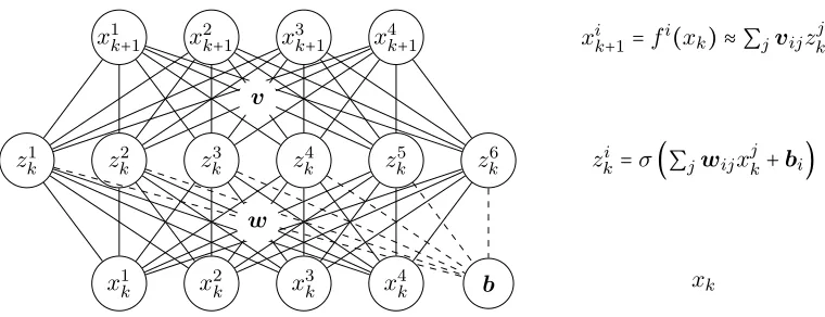
x1_k+1 x2_k+1 x3_k+1 x4_k+1

z_k1 z_k2 z_k3 z_k4 z5_k z_k6

b

x1_k x2_k x3_k x4_k xk

w

z_ki =σ(∑_jwijxj_k+bi)

v

xi_k+1=fi(xk) ≈ ∑jvijz_kj

A particularly interesting example of this structure are multilayer perceptrons. Consider a two-layer network with logistic link function

f(x) = ∑

i

viσ(wix+bi), (18)

where v are the weights from the latent to the output layer,w are the weights from input to hidden units, andbare the biases of the hidden units (see Fig. 4).

Neural networks are used in control quite regularly, see e.g., Nguyen and Widrow (1990). Instead of using backpropagation and stochastic gradient descent as in most applications of neural networks (Rumelhart et al., 1986; Robbins and Monro, 1951), the EKF inference procedure can be used to train the weights as well (Singhal and Wu, 1989). This is possible because the EKF linearization can also be applied for the nonlinear link function, e.g., the logistic function. Speaking in terms of feature functions, not only the weight of each feature but also the shape (steepness) can be inferred. A limiting factor for this inference naturally is the number of data points: the more features and parameters are introduced, the more data points are necessary to learn.

Using the state augmentation z⊺= (_x⊺_v⊺_w⊺)_{, and linearizing w.r.t. all parameters in} each step, the EKF inference on the neural network parameters allows us not only to apply relatively cheap inference on them, but also to use the dual control framework to plan control signals, accounting for the effect of future observations and the subsequent change in the belief. This means the adaptive dual controller described in Sec. 4 can identify those parts of the neural net that are relevant for applying optimal control to the problem at hand. In Sec. 6.3, we show an experiment with these properties.

6. Experiments

A series of experiments on single-episode tasks with continuous state space highlights qualitative differences between the adaptive dual (AD) controller and three other controllers: An oracle controller with access to the true parameters, which provides an unattainable lower bound (LB) on the achievable performance, a certainty equivalent (CE) controller as described in Sec. 4.1, and a controller minimizing the sum of CE cost and the Bayesian exploration bonus (BEB) (see Kolter and Ng, 2009):

`beb=τ[sqrt(diag(Σθθ))] ⊺

[sqrt(diag(Σθθ))]

(τ is a scalar exploration weight). The additional cost term`bebis evaluated for the predicted parameter covariance where the prediction time is chosen according to the order of the system such that the effect of the current control signal shows up in the belief over the parameters. This type of controller is sometimes also called dual control, while being referred to as explicit dual control, where the dual features are obtained by a modified cost function (Filatov and Unbehauen, 2000).

The feature set used for a specific application is part of the prior assumptions for that application. Large uncertainty requires flexible models (which take longer to converge, and require more exploration). Feature selection is important, but since it is independent of the dual control framework itself and a broad topic on its own, it is beyond the scope of this paper. In the following experiments, different feature sets are used both as examples for the flexibility of the framework, but also to model different structural knowledge about the problems at hand.

6.1 On a Simple Scalar System, AD Control Matches Exact Dual Control Well

For the noise-free linear system of Sec. 3.1, (a=1 (known),b=2,p(b) = N (b; 1,10),Q=10−1, R = 0, W = 1, Λ = 1, T = 2), Fig. 1, right, compares the cost functions of the various controllers and the approximately exact sampling solution (which is only available for this very simple setup). All cost functions are shifted by an irrelevant constant. The CE cost is quadratic and indifferent about zero. The BEB (τ =0.1) gives additional structure near zero that encourages learning. While qualitatively similar to the dual cost, its global minimum is almost at the same location as that of CE. The dual control approximates the sampling solution much closer.

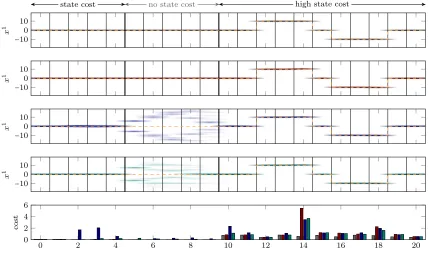
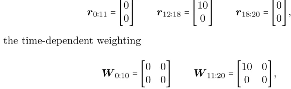
6.2 Faced with Time-Varying State Cost, AD Control Holds Off Exploration Until Suitable

A cart on a rail is a simple example for a dynamical system. Combined with a nonlinearly varying slope, a simple but nonlinear system can be constructed. The dynamics, prior beliefs, and true values for the parameters are chosen to be

xk+1= [ 1 0.4

0 1 ]xk+ [ 0 0 θ1 θ2] [

ϕ1(x1_k) ϕ2(x1_k)] + [

0

1]uk θ∼ N ([ 0 0],[

1 0

0 1]) θtrue= [ 0.8 0.4], where superscripts denote vector elements. The nonlinear functionsϕ are shifted logistic functions of the form

ϕ1(x) = − 1

1+e(x+5) ϕ

2_{(x) =} 1

1+e−(x−5), (19) and disturbance/noise is chosen to be R=Q=10−2I. We use this setup as a testbed for a time-structured exploration problem. The actual system and its dynamics are relatively irrelevant here, as we will focus on a complication caused by the cost function: The reference to be tracked is

r0∶11= [ 0

0] r12∶14= [ 10

0] r15= [ 0

0] r16∶18= [− 10

0 ] r19∶20= [ 0 0]; it is also shown in each plot of Fig. 5 as dashed orange line. The state weighting is time-dependent

W0∶5= [

10 0

0 0] W5∶10= [ 0 0

0 0] W11∶20= [ 100 0

−10 0 10

x

1

0 2 4 6 8 10 12 14 16 18 20

0 2 4 6

cost

−10 0 10

x

1

−10 0 10

x

1

−10 0 10

x

1

state cost no state cost high state cost

Figure 5: Top four: Density estimate for 50 trajectories (first state). From top to bottom: optimal oracle control (gray), certainty equivalent control (red), CE with Bayesian exploration bonus (blue), approximate dual control (green). Reference trajectory in dashed orange. Bottom: The mean cost per time step is shown in the bottom plot, with colors matching the controllers noted above.

and control cost is relatively low: Λ=10−3. The task, thus, is to first keep the cart fixed in the starting position to high precision, for the first 4 time steps. This is followed by a “loose” period between time steps 5 and 10. Then, the cart has to be moved to one side, back to the center, to the other side, and back again, all at high cost. A good exploration strategy in this setting is to act cautiously for the first 5 time steps, then aggressively explore in the “loose” phase, to finally be able to control the motion with high precision.

The inference model is a GP with approximated SE kernel, as described in Sec. 5.2.1. We use 30 alternating sine and cosine features that are distributed according to the power spectrum of the full SE kernel. Since the true nonlinearity of Eq. (19) is not of this form, the approximation is out of model and the lower bound controller only represents a perfectly learned, but still not exact, model.

has no way of knowing about the “loose” phase ahead. Of course, this strategy incurs a higher cost initially. The dual controller (bottom) efficiently holds off exploration until it reaches the “loose” phase, where it explores aggressively.

6.3 AD Control Distinguishes Necessary and Unnecessary Parameter Exploration

The system including nonlinearities for this experiment is the same as before, although with noise parameters R =Q=10−3I. The reference trajectory and state weighting are much simpler, though:

r0∶11= [ 0

0] r12∶18= [ 10

0] r18∶20= [ 0 0], with the time-dependent weighting

W0∶10= [ 0 0

0 0] W11∶20= [ 10 0

0 0],

allowing for identification in the beginning, while penalizing deviations of the first state in later time steps.

Important to note here is that the reference trajectory only passes areas of the state space whereϕ1 is strong, and ϕ2 is negligible. Good exploration thus will ignore θ2, but this can only be found through reasoning about future trajectories.

In this experiment, the learned model is of the neural network form described in Sec. 5.3. We use 4 logistic features (see Eq. (18)) with two free parameters each (wi and vi) and equally spaced bi between−5 and 5, the locations of the true nonlinear features. This means it is possible to learn the perfect model in this case.

Fig. 6 shows a density estimated from 50 state trajectories for the four different controllers. Because of symmetry in the cost function and feature functions, BEB (with τ =1) cannot “decide” between the relevantθ1 and the irrelevantθ2, choosing the exploration direction stochastically. It thus sometimes reduces the uncertainty on θ2, which does not help the subsequent control. The AD controller ignores θ2 completely and only identifiesθ1 in early phases, leading to good control performance.

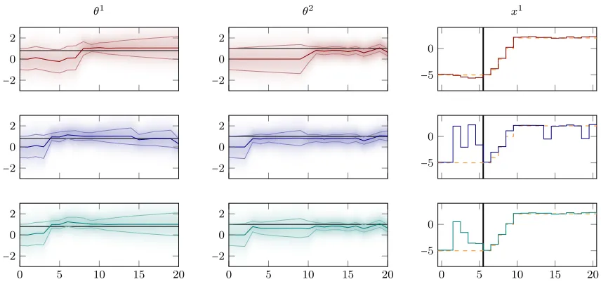
6.4 AD Control Maintains Only Useful Knowledge

The last experiment is again similar to Sec. 6.2, but uses a different set of nonlinear functions, namely shifted Gaussian functions (a.k.a. radial basis functions)

ϕ1(x) =e−(x−2)

2

2 ϕ2(x) =e− (x+2)2

2 θ_true= [1.0

0.8].

−10 0 10

x

1

−10 0 10

x

1

−10 0 10

x

1

−10 0 10

x

1

0 2 4 6 8 10 12 14 16 18 20

0 0.2 0.4 0.6 0.8

cost

no state cost state cost

Figure 6: Top four: Density estimate for 50 trajectories (second state). From top to bottom: optimal oracle control (gray), certainty equivalent control (red), CE with Bayesian exploration bonus (blue), approximate dual control (green). Reference trajectory in dashed orange. Bottom: The mean cost per time step is shown in the bottom plot, with colors matching the controllers noted above.

The reference to be tracked passes through both nonlinear features but then stays at one of them:

r0∶6= [−5

0] r7= [− 4

0] r8= [− 2

0] r9= [ 0

0] r10∶20= [ 2 0].

The cost structure is

W0∶5= [

0 0

0 0] W6∶20= [ 10 0

0 0],

−2 0 2

θ1

−2 0 2

θ2

−5 0

x1

−2 0 2

−2 0 2

0 5 10 15 20

−2 0 2

0 5 10 15 20

−5 0 −5 0

0 5 10 15 20

−2 0 2

Figure 7: Parameter knowledge (left, middle) and state trajectory (right) for different controllers. From top to bottom: certainty equivalent control (red), CE with Bayesian exploration bonus (blue), approximate dual control (green). The true parameters are the black lines.

Exp. 6.1 Exp. 6.2 Exp. 6.3 Exp. 6.4 mean std mean std mean std mean std

Oracle 0.67 0.23 1.75 0.33 7.15 3.85 0.66 0.51 CE 0.84 0.73 2.49 0.74 15.72 5.20 1.76 0.90 CE-BEB 0.99 0.92 2.64 0.37 20.88 6.74 84.91 6.77 AD 0.77 0.43 1.96 0.34 14.33 5.40 1.62 0.56

Table 1: Average and standard deviation of costs in the experiments for 50 runs.

6.5 Quantitative Comparison

The above experiments aim to emphasize qualitative strengths of AD control over simpler approximations. It is desirable for a controllers to deal with flexible models of many parameters, many of which will invariably be superfluous. For reference, Table 6.5 also shows quantitative results: Averages and standard deviations of the cost, from the 50 runs for each controller. The AD controller shows good performance overall; interestingly, it also has low variance. CE and BEB were more prone to instabilities.

7. Conclusion

it in the language of reinforcement learning, and extended it to apply to contemporary inference methods from machine learning, including approximate Gaussian process regression and multi-layer networks. The result is a tractable approximation that captures notions of structured exploration, like the value of waiting for future exploration opportunities, and distinguishing relevant from irrelevant model parameters.

Appendix A. Nonparametric EKF Form

The standard Kalman filter (KF) can be found in many textbooks (e.g., S¨arkk¨a, 2013) and therefore will not be restated here. Starting from the standard equations, we derive a general multi-step formulation of the classic KF with

p(zk) = N (zk, mk, Pk).

From there, state augmentation with an infinite-dimensional weight vector gives the expected result.

A.1 Derivation of the Multi-Step KF Formulation

Assuming that the result of the KF and the Gaussian process framework should be identical under certain circumstances, we wish to transform the KF to a formulation with full Gram matrix. Therefore, the prediction and update step have to be combined to

P1= (A0P0A⊺0+Q) − (A0P0A⊺0+Q)H ⊺

S₁−1H(A0P0A⊺0+Q) ⊺

S1=H(A0P0A⊺0+Q)H ⊺

+R,

which is pretty straightforward. We’re adopting a standard notation, where Pk is the covariance at time step k, Ak is the Jacobian, Q is the drift and R is the measurement covariance. The same can be done for the second time step, but it is beneficial introducing a compact notation for the predictive covariance first

(A1P1A⊺1+Q)

= (A1[(A0P0A⊺0+Q) − (A0P0A⊺0+Q)H ⊺

S₁−1H(A0P0A⊺0+Q) ⊺

]A⊺ 1+Q)

=A1(A0P0A⊺0+Q)A ⊺ 1+Q

´¹¹¹¹¹¹¹¹¹¹¹¹¹¹¹¹¹¹¹¹¹¹¹¹¹¹¹¹¹¹¹¹¹¹¹¹¹¹¹¹¹¹¹¹¹¹¹¹¹¹¹¹¹¹¹¹¹¹¹¹¹¹¹¹¹¹¹¹¹¹¹¹¹¹¹¹¹¸¹¹¹¹¹¹¹¹¹¹¹¹¹¹¹¹¹¹¹¹¹¹¹¹¹¹¹¹¹¹¹¹¹¹¹¹¹¹¹¹¹¹¹¹¹¹¹¹¹¹¹¹¹¹¹¹¹¹¹¹¹¹¹¹¹¹¹¹¹¹¹¹¹¹¹¹¹¶

∶=g11

−A1(A0P0A⊺0+Q)

´¹¹¹¹¹¹¹¹¹¹¹¹¹¹¹¹¹¹¹¹¹¹¹¹¹¹¹¹¹¹¹¹¹¹¹¹¹¹¹¹¹¹¹¹¹¹¹¹¸¹¹¹¹¹¹¹¹¹¹¹¹¹¹¹¹¹¹¹¹¹¹¹¹¹¹¹¹¹¹¹¹¹¹¹¹¹¹¹¹¹¹¹¹¹¹¹¹¹¶

∶=g10

H⊺( S1

¯

∶=g00

)−1_H(A

0P0A⊺0+Q)A ⊺ 1

´¹¹¹¹¹¹¹¹¹¹¹¹¹¹¹¹¹¹¹¹¹¹¹¹¹¹¹¹¹¹¹¹¹¹¹¹¹¹¹¹¹¹¹¹¹¹¹¹¹¸¹¹¹¹¹¹¹¹¹¹¹¹¹¹¹¹¹¹¹¹¹¹¹¹¹¹¹¹¹¹¹¹¹¹¹¹¹¹¹¹¹¹¹¹¹¹¹¹¹¶

∶=g01

=g11−g10H⊺g00−1Hg01. Using the compact notation and definingS2 analogously to S1, we can write the two-step update as

P2= (g11−g10H⊺S1−1Hg01) − (g11−g10H⊺S1−1Hg01)H⊺S2−1H(g11−g10H⊺S1−1Hg01)

P2 =g11−g10H⊺S1−1Hg01−g11H⊺S2−1Hg11−g10H⊺S1−1Hg01H⊺S2−1Hg10H⊺S−11 Hg01

+g11H⊺S2−1Hg10H⊺S1−1Hg01+g10H⊺S1−1Hg01H⊺S2−1Hg11

P2=g11− [g10H⊺ g11H⊺] [

S₁−1+S₁−1Hg01H⊺S2−1Hg10H⊺S1−1 −S1−1Hg01H⊺S2−1

−S₂−1Hg10H⊺S1−1 S2−1 ]

´¹¹¹¹¹¹¹¹¹¹¹¹¹¹¹¹¹¹¹¹¹¹¹¹¹¹¹¹¹¹¹¹¹¹¹¹¹¹¹¹¹¹¹¹¹¹¹¹¹¹¹¹¹¹¹¹¹¹¹¹¹¹¹¹¹¹¹¹¹¹¹¹¹¹¹¹¹¹¹¹¹¹¹¹¹¹¹¹¹¹¹¹¹¹¹¹¹¹¹¹¹¹¹¹¹¹¹¹¹¹¹¹¹¹¹¹¹¹¹¹¹¹¹¹¹¹¹¹¹¹¹¹¹¹¹¹¹¹¹¹¹¹¹¹¹¹¹¹¹¹¹¹¹¹¹¹¹¹¹¹¹¹¹¹¹¹¹¹¹¹¹¹¹¹¹¹¹¹¹¹¹¹¹¹¹¹¹¹¹¹¹¹¹¹¸¹¹¹¹¹¹¹¹¹¹¹¹¹¹¹¹¹¹¹¹¹¹¹¹¹¹¹¹¹¹¹¹¹¹¹¹¹¹¹¹¹¹¹¹¹¹¹¹¹¹¹¹¹¹¹¹¹¹¹¹¹¹¹¹¹¹¹¹¹¹¹¹¹¹¹¹¹¹¹¹¹¹¹¹¹¹¹¹¹¹¹¹¹¹¹¹¹¹¹¹¹¹¹¹¹¹¹¹¹¹¹¹¹¹¹¹¹¹¹¹¹¹¹¹¹¹¹¹¹¹¹¹¹¹¹¹¹¹¹¹¹¹¹¹¹¹¹¹¹¹¹¹¹¹¹¹¹¹¹¹¹¹¹¹¹¹¹¹¹¹¹¹¹¹¹¹¹¹¹¹¹¹¹¹¹¹¹¹¹¹¹¹¹¹¶

∶=G−1

[Hg01 Hg11].

Application of Schur’s lemma gives

G= [Hg00H

⊺+_{R Hg} 01H⊺ Hg10H⊺ Hg11H⊺+R]

Assuming full state measurement (H =I) for compactness of notation, the two-step update is

P2 =g11− [g10⊺ g ⊺ 11] [

g00+R g01 g10 g11+R]

−1

[g01 g11]

=A1(A0P0A⊺0+Q)A ⊺

1+Q− [A1(A0P0A⊺0+Q) (A1(A0P0A⊺0+Q)A ⊺ 1+Q)]

⋅ [(A0P0A⊺0+Q) +R (A0P0A⊺0+Q)A ⊺ 1 A1(A0P0A⊺0+Q) (A1(A0P0A⊺0+Q)A

⊺

1+Q) +R] −1

[ (A0P0A⊺0+Q)A ⊺ 1

(A1(A0P0A⊺0+Q)A ⊺ 1+Q)]

,

(20)

which already looks similar to GP inference. We can now generalize this two-step result to the general form by building the Gram matrix according to

G= FPF⊺+ FQF⊺+ R ,

where the individual parts are

P = [P0 0

0 0] Q = (Q⊗I) R = (R⊗I)

of appropriate size, depending on the current timek. The multi-step state transition matrix

F = ⎡⎢ ⎢⎢ ⎢⎢ ⎢⎢ ⎢⎢ ⎣

I 0 0 ⋯ 0

A1 I 0 ⋯ 0

A2A1 A2 I ⋯ 0

⋮ ⋱

Am⋯A1 Am⋯A2 ⋯ I

⎤⎥ ⎥⎥ ⎥⎥ ⎥⎥ ⎥⎥ ⎦

, with F−1=

⎡⎢ ⎢⎢ ⎢⎢ ⎢⎢ ⎢⎢ ⎣

I 0 0 ⋯ 0

−A1 I 0 ⋯ 0

0 −A2 I ⋯ 0

⋮ ⋱ ⋱ ⋱

0 ⋯ 0 −Am I ⎤⎥ ⎥⎥ ⎥⎥ ⎥⎥ ⎥⎥ ⎦ ,

is also needed so shift the initial covariance and drift covariances through time. Put together, this results in

Pk= Fk,∶(P + Q)F ⊺

k,∶− Fk,∶(P + Q)F(FPF ⊺

+ FQF⊺

+ R)−1_F⊺

(P + Q)F∶,k.

A more compact notation can be achieved by using F−1 to obtain Pk= Fk,∶(P + Q)F

⊺

k,∶− Fk,∶(P + Q)(P + Q + F

−1_RF−⊺)−1(P + Q)F

∶,k. (21)

Calculating the mean prediction is done analogously:

mk= Fk,0m0+ Fk,∶(P + Q)(P + Q + F

−1_RF−⊺)−1

y.

A.2 Augmenting the State

Instead of tracking only the state covariance, in the GP setting also the dynamics function has to be inferred. The system equations of the nonlinear system are now

where f ∼ GP(0, k). The inference in this model can be done through the EKF with augmented state. We adopt the weight-space view with f = Φ⊺_{w (see Rasmussen and} Williams, 2006) to augment the state with the infinite-dimensional weight vector w:

z= (x

w) Σ= (

P Σxw

Σwx Σww) JA= ( ∂f¯ ∂x

∂f¯ ∂w 0 I ) = (

A Φ 0 I),

where, in (20), the original x is replaced by the augmentedz,P by Σ and A by JA. Choosing H = [I 0]so that H recovers the original states from the augmented state vector, we obtain, after calculations similar to those above, a Gram matrix with additional terms including feature functions and the prior on them:

G⋆

=G+ ( Φ0Σ

ww

0 Φ⊺0 Φ0Σww0 (Φ⊺0A ⊺ 1+Φ

⊺ 1)

(A1Φ0+Φ1)Σww₀ Φ⊺

0 (A1Φ0+Φ1)Σww0 (Φ⊺0A ⊺ 1+Φ

⊺ 1))

.

At this point it is important to note that the infinite inner product ΦkΣww0 Φ⊺k corresponds to an evaluation of the kernel

Φ(x)Σww₀ Φ(x)⊺

= ∑φi(x)Σww0,ijφj(x′) =κ(x, x′). This means we can write the Gram matrix as

G⋆=

G+ ( κ00 κ00A ⊺ 1+κ01

A1κ00+κ10 A1κ00A⊺1+κ10A⊺1+A1κ01+κ11) ,

where we have written κ⋅⋅ forκ(⋅,⋅) to save space. In total, the Gram matrix is then G⋆

= FPF⊺

+ FQF⊺

+ FKF⊺

+ R,

with K =κ(y_1∶m,y_1∶m). Since inference is more compact and numerically stable if we absorb

F into the Gram matrix as in Eq. (21), we define

G = P + Q + K + F−1_RF−⊺ .

Inference is done according to

Pk= Fk,∶(P + Q + K)F ⊺

k,∶− Fk,∶(P + Q + K)G

−1_{(P + Q + K)F} ∶,k

Σwx_k = (Σxw_k )⊺

= Fk,∶Φ(y)Σww0 − Fk,∶(P + K + Q) G

−1_Φ(y)Σww 0 Σww_k =Σww₀ −Σww₀ Φ(y)⊺G−1

Φ(y)Σww₀ for the covariance and

mk= Fk,0m0+ Fk,∶(P + Q + K)G −1_y

¯

wk=w¯0+Σww0 Φ(y) ⊺G−1

y

Appendix B. Gradients and Hessians of Dynamics Functions

B.1 Neural Network Basis Functions

The neural network dynamics function is

f(x) =

F ∑ i=1

viσ(wi(x−bi)), σ(a) = 1 1+e−a, with the well-known derivatives of the logistic

∂

∂aσ(a) =σ(a)(1−σ(a)),

∂2

∂a2σ(a) =σ(a) (1−σ(a) (3−2σ(a))). The gradient of f(x) can easily found to be

∇f(x) =

⎡⎢ ⎢⎢ ⎢⎢ ⎢⎢ ⎢⎢ ⎢⎢ ⎢⎢ ⎢⎣ ∑F

i=1viwiσ(wi(x−bi))(1−σ(wi(x−bi)))

σ(w1(x−b1))

⋮

σ(wF(x−bF))

v1(x−b1)σ(w1(x−b1))(1−σ(w1(x−b1)))

⋮

vF(x−bF)σ(wF(x−bF))(1−σ(wF(x−bF))) ⎤⎥ ⎥⎥ ⎥⎥ ⎥⎥ ⎥⎥ ⎥⎥ ⎥⎥ ⎥⎦ .

The Hessian, written in parts, using ai=wix+bi, is: ∇2

xf(x) = F ∑ i=1

viw2iσ(ai)(1−σ(ai)(3−2σ(ai))) ∇x∇vif(x) =wiσ(ai)(1−σ(ai))

∇x∇wif(x) =viσ(ai)(1−σ(ai)) + (x−bi)wiviσ(ai)(1−σ(ai))((1−2σ(ai))

∇vi∇vif(x) =0

∇vi∇wif(x) = (x−bi)σ(ai)(1−σ(ai))

∇wi∇wif(x) =vi(x−bi)

2_σ(a

i)(1−σ(ai)(3−2σ(ai))). B.2 Fourier Basis Functions

The Fourier approximation to the dynamics function has the form

f(x) =

√

2 F

F/2 ∑ i=1

v2i−1sin(ω2i−1x) +v2icos(ω2ix). The gradient of f(x) can easily verified to be

∇f(x) =

⎡⎢ ⎢⎢ ⎢⎢ ⎢⎢ ⎢⎢ ⎢⎢ ⎢⎢ ⎢⎢ ⎢⎣ √ 2 F ∑

F/2

i=1v2i−1ω2i−1√cos(ω2i−1x) −v2iω2isin(ω2ix) 2

F sin(ω1x) √

2

F cos(ω2x) ⋮ √

2

F sin(ωF−1x) √

2

F cos(ωFx)

The Hessian, written in parts, using c=√2/_{F for normalization, is:}

∇2

xf(x) =c

F/2 ∑ i=1

−v2i−1ω22i−1sin(ω2i−1x) −v2iω22icos(ω2ix)

∇x∇vif(x) =

⎧⎪⎪ ⎨⎪⎪ ⎩

cωicos(ωix) i odd −cωisin(ωix) i even ∇vi∇vif(x) =0.

B.3 Radial Basis Functions

With radial basis function features, the dynamics function is

f(x) =

F ∑ i=1

viexp(−(

x−ci)2 2λ2 ). The gradient of f(x) is

∇f(x) =

⎡⎢ ⎢⎢ ⎢⎢ ⎢⎢ ⎢⎢ ⎢⎣

∑F

i=1viexp(−(x−ci)

2

2λ2 )

(ci−x) 2λ2

exp(−(x−c1)2 2λ2 ) ⋮

exp(−(x−cF)2 2λ2 )

⎤⎥ ⎥⎥ ⎥⎥ ⎥⎥ ⎥⎥ ⎥⎦

.

The Hessian, written in parts, is:

∇2 xf(x) =

F ∑ i=1

viexp(−(

x−ci)2 2λ2 ) [(

ci−x 2λ2 )

2

− 1

λ2]

∇x∇vif(x) =exp(−(

x−ci)2 2λ2 )

ci−x 2λ2

∇vi∇vif(x) =0

References

F. Allg¨ower, T.A. Badgwell, J.S. Qin, J.B. Rawlings, and S.J. Wright. Nonlinear predictive control and moving horizon estimationan introductory overview. In Advances in Control, pages 391–449. Springer, 1999.

M. Aoki. Optimization of Stochastic Systems. Academic Press, New York - London, 1967.

J.-Y. Audibert, R. Munos, and C. Szepesv´ari. Exploration-exploitation tradeoff using variance estimates in multi-armed bandits. Theoretical Computer Science, 410(19):1876–1902, 2009.

Y. Bar-Shalom and E. Tse. Dual effect, certainty equivalence, and separation in stochastic control. IEEE Transactions on Automatic Control, 19(5):494–500, 1974.

Y. Bar-Shalom and E. Tse. Caution, probing, and the value of information in the control of uncertain systems. Annals of Economic and Social Measurement, 5(3):323–337, 1976.

R.E. Bellman. Adaptive Control Processes: A Guided Tour. Princeton University Press, 1961.

D.P. Bertsekas. Dynamic Programming and Optimal Control. Athena Scientific, 3rd edition, 2005.

O. Chapelle and L. Li. An Empirical Evaluation of Thompson Sampling. In Advances in Neural Information Processing Systems (NIPS), pages 2249–2257, 2011.

R. Dearden, N. Friedman, and D. Andre. Model based Bayesian exploration. In Uncertainty in Artificial Intelligence (UAI), volume 15, pages 150–159, 1999.

M.P. Deisenroth and C.E. Rasmussen. PILCO: A Model-Based and Data-Efficient Approach to Policy Search. In International Conference on Machine Learning (ICML), 2011.

M. Diehl, H.J. Ferreau, and N. Haverbeke. Efficient numerical methods for nonlinear MPC and moving horizon estimation. In Nonlinear Model Predictive Control, volume 384, pages 391–417. Springer, 2009.

S.E. Dreyfus. Some types of optimal control of stochastic systems. Journal of the Society for Industrial & Applied Mathematics, Series A: Control, 2(1):120–134, 1964.

M.O.G. Duff. Optimal Learning: Computational procedures for Bayes-adaptive Markov decision processes. PhD thesis, University of Massachusetts, Amherst, 2002.

A.A. Feldbaum. Dual Control Theory I-IV. Avtomatika i Telemekhanika, 21(9), 21(11), 22(1), 22(2), 1960–1961.

N.M. Filatov and H. Unbehauen. Survey of adaptive dual control methods.IEEE Proceedings on Control Theory and Applications, 147(1):118–128, 2000.

N.M. Filatov and H. Unbehauen. Adaptive Dual Control. Springer Verlag, Berlin, 2004.

T. Glad and L. Ljung. Control theory: Multivariable and Nonlinear Methods. Taylor and Francis, New York, London, 2000.

P. Hennig. Optimal Reinforcement Learning for Gaussian Systems. In Advances in Neural Information Processing Systems (NIPS), 2011.

O.L.R. Jacobs and J.W. Patchell. Caution and probing in stochastic control. International Journal of Control, 16(1):189–199, 1972.

J.Z. Kolter and A.Y. Ng. Near-Bayesian exploration in polynomial time. InInternational Conference on Machine Learning (ICML), 2009.

H. K¨onig. Eigenvalue Distribution of Compact Operators. Birkh¨auser, 1986.

W.G. Macready and D.H. Wolpert. Bandit problems and the exploration/exploitation tradeoff. IEEE Transactions on Evolutionary Computation, 2(1):2–22, 1998.

D.Q. Mayne. A second-order gradient method for determining optimal trajectories of non-linear discrete-time systems. International Journal of Control, 3(1):85–95, 1966.

D.H. Nguyen and B. Widrow. Neural networks for self-learning control systems. IEEE Control Systems Magazine, 10(3):18–23, 1990.

P. Poupart, N. Vlassis, J. Hoey, and K. Regan. An analytic solution to discrete Bayesian reinforcement learning. In International Conference on Machine Learning (ICML), 2006.

A. Rahimi and B. Recht. Random features for large-scale kernel machines. InAdvances in Neural Information Processing Systems (NIPS), pages 1177–1184, 2008.

H. Raiffa and R. Schlaifer.Applied statistical decision theory. Studies in managerial economics. Harvard University, Boston, 1961.

C.E. Rasmussen and C.K.I. Williams. Gaussian Processes for Machine Learning. MIT, 2006.

H. Robbins and S. Monro. A stochastic approximation method. The Annals of Mathematical Statistics, 22(3):400–407, Sep. 1951.

D.E. Rumelhart, G.E. Hinton, and R.J. Williams. Learning representations by back-propagating errors. Nature, 323(6088):533–536, 1986.

S. S¨arkk¨a. Bayesian filtering and smoothing. Cambridge University Press, 2013.

S. Singhal and L. Wu. Training multilayer perceptrons with the extended kalman algorithm. In Advances in Neural Information Processing Systems (NIPS), pages 133–140, 1989.

N. Srinivas, A. Krause, S. Kakade, and M. Seeger. Gaussian Process Optimization in the Bandit Setting: No Regret and Experimental Design. In International Conference on Machine Learning (ICML), 2010.

M.L. Stein. Interpolation of spatial data: some theory for Kriging. Springer Verlag, 1999.

J. Sternby. A simple dual control problem with an analytical solution. IEEE Transactions on Automatic Control, 21(6):840–844, 1976.

W.R. Thompson. On the Likelihood that one unknown probability exceeds another in view of two samples. Biometrika, 25:275–294, 1933.

E. Tse, Y. Bar-Shalom, and L. Meier III. Wide-sense adaptive dual control for nonlinear stochastic systems. IEEE Transactions on Automatic Control, 18(2):98–108, 1973.

J. Uhlmann. Dynamic Map Building and Localization: New Theoretical Foundations. PhD thesis, University of Oxford, 1995.