A Study of the Classification of Low-Dimensional Data with Supervised Manifold Learning

(1)

A Study of the Classification of Low-Dimensional Data with

Supervised Manifold Learning

Elif Vural∗ [email protected]

Department of Electrical and Electronics Engineering Middle East Technical University

Ankara, 06800, Turkey

Christine Guillemot [email protected] Centre de Recherche INRIA Bretagne Atlantique

Campus Universitaire de Beaulieu 35042 Rennes, France

Editor:Gert Lanckriet

Abstract

Supervised manifold learning methods learn data representations by preserving the geomet-ric structure of data while enhancing the separation between data samples from different classes. In this work, we propose a theoretical study of supervised manifold learning for classification. We consider nonlinear dimensionality reduction algorithms that yield linearly separable embeddings of training data and present generalization bounds for this type of algorithms. A necessary condition for satisfactory generalization performance is that the embedding allow the construction of a sufficiently regular interpolation function in relation with the separation margin of the embedding. We show that for supervised embeddings satisfying this condition, the classification error decays at an exponential rate with the number of training samples. Finally, we examine the separability of supervised nonlinear embeddings that aim to preserve the low-dimensional geometric structure of data based on graph representations. The proposed analysis is supported by experiments on several real data sets.

Keywords: Manifold learning, dimensionality reduction, classification, out-of-sample extensions, RBF interpolation

1. Introduction

In many data analysis problems, data samples have an intrinsically low-dimensional struc-ture although they reside in a high-dimensional ambient space. The learning of low-dimensional structures in collections of data has been a well studied topic of the last two decades (Tenenbaum et al., 2000), (Roweis and Saul, 2000), (Belkin and Niyogi, 2003), (He and Niyogi, 2004), (Donoho and Grimes, 2003), (Zhang and Zha, 2005). Following these works, many classification methods have been proposed in the recent years to apply such manifold learning techniques to learn classifiers that are adapted to the geometric struc-ture of low-dimensional data (Hua et al., 2012), (Yang et al., 2011), (Zhang et al., 2012), (Sugiyama, 2007), (Raducanu and Dornaika, 2012). The common approach in such works

∗. Most part of the work was performed while the first author was at INRIA.

(2)

is to learn a data representation that enhances the between-class separation while preserv-ing the intrinsic low-dimensional structure of data. While many efforts have focused on the practical aspects of learning such supervised embeddings for training data, the gen-eralization performance of these methods as supervised classification algorithms has not been investigated much yet. In this work, we aim to study nonlinear supervised dimension-ality reduction methods and present performance bounds based on the properties of the embedding and the interpolation function used for generalizing the embedding.

Several supervised manifold learning methods extend the Laplacian eigenmaps algo-rithm (Belkin and Niyogi, 2003), or its linear variant LPP (He and Niyogi, 2004) to the classification problem. The algorithms proposed by Hua et al. (2012), Yang et al. (2011), Zhang et al. (2012) provide a supervised extension of the LPP algorithm and learn a linear projection that preserves the proximity of neighboring samples from the same class, while increasing the distance between nearby samples from different classes. The method by Sugiyama (2007) proposes an adaptation of the Fisher metric for linear manifold learning, which is in fact shown to be equivalent to the above methods by Yang et al. (2011), Zhang et al. (2012). In (Li et al., 2013), (Cui and Fan, 2012), (Wang and Chen, 2009), some other similar Fisher-based linear manifold learning methods are proposed. In (Raducanu and Dornaika, 2012) a method relying on a similar formulation as in (Hua et al., 2012), (Yang et al., 2011), (Zhang et al., 2012) is presented, which, however, learns a nonlinear embed-ding. The main advantage of linear dimensionality reduction methods over nonlinear ones is that the generalization of the learnt embedding to novel (initially unavailable) samples is straightforward. However, nonlinear manifold learning algorithms are more flexible as the possible data representations they can learn belong to a wider family of functions, e.g., one can always find a nonlinear embedding to make training samples from different classes linearly separable. On the other hand, when a nonlinear embedding is used, one must also determine a suitable interpolation function to generalize the embedding to new samples, and the choice of the interpolator is critical for the classification performance.

(3)

ex-amine the rates of convergence of supervised manifold learning algorithms that satisfy these conditions.

In Section 2, we consider arbitrary supervised manifold learning algorithms that compute a linearly separable embedding of training samples. We study the generalization capability of such algorithms for two types of out-of-sample interpolation functions. We first consider arbitrary interpolation functions that are Lipschitz-continuous on the support of each class, and then focus on out-of-sample extensions with radial basis function (RBF) kernels, which is a popular family of interpolation functions. For both types of interpolators, we derive conditions that must be satisfied by the embedding of the training samples and the regu-larity of the interpolation function that generalizes the embedding to test samples, when a nearest neighbor or linear classifier is used in the low-dimensional domain of embedding. These conditions enforce the Lipschitz constant of the interpolator to be sufficiently small, in comparison with the separation margin between training samples from different classes in the low-dimensional domain of embedding. The practical value of these results resides in their implications about what must really be taken into account when designing a su-pervised dimensionality reduction algorithm: Achieving a good separation margin does not suffice by itself; the geometric structure must also be preserved so as to ensure that a suffi-ciently regular interpolator can be found to generalize the embedding to the whole ambient space. We then particularly consider Gaussian RBF kernels and show the existence of an optimal value for the kernel scale by studying the condition in our main result that links the separation with the Lipschitz constant of the kernel.

Our results in Section 2 also provide bounds on the rate of convergence of the classifi-cation error of supervised embeddings. We show that the misclassificlassifi-cation error probability decays at an exponential rate with the number of samples, provided that the interpolation function is sufficiently regular with respect to the separation margin of the embedding. These convergence rates are higher than those reported in previous results on RBF net-works (Niyogi and Girosi, 1996), (Lin et al., 2014), (Hern´andez-Aguirre et al., 2002), and regularized least-squares regression algorithms (Caponnetto and De Vito, 2007), (Steinwart et al., 2009). The essential difference between our results and such previous works is that those assume a general setting and do not focus on a particular data model, whereas our results are rather relevant to settings where the support of each class admits some certain structure, so as to allow the existence of an interpolator that is sufficiently regular on the support of each class. Moreover, in contrast with these previous works, our bounds are independent of the ambient space dimension and vary only with the intrinsic dimensions of the class supports as they characterize the error in terms of the covering numbers of the supports.

(4)

class and rapidly across different classes. We study the conditions for the linear separability of these embeddings and characterize their separation margin in terms of some graph and algorithm parameters.

In Section 4, we evaluate our results with experiments on several real data sets. We study the implications of the condition derived in Section 2 on the separability margin - interpolator regularity tradeoff. The experimental comparison of several supervised di-mensionality reduction algorithms shows that this compromise between the separation and interpolator regularity can indeed be related to the practical classification performance of a supervised manifold learning algorithm. This suggests that, one can possibly improve the accuracy of supervised dimensionality reduction algorithms by considering more carefully the generalization capability of the embedding during the learning. We then study the vari-ation of the classificvari-ation performance with parameters such as the sample size, the RBF kernel scale, and the dimension of the embedding, in view of the generalization bounds presented in Section 2. Finally, we conclude in Section 5.

2. Performance Bounds for Supervised Manifold Learning Methods

2.1 Notation and Problem Formulation

Consider a setting withM data classes where the samples of each classm∈ {1, . . . , M}are drawn from a probability measure νm in a Hilbert space H such that νm has a bounded

support Mm ⊂ H. Let X = {xi}Ni=1 ⊂ H be a set of N training samples such that each xi is drawn from one of the probability measures νm, and the samples drawn from

each νm are independent and identically distributed. We denote the class label of xi by

Ci∈ {1,2, . . . , M}.

LetY ={yi}N_i₌₁⊂Rdbe ad-dimensional embedding ofX, where eachyi corresponds to

xi. We consider supervised embeddings such thatY is linearly separable. Linear separability

is defined as follows:

Definition 1 The data representation Y is linearly separable with a margin of γ > 0, if

for any two classes k, l ∈ {1,2, . . . , M}, there exists a separating hyperplane defined by

ωkl∈Rd, kωklk= 1 and bkl∈R such that

ωT_klyi+bkl≥γ/2 if Ci =k

ωT_klyi+bkl≤ −γ/2 if Ci =l.

(1)

The above definition of separability implies the following. For any given class m, there exists a set of hyperplanes {ωmk}k6=m ⊂ Rd, kωmkk = 1, and a set of real

num-bers {bmk}k6=m ⊂ R that separate class m from other classes, such that for all yi of class

Ci=m

ω_mkT yi+bmk> γ/2, ∀k6=m (2)

and for all yi of classCi6=m, there exists a ksuch that

ω_mkT yi+bmk <−γ/2. (3)

(5)

M

1

M

2

X

Y

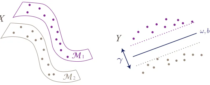
Figure 1: Illustration of a linearly separable embedding. Data in X are sampled from two different classes with supports M₁, M₂. The samples X are mapped to the coordinatesY with a low-dimensional embedding, where the two classes become linearly separable with marginγ with the hyperplane given byω,b.

Figure 1 shows an illustration of a linearly separable embedding of data samples from two classes. Manifold learning methods typically compute a low-dimensional embedding

Y of training data X in a pointwise manner, i.e., the coordinates yi are computed only

for the initially available training samples xi. However, in a classification problem, in

order to estimate the class label of a new data sample x of unknown class, x needs to be mapped to the low-dimensional domain of embedding as well. The construction of a function

f :H →_Rd _{that generalizes the learnt embedding to the whole space is known as the}

out-of-sample generalization problem. Smooth functions are commonly used for out-out-of-sample interpolation, e.g. as in (Qiao et al., 2013), (Peherstorfer et al., 2011).

Now letxbe a test sample drawn from the probability measureνm, hence, the true class

label ofx ism. In our study, we consider two basic classification schemes in the domain of embedding:

Linear classifier. The embeddings of the training samples are used to compute the

separating hyperplanes, i.e., the classifier parameters{ωmk} and {bmk}. Then, mapping x

to the low-dimensional domain as f(x)∈Rd, the class label of x is estimated as ˆC(x) = l

if there existsl∈ {1, . . . , M}such that

ωT_lkf(x) +blk>0, ∀k∈ {1, . . . , M} \ {l}. (4)

Note that the existence of such anl is not guaranteed in general for anyx, but for a given

x there cannot be more than one l satisfying the above condition. Then x is classified correctly if the estimated class label agrees with the true class label, i.e., ˆC(x) =l=m.

Nearest neighbor classification. The test sample x is assigned the class label of the

closest training point in the domain of embedding, i.e., ˆC(x) =Ci0, where

i0 = arg min

i=1,...,Nkyi−f(x)k.

(6)

vary regularly on each class support and we search for a lower bound on the probability of correctly classifying a new data sample in terms of the regularity of f, the separation of the embedding, and the sampling density. Then in Section 2.3, we study the classification performance for a particular type of interpolation functions, namely RBF interpolators, which is one of the most popular ones (Peherstorfer et al., 2011), (Chin and Suter, 2008). We focus particularly on Gaussian RBF interpolators in Section 2.4 and derive some results regarding the existence of an optimal kernel scale parameter. Lastly, we discuss our results in comparison with previous literature in Section 2.5.

In the results in Sections 2.2-2.4, we keep a generic formulation and simply treat the supports{Mm}as arbitrary bounded subsets ofH, each of which represents a different data

class. Nevertheless, from the perspective of manifold learning, our results are of interest especially when the data is assumed to have an underlying low-dimensional structure. In Section 2.5, we study the implications of our results for the setting where Mm are

low-dimensional manifolds. We then examine how the proposed bounds vary in relation to the intrinsic dimensions of {M_m}.

2.2 Out-of-Sample Interpolation with Regular Functions

Let f :H → Rd be an out-of-sample interpolation function such that f(xi) = yi for each

training sample xi, i = 1, . . . , N. Assume that f is Lipschitz continuous with constant

L > 0 when restricted to any one of the supports M_m; i.e., for any m ∈ {1, . . . , M} and any u, v∈ Mm

kf(u)−f(v)k ≤Lku−vk,

wherek · kdenotes above the`2-norm if the argument is inRd, and the norm induced from

the inner product in H if the argument is in H.

We will find a relation between the classification accuracy and the number of training samples via the covering number of the supportsMm. LetB(x)⊂H denote an open ball

of radius aroundx

B(x) ={u∈H :kx−uk< }.

The covering number N(, A) of a set A ⊂ H is defined as the smallest number of open ballsB of radius whose union contains A (Kulkarni and Posner, 1995)

N(, A) = inf{k:∃u1, . . . , uk∈Hs.t.A⊂ k

[

i=1

B(ui)}.

We assume that the supports Mm are totally bounded, i.e., Mm has a finite covering

number N(,Mm) for any >0.

We state below a lower bound for the probability of correctly classifying a sample x

drawn fromνm, in terms of the number of training samples drawn fromνm, the separation

of the embedding and the regularity of f.

Theorem 2 For some with 0 < ≤ γ/(2L), let the training set X contain at least Nm

samples drawn i.i.d. according to a probability measure νm such that

(7)

LetY be an embedding of the training samplesX that is linearly separable with margin larger

than γ, and let f be an interpolation function that is Lipschitz continuous with constant L

on the supportM_m. Then the probability of correctly classifying a test samplexdrawn from

νm independently from the training samples with the linear classifier (4) is lower bounded

as

P

ˆ

C(x) =m

≥1− N(/2,Mm)

2Nm

.

The proof of the theorem is given in Appendix A.1. Theorem 2 establishes a link between the classification performance and the separation of the embedding of the training samples. In particular, due to the condition ≤γ/(2L), the increase in the separation γ

allows a larger value for , provided that the interpolator regularity is not affected much. This reduces the covering number N(/2,M_m) in return and increases the probability of correct classification. Similarly, from the condition ≤γ/(2L), one can also observe that at a given separationγ, a smaller Lipschitz constantLfor the interpolation function allows the parameter to take a larger value. This reduces the covering number N(/2,M_m) and therefore increases the correct classification probability. Thus, choosing a more regular interpolator at a given separation helps improve the classification performance. If the

parameter is fixed, the Lipschitz constant of the interpolator is allowed to increase only proportionally to the separation margin. The condition that the interpolator must be sufficiently regular in comparison with the separation suggests that increasing the separation too much at the cost of impairing the interpolator regularity may degrade the classifier performance. In the case that the supportsM_mare low-dimensional manifolds, the covering number N(/2,Mm) increases at a geometric rate with the intrinsic dimension D of the

manifold, since a D-dimensional manifold is locally homeomorphic toRD. Therefore, from

the condition on the number of samples, Nm should increase at a geometric rate withD.

In Theorem 2 the probability of misclassification decreases with the number Nm of

training samples at a rate of O(N_m−1). In the rest of this section, we show that it is in fact possible to obtain an exponential convergence rate with linear and NN-classifiers under certain assumptions. We first present the following lemma.

Lemma 3 Let X = {xi}Ni=1 ⊂H be a set of training samples such that each xi is drawn

i.i.d. from one of the probability measures{νm}Mm=1. Letx be a test sample randomly drawn

according to the probability measure νm of class m. Let

A={xi∈ X :xi∈Bδ(x), xi∼νm} (5)

be the set of samples inX that are in aδ-neighborhood ofxand also drawn from the measure

νm. Assume that A contains |A|=Q samples. Then

P 

kf(x)−

1

Q X

xj∈A

f(xj)k ≤Lδ+ √

d 

≥1−2dexp

− Q

2 2L2_δ2

. (6)

Lemma 3 is proved in Appendix A.2. The inequality in (6) shows that as the numberQ

of training samples falling in a neighborhood of a test point x increases, the probability of the deviation of f(x) from its average within the neighborhood decreases. The parameter

(8)

When studying the classification accuracy in the main result below, we will use the following generalized definition of the linear separation.

Definition 4 Let Y be a linearly separable embedding with margin γ such that each pair

(k, l) of classes are separated with the hyperplanes given byωkl, bkl as defined in Definition

1. We say that the linear classifier given by{ωkl},{bkl}has aQ-mean separability margin of

γQ >0 if any choice of Q samples {yk,i}Qi=1⊂Y from class k andQ samples {yl,i}Qi=1 ⊂Y

from class l, l6=k, satisfies

ω_klT 1 Q

Q

X

i=1

yk,i

!

+bkl≥γQ/2

ω_klT 1 Q

Q

X

i=1

yl,i

!

+bkl≤ −γQ/2.

(7)

The above definition of separability is more flexible than the one in Definition 1. Clearly, an embedding that is linearly separable with margin γ has a Q-mean separability margin of γQ ≥ γ for any Q. As in the previous section, we consider that the test sample x is

classified with the linear classifier (4) in the low-dimensional domain, defined with respect to the set of hyperplanes given by{ωmk}and {bmk} as in (2) and (3).

In the following result, we show that an exponential convergence rate can be obtained with linear classifiers in supervised manifold learning. We define beforehand a parameter depending on δ, which gives the smallest possible measure of the δ-neighborhood Bδ(x) of

a pointx in support Mm.

ηm,δ := inf

x∈Mm

νm(Bδ(x)).

Theorem 5 Let X ={xi}Ni=1 ⊂H be a set of training samples such that each xi is drawn

i.i.d. from one of the probability measures {νm}Mm=1. Let Y be an embedding of X in Rd

that is linearly separable with a Q-mean separability margin larger than γQ. For a given

>0 and δ >0, let f be a Lipschitz-continuous interpolator such that

Lδ+

√

d≤ γQ

2 . (8)

Consider a test sample x randomly drawn according to the probability measure νm of class

m. If X contains at least Nm training samples drawn i.i.d. fromνm such that

Nm>

Q ηm,δ

,

then the probability of correctly classifying x with the linear classifier given in (4) is lower

bounded as

P

ˆ

C(x) =m

≥1−exp

−2 (Nmηm,δ−Q)

2

Nm

−2dexp

− Q

2 2L2_δ2

(9)

Theorem 5 is proved in Appendix A.3. The theorem shows how the classification ac-curacy is influenced by the separation of the classes in the embedding, the smoothness of the out-of-sample interpolant, and the number of training samples drawn from the density of each class. The condition in (8) points to the tradeoff between the separation and the regularity of the interpolation function. As the Lipschitz constant L of the interpolation function f increases, f becomes less “regular”, and a higher separation γQ is needed to

meet the condition. This is coherent with the expectation that, whenf becomes irregular, the classifier becomes more sensitive to the perturbations of the data, e.g., due to noise. The requirement of a higher separation is then for ensuring a larger margin in the linear classifier, which compensates for the irregularity off. From (8), it is also observed that the separation should increase with the dimension d as well, and also with , whose increase improves the confidence of the bound (9). Note that the condition in (8) implies also the following: When computing an embedding, it is not advisable to increase the separation of training data unconditionally. In particular, increasing the separation too much may violate the preservation of the geometry and yield an irregular interpolator. Hence, when designing a supervised dimensionality reduction algorithm, one must pay attention to the regularity of the resulting interpolator as much as the enhancement of the separation margin.

Next, we discuss the roles of the parametersQand δ. The term exp(−Q 2/(2L2δ2)) in the correct classification probability bound (9) shows that, for fixed δ, the confidence in-creases with the value ofQ. Meanwhile, due to the numerator of the term exp(−2 (Nmηm,δ−

Q)2/Nm), for a high confidence, the number of samples Nm should also be relatively big

with respect to Q to have a high overall confidence. Similarly, at fixed Q, δ should be made smaller to increase the confidence due to the term exp(−(Q 2₎_/₍₂_L2_δ2_{)), which then} reduces the parameter ηm,δ and eventually requires the number of samples Nm to take a

sufficiently large value in order to make the term exp(−2 (Nmηm,δ −Q)2/Nm) small and

have a high confidence. Therefore, these two parametersQ and δ behave in a similar way, and determine the relation between the number of samples and the correct classification probability, i.e., they indicate how largeNm should be in order to have a certain confidence

of correct classification.

Theorem 5 studies the setting where the class labels are estimated with a linear classi-fier in the domain of embedding. We also provide another result below that analyses the performance when a nearest-neighbor classifier is used in the domain of embedding.

such that

kyi−yjk< Dδ, if kxi−xjk ≤δ and Ci =Cj kyi−yjk> γ, if Ci6=Cj,

hence, nearby samples from the same class are mapped to nearby points, and samples from

different classes are separated by a distance of at least γ in the embedding.

For given >0 and δ >0, let f be a Lipschitz-continuous interpolation function such

that

Lδ+

√

d+D2δ≤

γ

(10)

Consider a test sample x randomly drawn according to the probability measure νm of

class m. IfX contains at least Nm training samples drawn i.i.d. fromνm such that

Nm>

Q ηm,δ

,

then the probability of correctly classifying x with nearest-neighbor classification in Rd is

lower bounded as

P

ˆ

C(x) =m

≥1−exp

−2 (Nmηm,δ−Q)

2

Nm

−2dexp

− Q

2 2L2_δ2

. (11)

Theorem 6 is proved in Appendix A.4. Theorem 6 is quite similar to Theorem 5 and can be interpreted similarly. Unlike in the previous result, the separability condition of the embedding is based on the pairwise distances of samples from different classes here. The condition (10) suggests that the result is useful when the parameterD2δis sufficiently small,

which requires the embedding to map nearby samples from the same class in the ambient space to nearby points.

In this section, we have characterized the regularity of the interpolation functions via their rates of variation when restricted to the supports Mm. While the results of this

section are generic in the sense that they are valid for any interpolation function with the described regularity properties, we have not examined the construction of such functions. In a practical classification problem where one uses a particular type of interpolation func-tions, one would also be interested in the adaptation of these results to obtain performance guarantees for the particular type of function used. Hence, in the following section we focus on a popular family of smooth functions; radial basis function (RBF) interpolators, and study the classification performance of this particular type of interpolators.

2.3 Out-of-Sample Interpolation with RBF Interpolators Here we consider an RBF interpolation functionf :H→_Rd _{of the form}

f(x) = [f1(x)f2(x) . . . fd(x)],

such that each component fk off is given by

fk(x) =

N

X

i=1

ck_i φ(kx−xik),

where φ :R→ R+ is a kernel function, cki ∈R are coefficients, and xi are kernel centers.

In interpolation with RBF functions, it is common to choose the set of kernel centers as the set of available data samples. Hence, we assume that the set of kernel centers {xi}Ni=1 is selected to be the same as the set of training samples X. We consider a setting where the coefficientsck_i are set such that f(xi) =yi, i.e.,f maps each training point inX to its

embedding previously computed with supervised manifold learning.

We consider the RBF kernel φ to be a Lipschitz continuous function with constant

Lφ>0, hence, for anyu, v∈R

(11)

Also, letC be an upper bound on the coefficient magnitudes such that for allk= 1, . . . , d

N

X

i=1

|ck_i| ≤ C.

In the following, we analyze the classification accuracy and extend the results in Section 2.2 to the case of RBF interpolators. We first give the following result, which probabilisti-cally bounds how much the value of the interpolatorf at a pointx randomly drawn from

νm may deviate from the average interpolator value of the training points of the same class

within a neighborhood of x.

Lemma 7 Let X = {xi}Ni=1 ⊂H be a set of training samples such that each xi is drawn

i.i.d. from one of the probability measures{νm}Mm=1. Letx be a test sample randomly drawn

according to the probability measure νm of class m. Let

A={xi∈ X :xi∈Bδ(x), xi∼νm} (12)

be the set of samples inX that are in aδ-neighborhood ofxand also drawn from the measure

νm. Assume that A contains |A|=Q samples. Then

P 

kf(x)−

1

Q X

xj∈A

f(xj)k ≤ √

dC(Lφδ+)



≥1−2Nexp −

(Q−1)2

2L2_φδ2

!

. (13)

The proof of Lemma 7 is given in Appendix A.5. The lemma states a result similar to the one in Lemma 3; however, is specialized to the case wheref is an RBF interpolator.

We are now ready to present the following main result.

Theorem 8 Let X ={xi}N_i₌₁ ⊂H be a set of training samples such that each xi is drawn

that is linearly separable with a Q-mean separability margin larger than γQ. For a given

>0 and δ >0, let f be an RBF interpolator such that √

dC(Lφδ+)≤

γQ

2 . (14)

Consider a test sample x randomly drawn according to the probability measure νm of class

m. If X contains at least Nm training samples drawn i.i.d. fromνm such that

Nm>

Q ηm,δ

,

then the probability of correctly classifying x with the linear classifier given in (4) is lower

bounded as

P

ˆ

C(x) =m

≥1−exp

−2 (Nmηm,δ−Q)

2

Nm

−2Nexp −(Q−1)

2 2L2

φδ2

!

(12)

The theorem is proved in Appendix A.6. The theorem bounds the classification accuracy in terms of the smoothness of the RBF interpolation function and the number of samples. The condition in (14) characterizes the compromise between the separation and the reg-ularity of the interpolator, which depends on the Lipschitz constant of the RBF kernels and the coefficient magnitude. As the Lipschitz constantLφand the coefficient magnitude

parameter C increase (i.e., f becomes less “regular”), a higher separation γQ is required

to provide a performance guarantee. When the separation margin of the embedding and the interpolator satisfy the condition in (14), the misclassification probability decays ex-ponentially as the number of training samples increases, similarly to the results in Section 2.2.

Theorem 8 studies the misclassification probability when the class labels in the low-dimensional domain are estimated with a linear classifier. We also present below a bound on the misclassification probability when the nearest-neighbor classifier is used in the low-dimensional domain.

such that

kyi−yjk< Dδ, if kxi−xjk ≤δ and Ci =Cj kyi−yjk> γ, if Ci6=Cj.

For given >0 and δ >0, let f be an RBF interpolator such that

√

dC(Lφδ+) +D2δ≤

γ

2. (16)

Consider a test sample x randomly drawn according to the probability measure νm of

class m. IfX contains at least Nm training samples drawn i.i.d. fromνm such that

Nm>

Q ηm,δ

,

then the probability of correctly classifying x with nearest-neighbor classification in Rd is

lower bounded as

P

ˆ

C(x) =m

≥1−exp

−2 (Nmηm,δ−Q)

2

Nm

−2Nexp −(Q−1)

2 2L2

φδ2

!

. (17)

Theorem 9 is proved in Appendix A.7. While it provides the exact convergence rate as in Theorem 8, the necessary condition in (16) includes also the parameterD2δ. Hence, if the

(13)

2.4 Optimizing the Scale of Gaussian RBF Kernels

In data interpolation with RBFs, it is known that the accuracy of interpolation is quite sensitive to the choice of the shape parameter for several kernels including the Gaussian kernel (Baxter, 1992). The relation between the shape parameter and the performance of interpolation has been an important problem of interest (Piret, 2007). In this section, we focus on the Gaussian RBF kernel, which is a popular choice for RBF interpolation due to its smoothness and good spatial localization properties. We study the choice of the scale parameter of the kernel within the context of classification.

We consider the RBF kernel given by

φ(r) =e−r

2

σ2,

whereσ is the scale parameter of the Gaussian function. We focus on the condition (14) in

Theorem 8 _√

dC(Lφδ+)≤γQ/2,

(or equivalently the condition (16) if the nearest neighbor classifier is used), which relates the interpolation function properties with the separation. In particular, for a given separation margin, this condition is satisfied more easily when the term on the left hand side of the inequality is smaller. Thus, in the following, we derive an expression for the left hand side of the above inequality by deriving the Lipschitz constantLφand the coefficient boundCin

terms of the scale parameter σ of the Gaussian kernel. We then study the scale parameter that minimizes √dC(Lφδ+).

Writing the condition f(xi) = yi in a matrix form for each dimension k = 1, . . . , d, we

have

Φck =yk, (18)

where Φ∈_RN×N _{is a matrix whose (}_{i, j}_{)-th entry is given by Φ}

ij =φ(kxi−xjk),ck∈RN×1

is the coefficient vector whosei-th entry isck

i, andyk∈RN×1 is the data coordinate vector

giving the k-th dimensions of the embeddings of all samples, i.e., yk_i =Yik. Assuming that

the embedding is computed with the usual scale constraint YTY =I, we have kykk = 1. The norm of the coefficient vector can then be bounded as

kckk ≤ kΦ−1kkykk=kΦ−1k. (19)

In the rest of this section, we assume that the data X are sampled from the Euclidean space, i.e.,H =Rn. We first use a result by Narcowich et al. (1994) in order to bound the

norm kΦ−1kof the inverse matrix. From (Narcowich et al., 1994, Theorem 4.1) we get1

kΦ−1k ≤β σ−neασ2, (20)

where α > 0 and β > 0 are constants depending on the dimension n and the minimum distance between the training pointsX (separation radius) (Narcowich et al., 1994). As the

1. The result stated in (Narcowich et al., 1994, Theorem 4.1) is adapted to our study by taking the measure as β(ρ) =δ(ρ−ρ0) so that the RBF kernel defined in (Narcowich et al., 1994, (1.1)) corresponds to a

(14)

`1-norm of the coefficient vector can be bounded askckk1 ≤

√

Nkckk, from (19) one can set the parameterC that upper bounds the coefficients magnitudes as

C=aσ−neασ2,

wherea=β√N.

Next, we derive a Lipschitz constant for the Gaussian kernelφ(r) in terms of σ. Setting the second derivative of φto zero

d2φ dr2 =e

−r2 σ2

4r2 σ4 −

2

σ2

= 0,

we get that the maximum value of |dφ/dr|is attained at r=σ/√2. Evaluating |dφ/dr|at this value, we obtain

Lφ= √

2e−12σ−1.

Now rewriting the condition (14) of the theorem, we have

√

dC(Lφδ+) =a1σ−n−1eασ

2

+a2σ−neασ

2

≤γQ/2,

wherea1 =

√

2d a e−1/2δanda2 =

√

d a . We thus determine the Gaussian scale parameter

σ that minimizes

F(σ) =a1σ−n−1eασ

2

+a2σ−neασ

2

.

First, notice that as σ→0 andσ → ∞, the functionF(σ)→ ∞. Therefore, it has at least one minimum. Setting

dF dσ =e

ασ2

σ−n−2 2αa2σ3+ 2αa1σ2−a2nσ−a1(n+ 1)

= 0,

we need to solve

2αa2σ3+ 2αa1σ2−a2nσ−a1(n+ 1) = 0. (21) The leading and the second-degree coefficients are positive, while the first-degree and the constant coefficients are negative in the above cubic polynomial. Then, the sum of the roots is negative and the product of the roots is positive. Therefore, there is one and only one positive root σopt, which is the unique minimizer ofF(σ).

The existence of an optimal scale parameter 0 < σopt < ∞ for the RBF kernel can be

intuitively explained as follows. When σ takes too small values, the support of the RBF function concentrated around the training points does not sufficiently cover the whole class supportsM_m. This manifests itself in (14) with the increase in the termLφ, which indicates

(15)

Remark: It is also interesting to observe how the optimal scale parameter changes with the number of samples N. In the study (Narcowich et al., 1994), the constants α

and β in (20) are shown to vary with the separation radius q at rates α = O(q−2) and

β =O(qn), where the separation radius q is proportional to the smallest distance between two distinct training samples. Then a reasonable assumption is that the separation radius

q should typically decrease at rate O(N−1/n) as N increases. Using this relation, we get that α and β should vary at rates α =O(N2/n) and β =O(N−1) with N. It follows that

a = β√N = O(N−1/2), and the parameters a1, a2 of the cubic polynomial in (21) also vary with N at rates a1 =O(N−1/2),a2 =O(N−1/2). The equation (21) inσ can then be rearranged as

b3σ3+b2σ2−b1σ−b0 = 0,

such that the constants vary with N at rates b3 = O(N2/n), b2 = O(N2/n), b1 = O(1),

b0 = O(1). We can then inspect how the roots of this equation change with N as N increases. Sinceb3 and b2 dominate the other coefficients for large N, three real roots will exist ifN is sufficiently large, two of which are negative and one is positive. The sum of the pairwise products of the roots is negative and it decays withN at rate O(N−2/n), and the product of the roots also decays with N. Then at least two of the roots must decay with

N. Meanwhile, the sum of the three roots isO(1) and negative. This shows that one of the negative roots is O(1), i.e., does not decay with N. From the product of three roots, we then observe that the product of the two decaying roots is O(N−2/n). However, their sum also decays at the same rate (from the sum of the pairwise products), which is possible if their dominant terms have the same rate and cancel each other. We conclude that both of the decaying roots vary at rateO(N−1/n), one of which is the positive root and the optimal valueσopt of the scale parameter.

This analysis shows that the scale parameter of the Gaussian kernel should be adapted to the number of training samples, and a smaller kernel scale must be preferred for a larger number of training samples. In fact, the relationσopt=O(N−1/n) is quite intuitive, as the

average or typical distance between two samples will also decrease at rateO(N−1/n) as the number of samples N increases in an n-dimensional space. Then the above result simply suggests that the kernel scale should be chosen as proportional to the average distance between the training samples.

2.5 Discussion of the Results in Relation with Previous Results

In Theorems 8 and 9, we have presented a result that characterizes the performance of classification with RBF interpolation functions. In particular, we have considered a setting where an RBF interpolator is fitted to each dimension of a low-dimensional embedding where different classes are separable. Our study has several links with RBF networks or least-squares regression algorithms. In this section, we interpret our findings in relation with previously established results.

(16)

ρ, the RBF network estimates a function ˆf of the form

ˆ

f(x) =

R

X

i=1

ciφ

kx−tik

σi

. (22)

The number of RBF terms R may be different from the number of samples N in general. The function ˆf minimizes the empirical error

ˆ

f = arg min

f N

X

j=1

(f(xj)−yj)2.

The function ˆf estimated from a finite collection of data samples is often compared to the regression function (Cucker and Smale, 2002)

fo(x) =

Z

Y

y dρ(y|x),

where dρ(y|x) is the conditional probability measure on Y. The regression function fo

minimizes the expected risk as

fo= arg min f

Z

X×Y

f(x)−y2 dρ.

As the probability measureρis not known in practice, the estimate ˆf offo is obtained from

data samples. Several previous works have characterized the performance of learning by studying the approximation error (Niyogi and Girosi, 1996), (Lin et al., 2014)

E[(fo−fˆ)2] =

Z

X

(fo(x)−fˆ(x))2dρX(x), (23)

where ρX is the marginal probability measure on X. This definition of the approximation

error can be adapted to our setting as follows. In our problem the distribution of each class is assumed to have a bounded support, which is a special case of modeling the data with an overall probability distributionρ. If the supportsMm are assumed to be nonintersecting,

the regression functionfo is given by

fo(x) = M

X

m=1

m Im(x),

which corresponds to the class labels m = 1, . . . , M, where Im is the indicator function of

the support Mm. It is then easy to show that the approximation error E[(fo−fˆ)2] can be

bounded as a constant times the probability of misclassification P( ˆC(x) 6=m). Hence, we can compare our misclassification probability bounds in Section 2.3 with the approximation error in other works.

(17)

|ci|is bounded. It is then shown that for data sampled from Rn, with probability greater

than 1−δ the approximation error in (23) can be bounded as

E[(fo−fˆ)2]≤O

1

R

+O r

Rnlog(RN)−log(δ)

N

!

, (24)

whereR is the number of RBF terms.

The analysis by Lin et al. (2014) considers families of RBF kernels that include the Gaussian function. Supposing that the regression function fo is of Sobolev class W2r, and that the number of RBF terms is given by R =Nn+2nr in terms of the number of samples

N, the approximation error is bounded as

E[(fo−fˆ)2]≤O(N−

2r

n+2r_log2₍_N₎₎_. ₍₂₅₎

Next, we overview the study by Hern´andez-Aguirre et al. (2002), which studies the performance of RBFs in a Probably Approximately Correct (PAC)-learning framework. For

X⊂_Rn_{, a family}_F _{of measurable functions from} _X_{to [0}_,_{1] is considered and the problem}

of approximating a target function f0 known only through examples with a function in ˆ

f ∈ F is studied. The authors use a previous result from (Vidyasagar, 1997) that relates the accuracy of empirical risk minimization to the covering number ofF and the number of samples. Combining this result with the bounds on covering number estimates of Lipschitz continuous functions (Kolmogorov and Tihomirov, 1961), the following result is obtained for PAC function learning with RBF neural networks with Gaussian kernel. Let the coefficients be bounded as |ci| ≤A, a common scale parameter be chosen as σi =σ, andE[|f0−fˆ|] be computed under a uniform probability measureρ. Then if the number of samples satisfies

N ≥ 8

ε2 log

√

2RnA e−1/2_σζ

, (26)

an approximation of the target function is obtained with accuracy parameter ε and confi-dence parameter ζ:

(18)

of the accuracy on the kernel scale parameter is monotonic in the bound (26); εdecreases asσ increases. Therefore, this bound does not guide the selection of the scale parameter of the RBF kernel, while the discussion in Section 2.4 (confirmed by the experimental results in Section 4.2) suggests the existence of an optimal scale.

Finally, we mention some results on the learning performance of regularized least squares regression algorithms. In (Caponnetto and De Vito, 2007) optimal rates are derived for the regularized least squares method in a Reproducing Kernel Hilbert Space (RKHS) in the minimax sense. It is shown that, under some hypotheses concerning the data probability measure and the complexity of the family of learnt functions, the maximum error (yielded by the worst distribution) obtained with the regularized least squares method converges at a rate ofO(1/N). Next, the work in (Steinwart et al., 2009) shows that, in regularized least squares regression over a RKHS, if the eigenvalues of the kernel integral operator decay sufficiently fast, and if the `∞-norms of regression functions can be bounded, the error of the classifier converges at a rate of up to O(1/N) with high probability. Steinwart et al. also examine the learning performance in relation with the exponent of the function norm in the regularization term and show that the learning rate is not affected by the choice of the exponent of the function norm.

We now overview the three bounds given in (24), (25), and (26) in terms of the depen-dence of the error on the number of samples. The results in (24) and (25) provide a useful bound only in the case where the number of samples N is larger than the number of RBF terms R, contrary to our study where we treat the case R=N. If it is assumed thatN is sufficiently larger thanR, the result in (24) predicts a rate of decay of onlyO(plog(N)/N) in the misclassification probability. The bound in (25) improves with the Sobolev regularity of the regression function; however, the dependence of the error on the number of samples is of a similar nature to the one in (24). Consideringεas a misclassification error parameter in the bound in (26), the error decreases at a rate of O(N−1/2) as the number of samples increases. The analysis in (Caponnetto and De Vito, 2007) and (Steinwart et al., 2009) also provide the similar rates of convergence of O(N−1). Meanwhile, our results in Theorems 8 and 9 predict an exponential decay in the misclassification probability as the number of samplesN increases (under the reasonable assumption thatNm=O(N) for each classm).

The reason why we arrive at a more optimistic bound is the specialization of the analysis to the considered particular setting, where the support of each class is assumed to be restricted to a totally bounded region in the ambient space, as well as the assumed relations between the separation margin of the embedding and the regularity of the interpolation function.

Another difference between these previous results and ours is the dependence on the dimension. The results in (24), (25), and (26) predict an increase in the error at the respective rates of O(√n), O(e−1/n), and O(√logn) with the ambient space dimension n. While these results assume that the data X ⊂ _Rn _{is in an Euclidean space of dimension}

(19)

In order to put the expressions (15), (17) in a more convenient form, let us reduce one parameter by setting Q=Nmηm,δ/2. Then the misclassification probability is of

O exp(−Nmηm,δ2 ) +Nexp −

Nmηm,δ2

L2

φδ2

!!

.

We can relate the dependence of this expression on the intrinsic dimension as follows. Since the supportsMm are assumed to be totally bounded, one can define a parameter Θ

that represents the “diameter” of Mm, i.e., the largest distance between any two points

on M_m. Then the measureηm,δ of the minimum ball of radius δ inMm is of O((δ/Θ)D),

whereDis the intrinsic dimension ofMm. Replacing this in the above expression gives the

probability of misclassification as

O exp

−Nmδ

2D

Θ2D

+Nexp −Nmδ D−22

L2_φΘD

!!

.

This shows that in order to retain the correct classification guarantee, as the intrinsic dimensionDgrows, the number of samplesNm should increase at a geometric rate withD.

In supervised manifold learning problems, data sets usually have a low intrinsic dimension, therefore, this geometric rate of increase can often be tolerated. Meanwhile the dimension of the ambient space is typically high, so that performance bounds independent of the ambient space dimension are of particular interest. Note that generalization bounds in terms of the intrinsic dimension have been proposed in some previous works as well (Bickel and Li, 2007), (Kpotufe, 2011), for the local linear regression and the K-NN regression problems.

3. Separability of Supervised Nonlinear Embeddings

In the results in Section 2, we have presented generalization bounds for classifiers based on linearly separable embeddings. One may wonder if the separability assumption is easy to satisfy when computing structure-preserving nonlinear embeddings of data. In this section, we try to answer this question by focusing on a particular family of supervised dimensionality reduction algorithms, i.e., supervised Laplacian eigenmaps embeddings, and analyze the conditions of separability. We first discuss the supervised Laplacian eigenmaps embeddings in Section 3.1 and then present results in Section 3.2 about the linearly separability of these embeddings.

3.1 Supervised Laplacian Eigenmaps Embeddings

Let X = {xi}iN=1 ⊂ H be a set of training samples, where each xi belongs to one of M

(20)

data samples xi, xj. We denote the edge weight as wij > 0. The weights wij are usually

determined as a positive and monotonically decreasing function of the distance between xi

and xj inH, where the Gaussian function is a common choice. Nevertheless, we maintain

a generic formulation here without making any assumption on the neighborhood or weight selection strategies.

Now let Gw and Gb represent two subgraphs of G, which contain the edges of G that

are respectively within the same class and between different classes. Hence, Gw contains

an edge i∼w j between samples xi and xj, if i∼ j and Ci =Cj. Similarly, Gb contains

an edge i ∼_b j if i ∼ j and Ci 6= Cj. We assume that all vertices of G are contained in

bothGw andGb; and thatGw has exactlyM connected components such that the training

samples in each class form a connected component2. We also assume that Gw and Gb do

not contain any isolated vertices; i.e., each data samplexi has at least one neighbor in both

graphs.

The N ×N weight matrices Ww and Wb ofGw and Gb have entries as follows.

Ww(i, j) =

wij ifi∼j and Ci =Cj

0 otherwise

Wb(i, j) =

wij ifi∼j and Ci 6=Cj

0 otherwise Letdw(i) and db(i) denote the degrees of xi inGw andGb

dw(i) =

X

j∼wi

wij, db(i) =

X

j∼bi

wij,

andDw,Dbdenote theN×N diagonal degree matrices given byDw(i, i) =dw(i),Db(i, i) =

db(i). The normalized graph Laplacian matricesLw and Lb ofGw andGb are then defined

as

Lw :=Dw−1/2(Dw−Ww)Dw−1/2, Lb :=D

−1/2

b (Db−Wb)D

−1/2

b .

Supervised extensions of the Laplacian eigenmaps and LPP algorithms seek ad-dimensional embedding of the data set X, such that each xi is represented by a vector yi ∈Rd×1.

De-noting the new data matrix asY = [y1y2 . . . yN]T ∈RN×d, the coordinates of data samples

are computed by solving the problem

“Minimize tr(YTLwY) while maximizing tr(YTLbY).” (28)

The reason behind this formulation can be explained as follows. For a graph Laplacian matrix L = D−1/2(D−W)D−1/2, where D and W are respectively the degree and the weight matrices, defining the coordinates Z =D−1/2_Y _{normalized with the vertex degrees,} we have

tr(YTL Y) = tr(ZT(D−W)Z) =X

i∼j

kzi−zjk2wij, (29)

(21)

whereziis thei-th row ofZ giving the normalized coordinates of the embedding of the data

sample xi. Hence, the problem in (28) seeks a representation Y that maps nearby samples

in the same class to nearby points, while mapping nearby samples from different classes to distant points. In fact, when the samplesxi are assumed to come from a manifold M, the

termyTLy is the discrete equivalent of

Z

M

k∇f(x)k2dx,

wheref :M →_Ris a continuous function on the manifold that extends the one-dimensional coordinatesyto the whole manifold. Hence, the term tr(YTLY) captures the rate of change of the learnt coordinate vectorsY over the underlying manifold. Then, in a setting where the samples of different classes come fromMdifferent manifolds{Mm}Mm=1, the formulation in (28) looks for a function that has a slow variation on each manifoldM_m, while having a fast variation “between” different manifolds.

The supervised learning problem in (28) has so far been studied by several authors with slight variations in their problem formulations. Raducanu and Dornaika (2012) minimize a weighted difference of the within-class and between-class similarity terms in (28) in order to learn a nonlinear embedding. Meanwhile, linear dimensionality reduction methods pose the manifold learning problem as the learning of a linear projection matrixP ∈_Rd×n_{; therefore,}

solve the problem in (28) under the constraintyi =P xi, wherexi∈Rn×1 and d < n. Hua

et al. (2012) formulate the problem as the minimization of the difference of the within-class and the between-within-class similarity terms in (28) as well. Thus, their algorithm can be seen as the linear version of the method by Raducanu and Dornaika (2012). Sugiyama (2007) proposes an adaptation of the Fisher discriminant analysis algorithm to preserve the local structures of data. Data sample pairs are weighted with respect to their affinities in the construction of the within-class and the between-class scatter matrices in Fisher discriminant analysis. Then the trace of the ratio of the between-class and the within-class scatter matrices is maximized to learn a linear embedding. Meanwhile, the within-class and the between-class local scatter matrices are closely related to the two terms in (28) as shown by Yang et al. (2011). The terms YTLwY and YTLbY, when evaluated under the

constraint yi = P xi, become equal to the locally weighted within-class and between-class

scatter matrices of the projected data. Cui and Fan (2012) and Wang and Chen (2009) propose to maximize the ratio of the between-class and the within-class local scatters in the learning. Yang et al. (2011) optimize the same objective function, while they construct the between-class graph only on the centers of mass of the classes. Zhang et al. (2012) similarly optimize a Fisher metric to maximize the ratio of the between- and within-class scatters; however, the total scatter is also taken into account in the objective function in order to preserve the overall manifold structure.

All of the above methods use similar formulations of the supervised manifold learning problem and give comparable results. In our study, we base our analysis on the following formal problem definition

min

Y tr(Y

T_L

wY)−µtr(YTLbY) subject to YTY =I, (30)

(22)

d×d identity matrix and µ > 0 is a parameter adjusting the weights of the two terms. The condition YTY = I is a commonly used constraint to remove the scale ambiguity of the coordinates. The solution of the problem (30) is given by the firstdeigenvectors of the matrix

Lw−µLb

corresponding to its smallest eigenvalues.

Our purpose in this section is then to theoretically study the linear separability of the learnt coordinates of training data, with respect to the definition of linear separability given in (1). In the following, we determine some conditions on the graph properties and the weight parameterµthat ensure the linear separability. We derive lower bounds on the margin γ and study its dependence on the model parameters. Let us give beforehand the following definitions about the graphsGw andGb.

Definition 10 The volume of the subgraph of Gw that corresponds to the connected

com-ponent containing samples from class k is

Vk :=

X

i:Ci=k

dw(i).

We define the maximal within-class volume as

Vmax := max k=1,...,MVk.

The volume of the component of Gb containing the edges between the samples of classes k

and l is3

V_klb := X

i∼bj Ci=k,Cj=l

2wij.

We then define the maximal pairwise between-class volume as

V_maxb := max

k6=l V b kl.

In a connected graph, the distance between two vertices xi and xj is the number of

edges in a shortest path joiningxi and xj. The diameter of the graph is then given by the

maximum distance between any two vertices in the graph (Chung, 1996). We define the diameter of the connected component of Gw corresponding to class kas follows.

Definition 11 For any two vertices xi and xj such that Ci =Cj =k, consider a

within-class shortest path joining xi and xj, which contains samples only from class k. Then the

diameter Dk of the connected component of Gw corresponding to class k is the maximum

number of edges in the within-class shortest path joining any two vertices xi and xj from

class k.

Definition 12 The minimum edge weight within class k is defined as

wmin,k := min

i∼wj Ci=Cj=k

wij.

3. In order to keep the analogy with the definition ofVk, a 2 factor is introduced in this expression as each

(23)

3.2 Separability Bounds for Two Classes

We now present a lower bound for the linear separability of the embedding obtained by solving (30) in a setting with two classes Ci ∈ {1,2}. We first show that an embedding

of dimension d = 1 is sufficient to achieve linear separability for the case of two classes. We then derive a lower bound on the separation in terms of the graph parameters and the algorithm parameter µ.

Consider a one-dimensional embedding Y =y = [y1y2 . . . yN]T ∈RN×1, where yi ∈R

is the coordinate of the data samplexi in the one-dimensional space. The coordinate vector

yis given by the eigenvector ofLw−µLb corresponding to its smallest eigenvalue. We begin

with presenting the following result, which states that the samples from the two classes are always mapped to different halves (nonnegative or nonpositive) of the real line.

Lemma 13 The learnt embeddingy of dimension d= 1 satisfies

yi ≤0 if Ci = 1 (or respectively Ci=2)

yi ≥0 if Ci = 2 (or respectively Ci=1)

for anyµ >0 and for any choice of the graph parameters.

Lemma 13 is proved in Appendix B.1. The lemma states that in one-dimensional embed-dings of two classes, samples from different classes always have coordinates with different signs. Therefore, the hyperplane given by ω = 1, b= 0 separates the data asωTyi ≤0 for

Ci = 1 and ωTyi ≥0 for Ci = 2 (since the embedding is one dimensional, the vector ω is

a scalar in this case). However, this does not guarantee that the data is separable with a positive margin γ >0. In the following result, we show that a positive margin exists and give a lower bound on it. In the rest of this section, we assume without loss of generality that classes 1 and 2 are respectively mapped to the negative and positive halves of the real axis.

Theorem 14 Defining the normalized data coordinatesz=Dw−1/2y, let

z1,max:= max

i:Ci=1zi z2,min:= mini:Ci=2zi

denote the maximum and minimum coordinates that classes1 and2 are respectively mapped

to with a one-dimensional embedding learnt with supervised Laplacian eigenmaps. We also define the parameters

wmin= min k∈{1,2}

wmin,k

Dk

, βi =

dw(i)

db(i)

, βmax = max

i βi,

where Dk is the diameter of the graph corresponding to class k as defined in Definition

11. Then, if the weight parameter is chosen such that 0 < µ < wmin/(βmaxVmaxb ), any

supervised Laplacian embedding of dimension d ≥ 1 is linearly separable with a positive

margin lower bounded as below:

z2,min−z1,max≥

1

√

Vmax



1− s

µβmaxVmaxb

wmin



(24)

The proof of Theorem 14 is given in Appendix B.2. The proof is based on a variational characterization of the eigenvector of Lw −µLb corresponding to its smallest eigenvalue,

whose elements are then bounded in terms of the parameters of the graph such as the diameters and volumes of its connected components.

Theorem 14 states that an embedding learnt with the supervised Laplacian eigenmaps method makes two classes linearly separable if the weight parameterµis chosen sufficiently small. In particular, the theorem shows that, for any 0 < δ < Vmax−1/2, a choice of the

weight parameterµsatisfying

0< µ≤ wmin

βmaxVmaxb

1−pVmaxδ

2

guarantees a separation ofz2,min−z1,max ≥δ between classes 1 and 2 atd= 1. Here, we

use the symbol δ to denote the separation in the normalized coordinates z. In practice, either one of the normalized eigenvectors z or the original eigenvectors y can be used for embedding the data. If the original eigenvectorsy are used, due to the relation y=D1w/2z,

we can lower bound the separation as y2,min−y1,max ≥

p

dw,min(z2,min−z1,max) where

dw,min= minidw(i). Thus, for any embedding of dimensiond≥1, there exists a hyperplane

that results in a linear separation with a marginγ of at least

γ ≥

s

dw,min

Vmax



1− s

µβmaxVmaxb

wmin



.

Next, we comment on the dependence of the separation on µ. The inequality in (31) shows that the lower bound on the separation z2,min−z1,max has a variation ofO(1−

√

µ) with the weight parameterµ. The fact that the separation decreases with the increase inµ

seems counterintuitive at first; this parameter weights the between-class dissimilarity in the objective function. This can be explained as follows. Whenµis high, the algorithm tries to increase the distance between neighboring samples from different classes as much as possible by moving them away from the origin (remember that different classes are mapped to the positive and the negative sides of the real line). However, since the normalized coordinate vectorz has to respect the equality zTDwz= 1, the total squared norm of the coordinates

cannot be arbitrarily large. Due to this constraint, setting µ to a high value causes the algorithm to map non-neighboring samples from different classes to nearby coordinates close to the origin. This occurs since the increase inµ reduces the impact of the first term

yTLwyin the overall objective and results in an embedding with a weaker link between the

samples of the same class. This causes a polarization of the data and eventually reduces the separation. Hence, theµparameter should be carefully chosen and should not take too large values.

(25)

Corollary 15 The distance between the supports of the first and the second classes and the origin in a one-dimensional embedding is lower bounded in terms of the separation between the two classes as

min{|z1,max|, |z2,min|} ≥

1 2

βmin

βmax

(z2,min−z1,max) where

βmin= min

i βi, βmax= maxi βi.

Corollary 15 is proved in Appendix B.3. The proof is based on a Lagrangian formulation of the embedding as a constrained optimization problem, which then allows us to establish a link between the separation and the individual distances of class supports to the origin. The corollary states a lower bound on the portion of the overall separation lying in the negative or the positive sides of the real line. In particular, if the vertex degrees are equal for all samples in Gw andGb (which is the case, for instance, if all vertices have the same number

of neighbors and a constant weight of wij = 1 is assigned to the edges), sinceβmin =βmax,

the portions of the overall separation in the positive and negative sides of the real line will be equal.

We have examined the linear separability of supervised Laplacian embeddings for the case of two classes in this section. An extension of these results to the case of multiple classes under some assumptions is available in the accompanying technical report (Vural and Guillemot, 2016b).

4. Experimental Results

In this section, we present results on synthetical and real data sets. We compare several supervised manifold learning methods and study their performances in relation with our theoretical results.

4.1 Separability of Embeddings with Supervised Manifold Learning

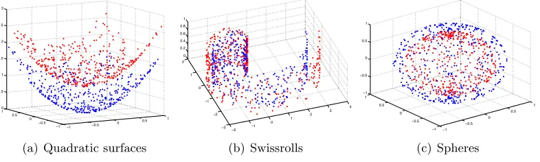
We first present results on synthetical data in order to study the embeddings obtained with supervised dimensionality reduction. We test the supervised Laplacian eigenmaps algorithm in a setting with two classes. We generate samples from two nonintersecting and linearly nonseparable surfaces in R3 that represent two different classes. We experiment on three

different types of surfaces; namely, quadratic surfaces, Swiss rolls and spheres. The data sampled from these surfaces are shown in Figure 2. We chooseN = 200 samples from each class. We construct the graph Gw by connecting each sample to its K-nearest neighbors

from the same class, where K is chosen between 20 and 30. The graph Gb is constructed

(26)

−1 −0.5 0 0.5 1 −1 −0.5 0 0.5 1 0 0.5 1 1.5 2 2.5 3

(a) Quadratic surfaces

−2 −1 0 1 2 3 4 −3 −2 −1 0 1 2 0 0.2 0.4 0.6 0.8 1 (b) Swissrolls −1 −0.5 0 0.5 1 −1 −0.5 0 0.5 1 −1 −0.5 0 0.5 1 (c) Spheres

Figure 2: Data sampled from two-dimensional synthetical surfaces. Red and blue colors represent two different classes.

−0.02 −0.015 −0.01 −0.005 0 0.005 0.01 0.015 0.02 −1 −0.8 −0.6 −0.4 −0.2 0 0.2 0.4 0.6 0.8 1

(a) 1-D embedding

−0.02 −0.015 −0.01 −0.005 0 0.005 0.01 0.015 0.02 −0.025 −0.02 −0.015 −0.01 −0.005 0 0.005 0.01 0.015 0.02 0.025

(b) 2-D embedding

−0.02−0.015−0.01−0.005 0 0.005 0.01 0.015 0.02 −0.04 −0.02 0 0.02 0.04 −0.03 −0.02 −0.01 0 0.01 0.02 0.03

(c) 3-D embedding

Figure 3: Supervised Laplacian embeddings of data sampled from quadratic surfaces.

(to have a visually clear embedding for the purpose of illustration). Similar results are obtained on the Swiss roll and the spherical surface. One can observe that the data samples that were initially linearly nonseparable become linearly separable when embedded with the supervised Laplacian eigenmaps algorithm. The two classes are mapped to different (positive or negative) sides of the real line in Figure 3(a) as predicted by Lemma 13. The separation in the 2-D and 3-D embeddings in Figure 3 is close to the separation obtained with the 1-D embedding.

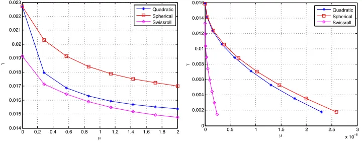
We then compute and plot the separation obtained at different values of µ. Figure 4(a) shows the experimental value of the separation γ =z2,min−z1,max obtained with the 1-D

embedding for the three types of surfaces. Figure 4(b) shows the theoretical upper bound forµin Theorem 14 that guarantees a separation of at leastγ. Both the experimental value and the theoretical bound for the separationγ decrease with the increase in the parameter

(27)

0 0.2 0.4 0.6 0.8 1 1.2 1.4 1.6 1.8 2 0.014

0.015 0.016 0.017 0.018 0.019 0.02 0.021 0.022 0.023

µ

γ

Quadratic Spherical Swissroll

(a) Experimental value of the separationγ

0 0.5 1 1.5 2 2.5 3

x 10−6 0

0.002 0.004 0.006 0.008 0.01 0.012 0.014 0.016

µ

γ

Quadratic Spherical Swissroll

(b) Theoretical upper bound forµthat guar-antees a separation of at leastγ

Figure 4: Variation of the separation γ between the two classes with the parameter µ for the synthetic data sets

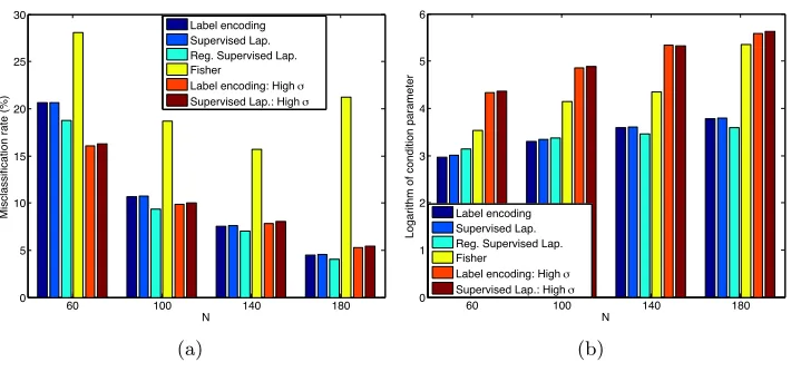
fast rate of decrease for the separation due to (31). Comparing Figures 4(a) and 4(b), one observes that the theoretical bounds for the separation are numerically more pessimistic than their experimental values, which is a result of the fact that our results are obtained with a worst-case analysis. Nevertheless, the theoretical bounds capture well the actual variation of the separation margin with µ.

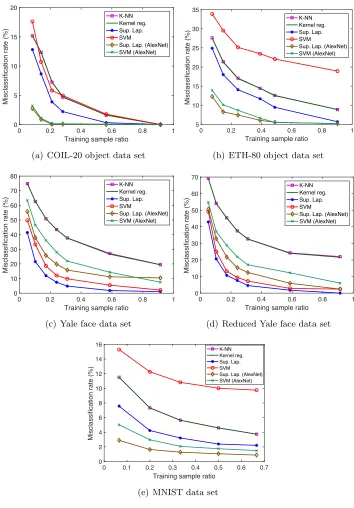
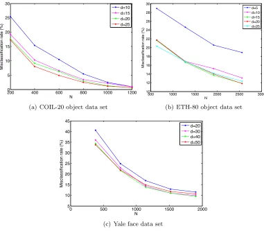
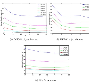
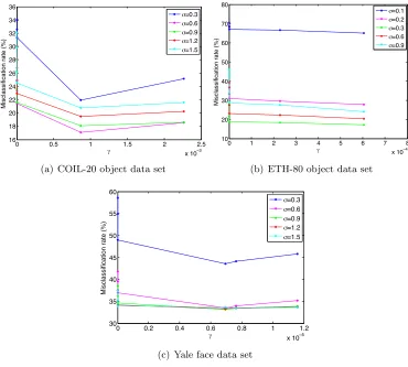
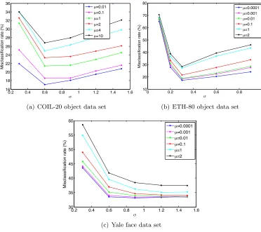
4.2 Classification Performance of Supervised Manifold Learning Algorithms We now study the overall performance of classification obtained in a setting with super-vised manifold learning, where the out-of-sample generalization is achieved with smooth RBF interpolators. We evaluate the theoretical results of Section 2 on several real data sets: the COIL-20 object database (Nene et al., 1996), the Yale face database (Georghi-ades et al., 2001), the ETH-80 object database (Leibe and Schiele, 2003), and the MNIST handwritten digit database (LeCun et al., 1998). The COIL-20, Yale face, ETH-80, and MNIST databases contain a total of 1420, 2204, 3280, and 70046 images from 20, 38, 8, and 10 image classes respectively. The images in the COIL-20, Yale and ETH-80 data sets are converted to greyscale, normalized, and downsampled to a resolution of respectively 32×32, 20×17, and 20×20 pixels.

4.2.1 Comparison of Supervised Manifold Learning to Baseline Classifiers

(28)

0 0.2 0.4 0.6 0.8 1 Training sample ratio

0 5 10 15 20

Misclassification rate (%)

K-NN Kernel reg. Sup. Lap. SVM

Sup. Lap. (AlexNet) SVM (AlexNet)

(a) COIL-20 object data set

0 0.2 0.4 0.6 0.8 1

Training sample ratio 5

10 15 20 25 30 35

(b) ETH-80 object data set