SGDLibrary: A MATLAB library for stochastic optimization
algorithms
Hiroyuki Kasai [email protected]
Graduate School of Informatics and Engineering The University of Electro-Communications Tokyo, 182-8585, Japan
Editor:Geoff Holmes
Abstract
We consider the problem of finding the minimizer of a functionf :Rd→Rof the finite-sum
form minf(w) = 1/nPn
i fi(w). This problem has been studied intensively in recent years
in the field of machine learning (ML). One promising approach for large-scale data is to use a stochastic optimization algorithm to solve the problem. SGDLibrary is a readable, flexible and extensible pure-MATLAB library of a collection of stochastic optimization algorithms. The purpose of the library is to provide researchers and implementers a comprehensive evaluation environment for the use of these algorithms on various ML problems.
Keywords: Stochastic optimization, stochastic gradient, finite-sum minimization prob-lem, large-scale optimization problem
1. Introduction
This work aims to facilitate research on stochastic optimization for large-scale data. We particularly address a regularized finite-sum minimization problem defined as
min
w∈Rd
f(w) := 1
n
n
X
i=1
fi(w) =
1
n
n
X
i=1
L(w, xi, yi) +λR(w), (1)
wherew∈Rdrepresents the model parameter andndenotes the number of samples (x i, yi).
L(w, xi, yi) is the loss function andR(w) is the regularizer with the regularization parameter
λ≥ 0. Widely diverse machine learning (ML) models fall into this problem. Considering
L(w, xi, yi) = (wTxi −yi)2, xi ∈ Rd, yi ∈ R and R(w) = kwk22, this results in an `2
-norm regularized linear regression problem (a.k.a. ridge regression) for ntraining samples (x1, y1),· · ·,(xn, yn). In the case of binary classification with the desired class label yi ∈ {+1,−1} and R(w) = kwk1, an `1-norm regularized logistic regression (LR) problem is
obtained as fi(w) = log(1 + exp(−yiwTxi)) +λkwk1, which encourages the sparsity of the
solution of w. Other problems covered are matrix completion, support vector machines (SVM), and sparse principal components analysis, to name but a few.
Full gradient descent (a.k.a. steepest descent) with a step-size η is the most straight-forward approach for (1), which updates as wk+1 ← wk−η∇f(wk) at the k-th iteration.
However, this is expensive whenn is extremely large. In fact, one needs a sum ofn calcu-lations of the inner productwTxi in the regression problems above, leading toO(nd) cost
overall per iteration. For this issue, a popular and effective alternative isstochastic gradient
c
2018 Hiroyuki Kasai.
descent (SGD), which updates aswk+1 ←wk−η∇fi(wk) for the i-th sample uniformly at
random (Robbins and Monro, 1951; Bottou, 1998). SGD assumes an unbiased estimator
of the full gradient as Ei[∇fi(wk)] = ∇f(wk). As the update rule represents, the
calcu-lation cost is independent of n, resulting in O(d) per iteration. Furthermore, mini-batch
SGD (Bottou, 1998) calculates 1/|Sk|Pi∈Sk∇fi(wk), whereSk is the set of samples of size
|Sk|. SGD needs adiminishing step-size algorithm to guarantee convergence, which causes a severe slow convergence rate (Bottou, 1998). To accelerate this rate, we have two active research directions in ML;Variance reduction (VR) techniques (Johnson and Zhang, 2013; Roux et al., 2012; Shalev-Shwartz and Zhang, 2013; Defazio et al., 2014; Nguyen et al., 2017) that explicitly or implicitly exploit a full gradient estimation to reduce the variance of the noisy stochastic gradient, leading to superior convergence properties. Another promising direction is to modify deterministic second-order algorithms into stochastic settings, and solve the potential problem of first-order algorithms for ill-conditioned problems. A direct extension of quasi-Newton (QN) is known as online BFGS (Schraudolph et al., 2007). Its variants include a regularized version (RES) (Mokhtari and Ribeiro, 2014), a limited mem-ory version (oLBFGS) (Schraudolph et al., 2007; Mokhtari and Ribeiro, 2015), a stochastic QN (SQN) (Byrd et al., 2016), an incremental QN (Mokhtari et al., 2017), and a non-convex version. Lastly, hybrid algorithms of the SQN with VR are proposed (Moritz et al., 2016; Kolte et al., 2015). Others include (Duchi et al., 2011; Bordes et al., 2009).
The performance of stochastic optimization algorithms is strongly influenced not only by the distribution of data but also by the step-size algorithm (Bottou, 1998). Therefore, we often encounter results that are completely different from those in papers in every exper-iment. Consequently, an evaluation framework to test and compare the algorithms at hand is crucially important for fair and comprehensive experiments. One existing tool is Light-ning(Blondel and Pedregosa, 2016), which is a Python library for large-scale ML problems. However, its supported algorithms are limited, and the solvers and the problems such as classifiers are mutually connected. Moreover, the implementations utilize Cython, which is a C-extension for Python, for efficiency. Subsequently, they decrease users’ readability of code, and also make users’ evaluations and extensions more complicated. SGDLibrary is a readable, flexible and extensible pure-MATLAB library of a collection of stochastic optimization algorithms. The library is also operable on GNU Octave. The purpose of the library is to provide researchers and implementers a collection of state-of-the-art stochas-tic optimization algorithms that solve a variety of large-scale optimization problems such as linear/non-linear regression problems and classification problems. This also allows re-searchers and implementers to easily extend or add solvers and problems for further evalu-ation. To the best of my knowledge, no report in the literature and no library describe a comprehensive experimental environment specialized for stochastic optimization algorithms. The code is available athttps://github.com/hiroyuki-kasai/SGDLibrary.
2. Software architecture
Problem descriptor: The problem descriptor, denoted asproblem, specifies the problem of interest with respect to w, noted as win the library. This is implemented by MATLAB
classdef. The user does nothing other than calling a problem definition function, for instance,logistic_regression() for the`2-norm regularized LR problem. Each problem
definition includes the functions necessary for solvers; (i) (full) cost function f(w), (ii) mini-batch stochastic derivative v=1/|S|∇fi∈S(w) for the set of samplesS. (iii) stochastic
Hessian (Bordes et al., 2009), and (iv) stochastic Hessian-vector product for a vector v. The built-in problems include, for example, `2-norm regularized multidimensional linear
regression, `2-norm regularized linear SVM, `2-norm regularized LR, `2-norm regularized
softmax classification (multinomial LR), `1-norm multidimensional linear regression, and `1-norm LR. The problem descriptor provides additional specific functions. For example,
the LR problem includes the prediction and the classification accuracy calculation functions.
Optimization solver: The optimization solver implements the main routine of the stochas-tic optimization algorithm. Once a solver function is called with one selected problem de-scriptorproblem as the first argument, it solves the optimization problem by calling some corresponding functions viaproblem such as the cost function and the stochastic gradient calculation function. Examples of the supported optimization solvers in the library are listed in categorized groups as; (i)SGD methods: Vanila SGD (Robbins and Monro, 1951), SGD with classical momentum, SGD with classical momentum with Nesterov’s accelerated gra-dient (Sutskever et al., 2013), AdaGrad (Duchi et al., 2011), RMSProp, AdaDelta, Adam, and AdaMax, (ii) Variance reduction (VR) methods: SVRG (Johnson and Zhang, 2013), SAG (Roux et al., 2012), SAGA (Defazio et al., 2014), and SARAH (Nguyen et al., 2017), (iii)Second-order methods: SQN (Bordes et al., 2009), oBFGS-Inf (Schraudolph et al., 2007; Mokhtari and Ribeiro, 2015), oBFGS-Lim (oLBFGS) (Schraudolph et al., 2007; Mokhtari and Ribeiro, 2015), Reg-oBFGS-Inf (RES) (Mokhtari and Ribeiro, 2014), and Damp-oBFGS-Inf, (iv) Second-order methods with VR: SVRG-LBFGS (Kolte et al., 2015), SS-SVRG (Kolte et al., 2015), and SVRG-SQN (Moritz et al., 2016), and (v) Else: BB-SGD and SVRG-BB. The solver function also receives optional parameters as the second argument, which forms astruct, designated asoptions in the library. It contains elements such as the maximum number of epochs, the batch size, and the step-size algorithm with an initial step-size. Finally, the solver function returns to the caller the final solutionwand rich statistical information, such as a record of the cost function values, the optimality gap, the processing time, and the number of gradient calculations.
Others: SGDLibrary accommodates auser-defined step-size algorithm. This
accommoda-tion is achieved by setting asoptions.stepsizefun=@my_stepsize_alg, which is delivered to solvers. Additionally, when the regularizer R(w) in the minimization problem (1) is a non-smooth regularizer such as the `1-norm regularizer kwk1, the solver calls the prox-imal operator as problem.prox(w,stepsize), which is the wrapper function defined in each problem. The `1-norm regularized LR problem, for example, calls the soft-threshold
function asw = prox(w,stepsize)=soft_thresh(w,stepsize*lambda), wherestepsize
is the step-sizeη and lambdais the regularization parameter λ >0 in (1).
3. Tour of the SGDLibrary
We embark on a tour of SGDLibrary exemplifying the `2-norm regularized LR problem.
The LR model generates n pairs of (xi, yi) for an unknown model parameter w, where xi
is an inputd-dimensional vector and yi ∈ {−1,1}is the binary class label, asP(yi|xi, w) =
1/(1 + exp(−yiwTxi)). The problem seeks w that fits the regularized LR model to the
generated data (xi, yi). This problem is cast as a minimization problem as minf(w) :=
1/nPn
i=1log[1 + exp(−yiwTxi)] +λ/2kwk2.The code for this problem is in Listing 1.
1 % g e n e r a t e s y n t h e t i c 300 s a m p l e s of d i m e n s i o n 3 for l o g i s t i c r e g r e s s i o n
2 d = l o g i s t i c _ r e g r e s s i o n _ d a t a _ g e n e r a t o r (300 ,3) ; 3 % d e f i n e l o g i s t i c r e g r e s s i o n p r o b l e m
4 p r o b l e m = l o g i s t i c _ r e g r e s s i o n ( d . x_train , d . y_train , d . x_test , d . y _ t e s t ) ; 5
6 o p t i o n s . w _ i n i t = d . w _ i n i t ; % set i n i t i a l v a l u e
7 o p t i o n s . s t e p _ i n i t = 0 . 0 1 ; % set i n i t i a l s t e p s i z e
8 o p t i o n s . v e r b o s e = 1; % set v e r b o s e m o d e
9 [ w_sgd , i n f o _ s g d ] = sgd ( problem , o p t i o n s ) ; % p e r f o r m SGD s o l v e r
10 [ w_svrg , i n f o _ s v r g ] = s v r g ( problem , o p t i o n s ) ; % p e r f o r m S V R G s o l v e r
11 [ w_svrg , i n f o _ s v r g ] = sqn ( problem , o p t i o n s ) ; % p e r f o r m SQN s o l v e r
12 % d i s p l a y c o s t vs . n u m b e r of g r a d i e n t e v a l u a t i o n s
13 d i s p l a y _ g r a p h (’ g r a d _ c a l c _ c o u n t ’,’ c o s t ’,{’ SGD ’,’ S V R G ’} ,... 14 { w_sgd , w _ s v r g } ,{ i n f o _ s g d , i n f o _ s v r g }) ;
Listing 1: Demonstration code for logistic regression problem.
First, we generate train/test datasetsdusinglogistic_regression_data_generator(), where the input feature vector is withn= 300 andd= 3. yi ∈ {−1,1}is its class label. The
LR problem is defined by calling logistic_regression(), which internally contains the functions for cost value, the gradient and the Hessian. This is stored inproblem. Then, we execute solvers, i.e., SGD and SVRG, by calling solver functions, i.e.,sgd()andsvrg()with
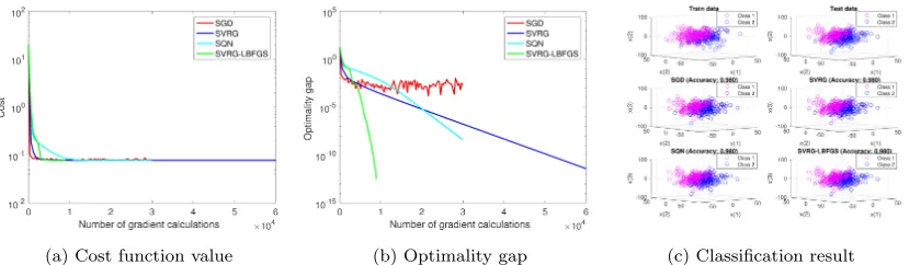
problemand options after setting some options into theoptionsstruct. They return the final solutions of{w_sgd,w_svrg} and the statistical information{info_sgd,info_svrg}. Finally,display_graph()visualizes the behavior of the cost function values in terms of the number of gradient evaluations. It is noteworthy that each algorithm requires a different number of evaluations of samples in each epoch. Therefore, it is common to use this value to evaluate the algorithms instead of the number of iterations. Illustrative results addition-ally including SQN and SVRG-LBFGS are presented in Figure 1, which are generated by
display_graph(), and display_classification_result() specialized for classification problems. Thus, SGDLibrary provides rich visualization tools as well.
M. Blondel and F. Pedregosa. Lightning: large-scale linear classification, regression and ranking in Python, 2016. URL https://doi.org/10.5281/zenodo.200504.
A. Bordes, L. Bottou, and P. Callinari. SGD-QN: Careful quasi-Newton stochastic gradient descent. JMLR, 10:1737–1754, 2009.
L. Bottou. Online algorithm and stochastic approximations. In David Saad, editor,On-Line Learning in Neural Networks. Cambridge University Press, 1998.
R. H. Byrd, S. L. Hansen, J. Nocedal, and Y. Singer. A stochastic quasi-Newton method for large-scale optimization. SIAM J. Optim., 26(2), 2016.
A. Defazio, F. Bach, and S. Lacoste-Julien. SAGA: A fast incremental gradient method with support for non-strongly convex composite objectives. In NIPS, 2014.
J. Duchi, E. Hazan, and Y. Singer. Adaptive subgradient methods for online learning and stochastic optimization. JMLR, 12:2121–2159, 2011.
R. Johnson and T. Zhang. Accelerating stochastic gradient descent using predictive variance reduction. In NIPS, 2013.
R. Kolte, M. Erdogdu, and A. Ozgur. Accelerating SVRG via second-order information,. In OPT2015, 2015.
A. Mokhtari and A. Ribeiro. RES: Regularized stochastic BFGS algorithm. IEEE Trans. on Signal Process., 62(23):6089–6104, 2014.
A. Mokhtari and A. Ribeiro. Global convergence of online limited memory BFGS. JMLR, 16:3151–3181, 2015.
A. Mokhtari, M. Eizen, and A. Ribeiro. An incremental quasi-Newton method with a local superlinear convergence rate. In ICASSP, 2017.
P. Moritz, R. Nishihara, and M. I. Jordan. A linearly-convergent stochastic L-BFGS algo-rithm. In AISTATS, 2016.
L. M. Nguyen, J. Liu, K. Scheinberg, and M. Takac. SARAH: A novel method for machine learning problems using stochastic recursive gradient. In ICML, 2017.
H. Robbins and S. Monro. A stochastic approximation method. Ann. Math. Statistics, 22 (3):400–407, 1951.
N. L. Roux, M. Schmidt, and F. R. Bach. A stochastic gradient method with an exponential convergence rate for finite training sets. In NIPS, 2012.
N. N. Schraudolph, J. Yu, and S. Gunter. A stochastic quasi-Newton method for online convex optimization. In AISTATS, 2007.
S. Shalev-Shwartz and T. Zhang. Stochastic dual coordinate ascent methods for regularized loss minimization. JMLR, 14:567–599, 2013.
I. Sutskever, J. Martens, G. Dahl, and G. Hinton. On the importance of initialization and momentum in deep learning. In ICML, 2013.