http://www.sciencepublishinggroup.com/j/ijmi doi: 10.11648/j.ijmi.20170506.12
ISSN: 2330-8303 (Print); ISSN: 2330-832X (Online)
On Feature Selection Methods for Accurate Classification
and Analysis of Emphysema CT Images
Musibau Adekunle Ibrahim
1, *, Oladotun Ayotunde Ojo
2, Peter Adefioye Oluwafisoye
21
Department of Information and Communication Technology, Osun State University, Osogbo, Nigeria 2Department of Physics, Osun State University, Osogbo, Nigeria
Email address:
To cite this article:
Musibau Adekunle Ibrahim, Oladotun Ayotunde Ojo, Peter Adefioye Oluwafisoye. On Feature Selection Methods for Accurate Classification and Analysis of Emphysema CT Images. International Journal of Medical Imaging. Vol. 5, No. 6, 2017, pp. 70-78.
doi: 10.11648/j.ijmi.20170506.12
Received: December 19, 2017; Accepted: January 2, 2018; Published: January 19, 2018
Abstract:
Feature selection techniques to search for the relevant features that would have the greatest influence on the predictive accuracy have been modified and applied in this paper. Selection search iteratively evaluates a subset of the feature, then modifies the subset and evaluates if the new subset is an improvement over the previous. The performances of the developed models are tested with some classifiers based on the feature variables selected by the proposed approach and the effects of some important parameters on the overall classification accuracy are analysed. Experimental results showed that the proposed approach consistently improved the classification accuracy. The improved classification accuracies on the multi-fractal datasets are statistically significant when compared with the previous methods applied in our previous publications. The use of the feature selection search tool reduces the classification model complexity and produces a robust system with greater efficiency, and excellent results. The research results also prove that the number of growing trees and the threshold values could affect the classification accuracy.Keywords: Feature Selection, Multi-Fractal Descriptor, Classification Accuracy, Naïve Bayes, Bagged Decision Tree,
Emphysema Patterns1. Introduction
In machine learning, most classifier algorithms are presented with a set of training instances, where each instance, can be described as a feature vector or attribute values and a class label. For instance, in object recognition, the features might include the size, shape and height of the object, and the class label may be determined by different categories of this object. The first task is the selection of the appropriate classification algorithm that could be useful in classifying the feature sets. The classifier maps the space of feature values to the set of class values to formulate a predictive model [1-2]. The problem of the feature subset selection (FSS) in image classification of computed tomography (CT) images can be very challenging as there is need to select some important subset features upon which the algorithm can focus on. Selection of bad subsets features might eventually affect the performance accuracy of the classification system.
The online emphysema database used for the experiments in this paper can be found in [3]. This database comprised of three different emphysema image classes: normal tissue (NT), centrilobular (CLE), and paraseptal (PSE). The previous paper by [4] proposed a multi-fractal based approach for the analysis and classification of emphysema images by extracting the self-similarity features of the images. In this technique, the Holder exponent for the power law approximation of intensity measures in pixel neighbourhoods has been used for the computation of multi-fractal spectrum for the classification of images [5-6]. Detailed analysis of the emphysema classification using the multi-fractal techniques can be found in [7-8]. There are four different multi-fractal intensity measures: the summation, maximum, Iso and inverse minimum, which can be used for the computation of the Holder exponent but only the summation measure is considered for the experimental analysis in this paper.
descriptors using the summation intensity measures for the Holder exponent computation. Further information on the computational analysis of the multi-fractal and alpha-histogram can be found in [4, 7-8]. In this paper, the multi-fractal data sets are generated by dividing the Holder exponents of each pixel [α , α ] of the emphysema image into 100 intervals and the corresponding fractal dimension of each pixel f α is calculated with the α values within the range [α , α ]. f α / i = 0,1, … 99 values for each emphysema class are used as the feature vectors for the multi-fractal datasets using the summation measure. Similarly, the corresponding pixels count Pi with the alpha values within the range [α , α ] give the alpha-histogram, where P / i = 0,1, … 99 are directly used as the feature vectors for the alpha–histograms datasets. However, each data set consists of 100 feature values, but after removing the noisy outliers, only 50 feature values are used for the experiments. 24 images were randomly selected from each emphysema class for the training of the classification system while 6 images were used for testing the accuracy of the system. Each data set generated from the images consists of 90 observations and 50 predictor variables, thus the dimensionality of the data is 90 x 50.
The presence of too many feature variables may sometimes reduce the accuracy of the classification system as some features may be redundant and non-informative. In addition, processing a high dimensional data requires large memory and may reduce the computational speed. This paper proposes to apply the feature selection (FS) technique to improve the accuracy of the classification system in CT emphysema images. The main research question that would be taken into account is “How does the FS approach affect the performances of the descriptors?”
2. Previous Work
Different classification algorithms and techniques have been proposed and tested using various feature subsets. Some require extensive training while some need very little [5]. In the case of noisy data, different classifiers often provide different generalizations by using different decision boundaries. And different feature sets provide different representations of the input patterns containing different classified information of the input patterns [9-10]. Selecting the best classifier or the best feature sets is therefore very important as this may improve the performance of the classification models. This can be achieved by selecting a minimal set of features that has same or better predictive power as the original model.
FS algorithms can be broadly divided into two categories: The filter and Wrapper based approaches. A good example of the filter approach is the Relief and Focus algorithms, the Relief algorithm ranks each feature in the data set by assigning weights while the Focus is always searching for the minimal set of features that may be useful in classification [1-2, 11]. Correlation FS as discussed in [1] can be used to evaluate the predictive power of each feature and the degree of redundancy between them by selecting those subsets of features with low level of inter-correlation.
The Naive Baye (NB) determines the class of a particular vector in the data by calculating its posterior probability. The posterior probability can be calculated using the Bayes theorem [12-13]. For instance, the probability of class c given feature vector V can be mathematically represented as P (c/V), if V is a feature vector: f1, f2, f3,..., fn|f|, represented by the set of classes C = c1, c2,…, cn|c|. The posterior probability of the likelihood and the prior probabilities according to Bayes theorem are given as | = / ⁄ , where V/ is the likelihood and is the probability of the occurrence of vector V given class . is called the prior probability and is the probability of class . The likelihood / = ! /" # ! $/" # … # ! %/" ,
after calculating the probabilities for each class, the classifier would select the class with the highest probability [14-15]. Previous studies have shown that the performance of the classifier algorithms could be improved by using the FS [9].
Diagnoses and treatment of most medical images can be very difficult due to the ever increasing volume of clinical cases processed by the radiologist. The manual collections of data are therefore subject to high error rates, imprecision and uncertainty [6, 16]. In the experiment conducted by [17], the authors discovered NB to be superior to other classifiers even on data sets with many feature dependencies. Many studies in the literature have successfully applied NB for solving different medical problems [15, 18-19]; the results showed that the NB outperformed other algorithms. NB had also shown excellent results even with small data sets as proved by [20-21] and it can also be used to circumvent the problems of over fitting during classification.
The principal component analysis (PCA) is one of the methods that can be used for selecting features and reducing dimensionality [2, 6, 17]. In PCA, the data set is represented by a small number of uncorrelated features while retaining most of its information content. This can be done by removing correlated components that contribute only a small amount to the total variance in the data set. The methods of selecting relevant features using certain discriminating criteria could sometimes be achieved by the correlation coefficients like statistical tests such as t-test, F-test etc. [16]. In [22], the author proposed a minimum redundancy-maximum relevance criteria for FS and the results significantly improved the predictive power and generalization properties of the feature sets [23].
methods in the diagnosis of cancer microarray data. The authors in [17] designed a biased maximum margin analysis and semi-supervised biased maximum margin analysis combined with the SVM to improve the performance of the traditional SVM as a relevant feedback for content based image retrieval (CBIR). In [14, 27], a novel algorithm for subspace learning technique was developed using SVM to exploit the user historical feedback log data for a CBIR.
The classifier algorithm constructed by the bagged decision tree (BT) can be used to create a classification model in a form of decision trees for predicting the class labels of the unknown data represented in a form of a matrix. This matrix contains predictors or feature vectors that could be used in constructing an ensemble of classification trees that can be used for predictions. The process of training involves random selection of features as this technique increases the predictive power of the features by reducing the correlation between trees in the ensemble [15, 28]. Bootstrap aggregation as introduced by [6], is specifically based on constructing several training sets from the original set by resampling with replacement (bootstrapping) [23].
Based on the information provided by the literature, the most appropriate FS algorithm for improving the classification system in this paper can be classified under the filter approach. Among all the classifiers, NB and BT have been selected since they both have better characteristic features than other classifiers in terms of searching for the useful features and high level of dimensionality reduction in a data set.
Additionally, in this research, in order to select the most highly discriminating features from the feature vectors and the multi-fractal features, this paper proposes to calculate the column area under the curve (AUC) for all the features extracted and find the maximum mean AUC values for the best four columns in each data set. The four columns with the highest average AUC values would be selected as a four dimensional feature vector space for each data set during the classification process.
3. Materials and Methods
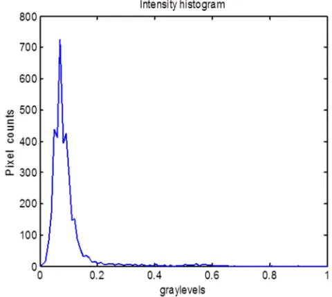
There are various types of features that can be extracted from the CT emphysema images for the multi-fractal analysis of emphysema patterns. In order to obtain feature descriptors with a very high discriminating power, this section considers the combinations of some of the important histogram features and the multi-fractal spectrum features for efficient classification of the emphysema patterns. The first histogram features are derived from the intensity histogram. An intensity histogram is a diagram in the form of a graph, plotting the number of pixels (fractional area) with a specific gray level versus the gray level value. It can be used for adjusting the brightness and contrast levels of the image. The shape of the histogram broadly describes the intensity distributions in the image. In some cases, a histogram may be scaled for adjusting the intensity levels or the contrast (e.g. histogram equalization). An example illustrating the
intensity histogram of an emphysema CT image is presented in Figure 1.
Figure 1. Intensity histogram of emphysema image.
The useful features that can be derived from the intensity histogram are the minimum and maximum values on the x-axis, and the maximum of the histogram on the y-axis.
3.1. Histograms of Emphysema Image
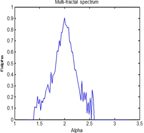
An α image is a matrix of the same dimension M x N as the original image but filled with α-values, with one-one corresponding to image pixels. Further information on the computation of alpha image can be found in the previous work [4, 7-8, 30-31]. An alpha-histogram of an image is therefore constructed using the α (m, n) values of the image as the pixel intensity values. As an example, an alpha-histogram of an emphysema image class is presented in Figure 2. Alpha-histogram can also be used as a global descriptor of intensity values, just like the intensity histogram.
Figure 2. Illustrating an example of alpha-histogram of emphysema image.
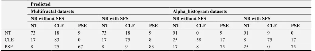
multi-fractal spectrum provides several shapes that could give more useful information to describe the characteristic properties of the images than the alpha-histogram.
Figure 3. Multi-fractal spectrum of an emphysema image sample.
Multi-fractal spectrum contains additional global information derived from the statistical self-similarity properties of the image at various scales to provide a global descriptor of the images. It generally has a higher
discriminating power compared to intensity and the alpha-histograms. Furthermore, it can also be observed from the analyses that the combination of the features extracted from the histograms and the multi-fractal spectrum could generate a descriptor with a better discriminating power. The multi-fractal spectrum of the same emphysema image used in Figure 2 is presented in Figure 3.
There is the possibility of improving the classification accuracy of the emphysema images by cascading the results obtained from the alpha-histogram with the multi-fractal spectrum since the new descriptor will definitely provide solutions to some of the limitations of the alpha-histogram and the multi-fractal spectrum. The newly constructed descriptor would combine the characteristic features of the multi-fractal spectra and that of the histograms, which makes it more superior and discriminating for efficient and accurate classification. There are some features that are very useful in a multi-fractal spectrum but are lacking in the histograms and vice versa.
3.2. Feature Selection Approach
The system overview for the classification approach involving several stages is presented in Figure 4. The features extracted from the descriptors are used as the input features for the FS algorithm. The two popular classifiers used in this study are trained on the outputs obtained from the FS as presented in Figure 4.
Figure 4. System overview of classification approach in emphysema images.
FS is an important part of pre-processing data in machine learning as the selection of important features can make the training phase to be less time consuming. This can be done by reducing the dimensions of data and thereby making the classifier algorithms to operate faster [29]. FSS is a mapping from a m-dimensional feature space (input space) to n-dimensional feature space (output), which can be represented as follows:
&'': )*+,→ )*+%, (1)
where m > n, RrXm is the matrix of the original data set with r instances or observations, RrXn is the reduced feature set containing r observations in the subset selection. It is also a technique of selecting only the predictor variables, that provide the best predictive power by simplifying and improving the model interpretation.
features in a data set by sequentially selecting the features until there is no further improvement in prediction accuracy. The important stages of the SFS algorithm are shown in Figure 5.
Most selection search approaches iteratively evaluate a subset of features, then modifies the subset and evaluates if the new subset is an improvement over the previous. Evaluation of the subsets requires a scoring metric that grades a subset of features. In this study, a function handle is used to define a criterion to determine the relevant features to be selected. Dimensionality reduction is achieved by calculating an optimal subset of predictive features of the original data. The algorithm automatically stops when further selection of feature subset has no effect on the classification errors.
Figure 5. Sequential forward selection method.
4. Results and Discussion
This section provides an outline of the experimental results obtained using images from the emphysema database [3], based on the implementation of the methods previously discussed. The feature vectors extracted from the multi-fractal spectra and the alpha-histograms have been used for classification and retrieving purposes. The histogram descriptors used for the classification experiment are constructed by dividing the range of α-values generated from the Holder exponent into 100 intervals. The alpha-histogram has been calculated for each alpha bin as the number of pixel counts with the α values within the α-range [α , α ]. The average of the alpha-histogram for four randomly selected images has been calculated and used as the feature vectors. In
the classification process of the NB classifier, the holdout partition method has been applied to divide the observations into training sets and test sets.
There is a scalar specifying the proportion of the number of observations to be randomly selected for validation. In order to achieve promising results since the accuracy of the classifiers depends on the training data; this scalar automatically selects 70 percent of the feature vectors for the training and 30 percent for testing. The performance of the classifiers is evaluated in the form of confusion matrix. A confusion matrix can be represented as a matrix M ∊ RkXk, a square matrix whose diagonal elements represents the actual classification accuracy where k is the number of classes in the data set. The classification error of the classifiers can be calculated as follows:
Error = 1 – 01 23 45 678 5 9 01
87 45 678 5 9 01 , (2)
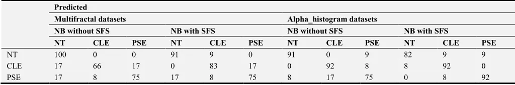
where trace (.) is the sum of all the elements in the diagonal, and sum (.) is the sum of all the entries in the confusion matrix. The feature vectors from the data sets are also trained with the BT classifier and the performances of the classification algorithms are examined with different experimental settings. A dimensionality reduction step has been implemented due to the presence of large irrelevant features in the data sets. The classification results obtained before and after the feature reduction for the NB classifier are presented in Table 1 in the form of confusion matrices.
The feature techniques reduced the feature variables in each data set to a set of feature variables with the highest discriminating power, such that the classifiers can be trained with the newly selected features by the SFS method. The performance of the classification system is measured by the classification accuracy generated by the confusion matrices.
The results obtained by the SFS achieve better dimensionality reductions and increase in learning accuracy by simplifying the model complexity. In Table 1, the classification accuracy of the multi-fractal datasets using the NB algorithm, increases from 74.3% before the FS to 77.6% after the FS and in the alpha-histogram dataset, the accuracy increases from 74.6% before the FS to 80.3% after the FS. The summary of the classification results produced by the BT algorithm before and after the FS is shown in Table 2.
Furthermore, the BT classifier outperformed the NB in multi-fractal datasets before and after the FS techniques, but the overall classification remains the same after the FS in the alpha-histogram data set.
Table 1. Naïve Bayes (NB) classification results with and without feature reductions.
Predicted
Multifractal datasets Alpha_histogram datasets
NB without SFS NB with SFS NB without SFS NB with SFS
NT CLE PSE NT CLE PSE NT CLE PSE NT CLE PSE
NT 73 18 9 73 18 9 91 0 9 91 9 0
CLE 17 83 0 17 75 8 25 58 17 8 75 17
The reason for the improvement in the performance of the algorithms after the FS in the data sets can be traced to the reduction in the complexity of the models, as complex models sometimes overfit the data and generate additional errors. Simplifying the complex models that would include the feature variables that are uncorrelated with one another would always reduce the computational complexity, which
might increase the accuracy. The difference in classification accuracy between the NB classifier and the BT over the multi-fractal datasets is 5.7% after the FS, while in alpha-histogram datasets, the overall classification remains the same after the FS but slightly higher before the FS (Tables 1 and 2).
Table 2. Bagged decision tree classification results with and without feature reductions.
Predicted
Multifractal datasets Alpha_histogram datasets
NB without SFS NB with SFS NB without SFS NB with SFS
NT CLE PSE NT CLE PSE NT CLE PSE NT CLE PSE
NT 82 9 9 91 0 9 81 19 0 91 9 0
CLE 8 75 17 25 67 8 0 75 25 0 75 25
PSE 0 17 83 8 0 92 0 25 75 17 8 75
The second approach is the concatenation of the relevant features obtained from the multi-fractal datasets and the alpha-histograms descriptors to generate new feature vectors. This is very easy since they both have the same number of rows and columns in dimension. Only the features selected by the FS technique have been used and the experimental results are presented in Table 3. The results in Table 3 reveal that this approach outperformed the results obtained in Tables 1 and 2. Significant improvements over the combined feature sets for the two classifier algorithms can be achieved after the FS. The difference in classification accuracy between the combined feature sets and the alpha-histogram datasets
(Table 3) for the NB classifier is about 3%, while the accuracy over the multi-fractal datasets for the BT increases by 5.3% after the FS.
Also in Table 3, the classification results of the combined features using the NB algorithm completely classified the normal emphysema images from the other pathological cases (CLE and PSE). The reasons for this improvement is due to the combination of the important feature variables with high discriminative power from both datasets since the irrelevant features have been filtered out by the FS methods. However, this approach consumes more processing time as the size of the dataset increases and thus reduces the computational speed.
Table 3. Classification results with and without feature selections for combined features.
Predicted
Multifractal datasets Alpha_histogram datasets
NB without SFS NB with SFS NB without SFS NB with SFS
NT CLE PSE NT CLE PSE NT CLE PSE NT CLE PSE
NT 100 0 0 91 9 0 91 0 9 82 9 9
CLE 17 66 17 0 83 17 0 92 8 8 92 0
PSE 17 8 75 17 8 75 8 17 75 0 8 92
Furthermore, the pairwise t-test of the classification results before and after the feature selection were carried out in order to determine whether the differences in accuracy are statistically significant or not. The t-test results of the classification results of the combined features in Table 3 are shown in equation (3); h = 0 indicates a failure to reject the null hypothesis.
h = 0, p-value = 0.7165, ci = -27.0733, 20.4067 (3)
This means the improvement achieved in the classification results is not statistically significant even at the 5% significant level. The same procedures are repeated for the previous results in Tables 1 and 2 before and after the feature selection in the multi-fractal and alpha-histogram data sets; the statistical results showed that the increase in the classification accuracy is not statistically significant since it failed to reject the null hypothesis at the 5% significant level. Another evidence to prove the statistical results is that the probability of observing a
value of the test statistic, as indicated by the p values, is far greater than the α-value of 0.05. Additionally, the 95% confidence interval on the mean of the difference does contain zero in all the results as can be seen in equation (3). These evidences are enough reasons to conclude that none of the classification results presented in this section is statistically significant at the α = 0.05 significant level.
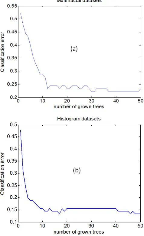
number of grown trees ranges from 20 to 40, and the performance of the algorithm is consistent. In order to fully
optimize the performance of the classifier, the number of grown trees used for both datasets is therefore 40.
Figure 6. Illustrating the variations between the classification error and the grown trees for bagged decision. (a) Multi-fractal datasets (b) Alpha-histogram datasets.
Ensemble of decision trees, particularly the BT has a way of estimating the predictor importance. Measure of importance for each predictor variable can be achieved by evaluating the effect on the classification margin if the values of the variable are permuted across the out-of-bag observations.
In other words, permuting a particular feature variable may either increase or decrease the classification accuracy. Figure 7 presents the results of the feature importance variables for the BT in each dataset. In the experiments, a threshold has been set to filter out those features whose ranking values are less than the required value; the features with the ranking values above this threshold value have been used for the classification process (Figure 7). In this case, the threshold has been reset to 0.42 in order to remove the unwanted features that could reduce the classification accuracy. The experimental results after removing the features below the threshold level as in Figure 7 reflect that the chosen features
have greater predictive power than all features as the classification accuracy further increases in multi-fractal and alpha-histogram features.
Multi-fractal Features
Alpha-histogram Features
Figure 7. Showing the ranking values of each feature variable in the datasets for multi-fractal and alpha-histogram features.
This improvement in the classification accuracy indicates that many features in the datasets are highly correlated and many are not strongly relevant. The FS ignored this set of data and only trained with the important features that would have significant impact on the overall accuracy.
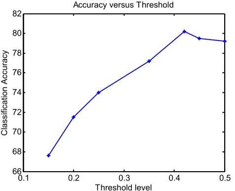
The performances of different threshold levels are tested on the overall classification accuracies. It was verified experimentally that the larger the threshold value the more important the selected predictor variables (Figure 8). For instance, the threshold value of 0.42 over the combined feature sets gives the highest classification accuracy while the threshold value below this level reduces the classification accuracy (Figure 8).
model that could generate more classification errors and thus reduces the classification accuracy. However, further increase in the threshold values beyond 0.42 does not have any significant improvement in the accuracy. The plot of the test accuracy demonstrating the effect of the threshold level on the overall classification accuracy is presented in Figure 8.
Figure 8. A graph of classification accuracy versus threshold level. Changes in the threshold level increase the accuracy until the peak value.
5. Conclusion
This paper has presented a novel approach for improving the classification accuracy of emphysema images by employing the FS techniques. The FS approach has been implemented to remove irrelevant features in the emphysema CT images. The two machine learning algorithms considered in this study; the NB and BT performed well on the datasets used. The results achieved by the classifiers are compared, the performance of the BT has been slightly better than the NB algorithms.
The experimental results also confirmed that multi-fractal descriptors could be used for the analysis and classification of emphysema in CT images. The information from the alpha-histogram descriptors has been very useful as the combination of the relevant features in the form of hybrid for both descriptors improved the classification accuracy. During the implementation of the BT, some of the important parameters that could be used to evaluate the performance of the classification system are presented.
The experimental results proved that the number of growing trees and the threshold values could affect the classification accuracy. Overall, the performance of the classifiers after FS has been consistently higher than the results without FS. Further research work might be to cascade the two classifier algorithms together over the combined feature sets or other medical data sets. This cascaded technique can be used to construct a new descriptor with a very powerful feature to improve the existing results. The performance of the classifiers can also be improved by parallelizing the algorithms using the GPU parallel computing as this might
improve the computational efficiency. In the future, other classification approach such as the local binary patterns (LBP) could also be implemented for further analysis of the emphysema images, and the results will be evaluated against the multi-fractal analysis.
Acknowledgements
The authors would like to sincerely thank Associate Professor Mukundan, Department of Computer Science and Software Engineering at the University of Canterbury for his substantial contributions towards this study.
References
[1] Y. Han, K. Park, & Y. K. Lee, “Confident wrapper-type semi-supervised feature selection using an ensemble classifier”. 2nd International Conference on Artificial Intelligence, Management Science and Electronic Commerce, AIMSEC – Proceedings.; pp. 4581–4586, 2011.
doi:10.1109/AIMSEC.2011.6010202.
[2] D. Wang, F. Nie, & H. Huang, “Feature Selection via Global Redundancy Minimization,” 2015; 4347 (c), pp. 1–14, 2015. doi:10.1109/TKDE.2015.2426703.
[3] L. Sørensen, S. B. Shaker, and M. De. Bruijne, “Quantitative Analysis of Pulmonary Emphysema using Local Binary Patterns,” IEEE transactions on medical imaging. 29, 2, pp. 559–569, 2010. [4] Ibrahim, M. and Mukundan, R. “Multi-fractal Techniques for Emphysema Classification in Lung Tissue Images”. Proceeding of International Conference on Environment, Chemistry and Biology; pp. 115-119, 2014.
[5] R. Duda, P. Hart, and D. Stork, “Pattern classification and scene analysis”. New York. 2011.
[6] A. Papadopoulos, M. Plissiti, and D. Fotiadis, “Medical-image processing and analysis for CAD systems”. Journal of Applied Signal Processing. 2, 5, pp. 25–41, 2005.
[7] M. Ibrahim & R. Mukundan, “Cascaded techniques for improving emphysema classification in computed tomography images,” Artificial Intelligence Research; 4 (2), pp. 112–118, 2015. doi:10.5430/air.v4n2p112.
[8] M. Ibrahim, “Multifractal Techniques for Analysis and Classification of Emphysema Images (PhD thesis),” University of Canterbury, 2017, http://hdl.handle.net/10092/14383. [9] J. W. Xu, & K. Suzuki, “Max-AUC feature selection in
computer-aided detection of polyps in CT colonography”. IEEE Journal of Biomedical and Health Informatics. 18 (2), pp. 585–593, 2014 doi:10.1109/JBHI.2013.2278023.
[10] H. Zhang, “A Novel Bayes Model: Hidden Naive Bayes. IEEE Transactions on Knowledge and Data Engineering,” 21 (10), pp. 1361–1371; 2009.
[11] Q. Liu, S. Shi, H. Zhu, & J. Xiao, “A Mutual
Information-Based Hybrid Feature Selection Method for Software Cost Estimation Using Feature Clustering”. 2014 IEEE 38th Annual Computer Software and Applications Conference. pp. 27–32, 2014;
doi:10.1109/COMPSAC.2014.99.
0.1 0.2 0.3 0.4 0.5
66 68 70 72 74 76 78 80 82
Accuracy versus Threshold
[12] J. A. Mangai, J Nayak, and V. S. Kumar, “A Novel Approach for Classifying Medical Images Using Data Mining Techniques”. International Journal of Computer Science and Electronics Engineering (IJCSEE). 2013; 1, 2.
[13] R. Bhuvaneswari, & K. Kalaiselvi, “Naive Bayesian Classification Approach in Healthcare Applications”. International Journal of Computer Science. 3 (1), pp. 106–112, 2012.
[14] H. Zhang, H. and J. Su, “Naive Bayes for optimal ranking. Journal of Experimental & Theoretical Artificial Intelligence”. 20, 2, pp. 79–93; 2008.
[15] L. M. Wang, X. L. Li, C. H. Cao, and S. M. Yuan,. “Combining decision tree and Naive Bayes for classification. Knowledge-Based Systems”, 19, 7, pp. 511–515; 2006. [16] R. Kohavi, and H. John, “Artihficial Intelligence Wrappers for
feature subset selection”. Data Mining and Visualization Silicon Graphics. 97, 273–324; 2011.
[17] P. Domingos, “On the Optimality of the Simple Bayesian Classifier under Zero-One Loss”. 29, pp. 103–130; 1997. [18] A. L. Bluma, and P. Langley, “Artificial Intelligence Selection
of relevant features and examples in machine”. pp. 245–271, 1997.
[19] Y. Liu, J. Guo, & J. Lee. “Halftone Image Classification Using LMS Algorithm and Naive Bayes”. IEEE Transactions on Image Processing. 20 (10), pp. 2837–2847, 2011. doi:10.1109/TIP.2011.2136354.
[20] J. Demšar, G. Leban, and B. Zupan, “Freeviz-an intelligent visualization approach for class-labeled multidimensional data sets”. Proceedings of IDAMAP. 1, pp. 13–18; 2005.
[21] C. Supriyanto, N. Yusof & B. Nurhadiono, “Two-Level F eature S election for Naive B ayes with Kernel Density,” Estimation in Question Classification based on B loom’s Cognitive Levels. pp. 1–5; 2013.
[22] L. T. D. Ladha, “Feature Selection Methods and Algorithms”. International Journal of Computer Science and Engineering. 3 (5), pp. 1787–1797; 2011.
[23] V. Ruiz and S. Nasuto, “Biomedical-image classification methods and techniques”. Costaridou, L. (ed.), 2005.
[24] H. A. Zhang, “A Novel Bayes Model: Hidden Naive Bayes”. IEEE Transactions on Knowledge and Data Engineering. 21, 10, pp. 1361–1371; 2009.
[25] K. Mikolajczyk, & C. Schmid, “Performance evaluation of local descriptors. IEEE Transactions on Pattern Analysis and Machine Intelligence,” 27 (10), 1615–30; 2005. doi:10.1109/TPAMI.2005.188.
[26] G. Zhao & P. Matti,”Local Binary Patterns with an Application to Facial Expressions”. Pattern Analysis and Machine Intelligence, IEEE Transactions on. 2007; 29 (6), pp. 915–928. [27] S. Marsland, “Machine Learning: An Algorithm Perspective”.
(2nd ed.). USA: CRC Press, 2014.
[28] M. Kallergi, “Evaluation strategies for medical-image analysis and processing methodologies”. International Journal of Image Analysis and Processing Methodologies; 2, 5, pp. 75–91. [29] T. Randen, and J. H. Husoy, “Filtering for texture
classification”: a comparative study. IEEE Transactions on Pattern Analysis and Machine Intelligence. 1999; 21, 4, pp. 291–310; 2005.
[30] R. Mukundan and A. Hemsley, “A. Tissue Image Classification Using Multi-Fractal Spectra”. International Journal of Multimedia Data Engineering and Management. 1, 2, pp. 62– 75; 2010.