Worst-Case Analysis of Selective Sampling
for Linear Classification
Nicol`o Cesa-Bianchi [email protected]
DSI, Universit`a di Milano via Comelico, 39
20135 Milano, Italy
Claudio Gentile [email protected]
DICOM, Universit`a dell’Insubria via Mazzini, 5
21100 Varese, Italy
Luca Zaniboni [email protected]
DTI, Universit`a di Milano via Bramante, 65
26013 Crema, Italy
Editor: Manfred Warmuth
Abstract
A selective sampling algorithm is a learning algorithm for classification that, based on the past observed data, decides whether to ask the label of each new instance to be classified. In this pa-per, we introduce a general technique for turning linear-threshold classification algorithms from the general additive family into randomized selective sampling algorithms. For the most popular algorithms in this family we derive mistake bounds that hold for individual sequences of examples. These bounds show that our semi-supervised algorithms can achieve, on average, the same accu-racy as that of their fully supervised counterparts, but using fewer labels. Our theoretical results are corroborated by a number of experiments on real-world textual data. The outcome of these experiments is essentially predicted by our theoretical results: Our selective sampling algorithms tend to perform as well as the algorithms receiving the true label after each classification, while observing in practice substantially fewer labels.
Keywords: selective sampling, semi-supervised learning, on-line learning, kernel algorithms, linear-threshold classifiers
1. Introduction
A selective sampling algorithm (see, e.g., Cohn et al., 1990; Cesa-Bianchi et al., 2003; Freund et al., 1997) is a learning algorithm for classification that receives a sequence of unlabelled instances and decides whether to query the label of the current instance based on the past observed data. The idea is to let the algorithm determine which labels are most useful to its inference mechanism, and thus achieve a good classification performance while using fewer labels.
costly human expertise. For this reason, it is clearly important to devise learning algorithms having the ability to exploit the label information as much as possible. An additional motivation for using selective sampling arises from the widespread use of kernel-based algorithms (Vapnik, 1998; Cris-tianini and Shawe-Taylor, 2001; Sch¨olkopf and Smola, 2002). In this case, saving labels implies using fewer support vectors to represent the hypothesis, which in turn entails a more efficient use of the memory and a shorter running time in both training and test phases.
Many algorithms have been proposed in the literature to cope with the broad task of learning with partially labelled data, working under both probabilistic and worst-case assumptions for either on-line or batch settings. These range from active learning algorithms (Campbell et al., 2000; Tong and Koller, 2000), to the query-by-committee algorithm (Freund et al., 1997), to the adversarial “apple tasting” and label efficient algorithms investigated by Helmbold et al. (2000) and Helmbold and Panizza (1997), respectively. More recent work on this subject includes (Bordes et al., 2005; Dasgupta et al., 2005; Dekel et al., 2006).
In this paper we present a mistake bound analysis for selective sampling versions of Perceptron-like algorithms. In particular, we study the standard Perceptron algorithm (Rosenblatt, 1958; Block, 1962; Novikov, 1962) and the second-order Perceptron algorithm (Cesa-Bianchi et al., 2005). Then, we argue how to extend the above analysis to the general additive family of linear-threshold algo-rithms introduced by Grove et al. (2001) and Warmuth and Jagota (1997) (see also Cesa-Bianchi and Lugosi, 2003; Gentile, 2003; Gentile and Warmuth, 1999; Kivinen and Warmuth, 2001), and we provide details for a specific algorithm in this family, i.e., the (zero-threshold) Winnow algo-rithm (Littlestone, 1988, 1989; Grove et al., 2001).
Our selective sampling algorithms use a simple randomized rule to decide whether to query the label of the current instance. This rule prescribes that the label should be obtained with probability
b/(b+|bp|), wherep is the (signed) margin achieved by the current linear hypothesis on the currentb
instance, and b>0 is a parameter of the algorithm acting as a scaling factor on bp. Note that
a label is queried with a small probability whenever the margin bp is large in magnitude. If the
label is obtained, and it turns out that a mistake has been made, then the algorithm proceeds with its standard update rule. Otherwise, the algorithm’s current hypothesis is left unchanged. It is important to remark that in our model we evaluate algorithms by counting their prediction mistakes also on those time steps when the true labels remain unknown. For each of the algorithms we consider a bound is proven on the expected number of mistakes made in an arbitrary data sequence, where the expectation is with respect to the randomized sampling rule.
Our analysis reveals an interesting phenomenon. In all algorithms we analyze, a proper choice of the scaling factor b in the randomized rule yields the same mistake bound as the one achieved by the original algorithm before the introduction of the selective sampling mechanism. Hence, in some sense, our technique exploits the margin information to select those labels that can be ignored without increasing (in expectation) the overall number of mistakes.
One may suspect that this gain is not real: it might very well be the case that the tuning of b preserving the original mistake bound forces the algorithm to query all but an insignificant number of labels. In the last part of the paper we present some experiments contradicting this conjecture. In particular, by running our algorithms on real-world textual data, we show that no significant decrease in the predictive performance is suffered even when b is set to values that leave a significant fraction of the labels unobserved.
Perceptron-like selective sampling algorithms. In Section 3 we extend our margin-based argument to the zero-threshold Winnow algorithm. Empirical comparisons are reported in Section 4. Finally, Section 5 is devoted to conclusions and open problems.
Notation and basic definitions
Anexample is a pair(x,y), where x∈Rdis aninstance vector and y∈ {−1,+1}is the associated binary label.
We consider the following selective sampling variant of the standard on-line learning model (An-gluin, 1988; Littlestone, 1988). Learning proceeds in a sequence oftrials. In the generic trial t the algorithm observes instance xt, outputs a predictionybt ∈ {−1,+1}for the label yt associated with
xt, and decides whether or not to ask the label yt. No matter what the algorithm decides, we say that the algorithm has made aprediction mistake if byt 6=yt. We measure the performance of a linear-threshold algorithm by the total number of mistakes it makes on a sequence of examples (including the trials where the true label yt remains unknown). The goal of the algorithm is to bound, on an arbitrary sequence of examples, the amount by which this total number of mistakes exceeds the performance of the best linear predictor in hindsight.
In this paper we are concerned with selective sampling versions of linear-threshold algorithms. When run on a sequence (x1,y1),(x2,y2), . . . of examples, these algorithms compute a sequence
w0,w1, . . .of weight vectors wt ∈Rd, where wt can only depend on the past examples(x1,y1),. . ., (xt,yt) but not on the future ones, (xs,ys) for s>t. In each trial t=1,2, . . .the linear-threshold algorithm predicts yt using1ybt =SGN(bpt)where pbt =w⊤t−1xt is the margin of wt−1on the instance
xt. If the label yt is queried, then the algorithm (possibly) uses yt to compute a new weight wt; on the other hand, if yt remains unknown then wt =wt−1.
We identify an arbitrary linear-threshold classifier with its coefficient vector u∈Rd. For a fixed sequence(x1,y1), . . . ,(xn,yn)of examples and a given margin thresholdγ>0, we measure the performance of u by its cumulativehinge loss (Freund and Schapire, 1999; Gentile and Warmuth, 1999)
Lγ,n(u) = n
∑
t=1
ℓγ,t(u) = n
∑
t=1
(γ−ytu⊤xt)+
where we used the notation(x)+=max{0,x}. In words, the hinge loss, also calledsoft margin in
the statistical learning literature (Vapnik, 1998; Cristianini and Shawe-Taylor, 2001; Sch¨olkopf and Smola, 2002), measures the extent to which the hyperplane u separates the sequence of examples with margin at leastγ.
We represent the algorithm’s decision of querying the label at time t through the value of a Bernoulli random variable Zt, whose parameter is determined by the specific selection rule used by the algorithm under consideration. Though we make no assumptions on the source generating the sequence(x1,y1),(x2,y2), . . ., we require that each example(xt,yt) be generated before the value of Zt is drawn. In other words, the source cannot use the knowledge of Zt to determine xt and yt. We useEt−1[·]to denote the conditional expectationE[·|Z1, . . . ,Zt−1]and Mt to denote the indicator function of the eventybt6=yt, whereybt is the prediction at time t of the algorithm under consideration.
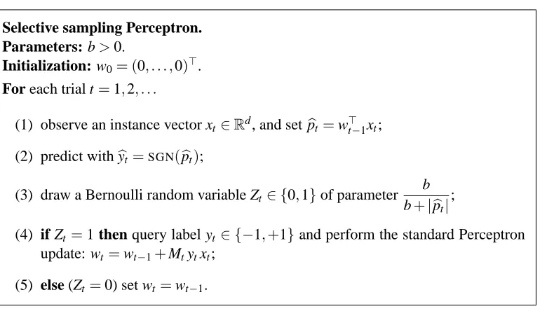
Selective sampling Perceptron. Parameters: b>0.
Initialization: w0= (0, . . . ,0)⊤. For each trial t=1,2, . . .
(1) observe an instance vector xt ∈Rd, and set bpt=w⊤t−1xt; (2) predict withbyt =SGN(pbt);
(3) draw a Bernoulli random variable Zt ∈ {0,1}of parameter
b b+|bpt|
;
(4) if Zt =1 then query label yt ∈ {−1,+1}and perform the standard Perceptron update: wt =wt−1+Mtytxt;
(5) else (Zt =0) set wt=wt−1.
Figure 1: A selective sampling version of the classical Perceptron algorithm.
Finally, whenever the distribution laws of Z1,Z2, . . .and M1,M2, . . .are clear from the context, we use the abbreviation
Lγ,n(u) =E "
n
∑
t=1
MtZtℓγ,t(u) #
.
Note that Lγ,n(u)≤Lγ,n(u)trivially holds for all choices ofγ, n, and u.
2. Selective Sampling Algorithms and Their Analysis
In this section we describe and analyze three algorithms: a selective sampling version of the clas-sical Perceptron algorithm (Rosenblatt, 1958; Block, 1962; Novikov, 1962), a variant of the same algorithm with a dynamically tuned parameter, and a selective sampling version of the second-order Perceptron algorithm (Cesa-Bianchi et al., 2005). It is worth pointing out that, like any Perceptron-like update rule, each of the algorithms presented in this section can be efficiently run in any given reproducing kernel Hilbert space once the update rule is expressed in an equivalent dual-variable form (see, e.g., Vapnik, 1998; Cristianini and Shawe-Taylor, 2001; Sch¨olkopf and Smola, 2002). Note that, in the case of kernel-based algorithms, label efficiency provides the additional benefit of a more compact representation of the trained classifiers. The experiments reported in Section 4 were indeed obtained using a dual-variable implementation of our algorithms.
2.1 Selective Sampling Perceptron
valuebpt=wt⊤−1xt. Then the algorithm decides whether to query the label yt through the randomized rule described in the introduction: a coin with bias b/(b+|pbt|)is flipped; if the coin turns up heads (Zt =1 in Figure 1), then the label yt is queried. If a prediction mistake is observed (byt 6=yt), then the algorithm updates vector wt according to the usual Perceptron additive rule. On the other hand, if either the coin turns up tails orbyt =yt (Mt=0 in Figure 1), then no update takes place.
The following theorem shows that our selective sampling Perceptron can achieve, in expectation, the same mistake bound as the standard Perceptron’s, but using fewer labels.
Theorem 1 If the algorithm of Figure 1 is run with input parameter b>0 on a sequence(x1,y1), (x2,y2),. . .∈Rd× {−1,+1}of examples, then for all n≥1, all u∈Rd, and allγ>0,
E
" n
∑
t=1
Mt #
≤
1+X
2 2b
Lγ,n(u)
γ +k
uk2 2b+X22
8 bγ2
where X =maxt=1,...,nkxtk. Furthermore, the expected number of labels queried by the algorithm
equals∑nt=1Ehb+b|bpt|i.
The above bound depends on the choice of parameter b. In general, b might be viewed as a noise parameter ruling the extent to which a linear threshold model fits the data at hand. In principle, the optimal tuning of b is easily computed. Choosing
b= X
2 2
s
1+ 4γ 2
||u||2X2
Lγ,n(u)
γ
in Theorem 1 gives the following bound on the expected number of mistakes
Lγ,n(u)
γ +k
uk2X2
2γ2 +
kukX
γ
s
Lγ,n(u)
γ +k
uk2X2
4γ2 . (1)
This is an expectation version of the mistake bound for the standard Perceptron algorithm (Freund and Schapire, 1999; Gentile, 2003; Gentile and Warmuth, 1999). Note that in the special case when the data are linearly separable with marginγ∗the optimal tuning simplifies to b=X2/2 and yields the familiar Perceptron bound kukX2/(γ∗)2. Hence, in the separable case, we obtain the somewhat counterintuitive result that the standard Perceptron bound is achieved by an algorithm whose label rate does not (directly) depend on how big the separation margin is.
All of the above shortcomings will be fixed in Section 2.2, where we present an adaptive pa-rameter version of the algorithm in Figure 1. Via a more involved analysis, we show that it is still possible to achieve a bound having the same form as (1) with no prior information.
That said, we are ready to prove Theorem 1.
Proof of Theorem 1. The proof extends the standard proof of the Perceptron mistake bound (see, e.g., Duda et al., 2000, Chap. 5) which is based on estimating the influence of an update on the distanceku−wt−1k2 between the current weight vector wt−1 and an arbitrary “target” hyperplane
u. Our analysis uses a tighter estimate on this influence, and then uses a probabilistic analysis to
turn this increased tightness into an expected saving on the number of observed labels. Since this probabilistic analysis only involves the terms that are brought about by the improved estimate, we are still able to recover (in expectation) the original Perceptron bound.
Fix an arbitrary sequence(x1,y1), . . . ,(xn,yn)∈Rd× {−1,+1}of examples. Let t be an update trial, i.e., a trial such that MtZt =1. We can write
γ−ℓγ,t(u) = γ−(γ−ytu⊤xt)+
≤ ytu⊤xt
= yt(u−wt−1+wt−1)⊤xt = ytw⊤t−1xt+
1
2ku−wt−1k 2
−12ku−wtk2+ 1
2kwt−1−wtk 2 = ytpbt+
1
2ku−wt−1k 2
−12ku−wtk2+ 1
2kwt−1−wtk 2 .
Since the above inequality holds for anyγ>0 and any u∈Rd, we can replaceγbyαγand u byαu,
whereαis a constant to be optimized.
Rearranging, and using ytbpt≤0 implied by Mt=1, yields
αγ+|pbt| ≤αℓγ,t(u) + 1
2kαu−wt−1k 2
−12kαu−wtk2+ 1
2kwt−1−wtk 2
.
Note that, instead of discarding the term|bpt|, as in the original Perceptron proof, we keep it around. This yields a stronger inequality which, as we will see, is the key to achieving our final result.
If t is such that MtZt =0 then no update occurs and wt=wt−1. Hence we conclude that, for any trial t,
MtZt(αγ+|bpt|)≤MtZtαℓγ,t(u)
+1
2kαu−wt−1k 2
−12kαu−wtk2+
MtZt
2 kwt−1−wtk 2
. (2)
We now sum the above over t, usekwt−1−wtk2≤X2and recall that w0=0. We get n
∑
t=1
MtZt
αγ+|bpt| −
X2
2
≤α n
∑
t=1
MtZtℓγ,t(u) +
α2 2 kuk
2
.
Now chooseα= (2b+X2)/(2γ), where b>0 is the algorithm’s parameter. The above then becomes n
∑
t=1
MtZt b+|bpt|≤
2b+X2
2γ n
∑
t=1
MtZtℓγ,t(u) +k
uk2 2b+X22
A similar inequality is also obtained in the analysis of the standard Perceptron algorithm. Here, however, we have added the random variable Zt, associated with the selective sampling, and kept the term|bpt|. Note that this term also appears in the conditional expectation of Zt, since we have definedEt−1Ztas b/(b+|bpt|). This fact is exploited now, when we take expectations on both sides of (3). On the left-hand side we obtain
E
" n
∑
t=1
MtZt b+|bpt| #
=E
" n
∑
t=1
Mt b+|pbt|
Et−1Zt #
=E
" n
∑
t=1
b Mt #
,
where the first equality is proven by observing that Mt and pbt are determined by Z1, . . . ,Zt−1(that is, they are both measurable with respect to theσ-algebra generated by Z1, . . . ,Zt−1). Dividing by b we obtain the claimed inequality on the expected number of mistakes.
The value ofE[∑tn=1Zt](the expected number of queried labels) trivially follows from
E
" n
∑
t=1
Zt #
=E
" n
∑
t=1
Et−1Zt #
.
This concludes the proof.
2.2 Selective Sampling Perceptron: Adaptive Version
In this section we show how to learn the best trade-off parameter b in an on-line fashion. Our goal is to devise a time-changing expression for this parameter that achieves a bound on the expected number of mistakes having the same form as (1)—i.e., with constant 1 in front of the cumulative hinge loss term—but relying on no prior knowledge whatsoever on the sequence of examples.
We follow the “self-confident” approach introduced by Auer et al. (2002) and Gentile (2001) though, as pointed out later, our self-confidence tuning here is technically different, since it does not rely on projections to control the norm of the weight (as in, e.g., Herbster and Warmuth, 2001; Auer et al., 2002; Gentile, 2001, 2003).
Our adaptive version of the selective sampling Perceptron algorithm is described in Figure 2. The algorithm still has a parameter β>0 but, as we will see, any constant value for β leads to bounds of the form (1). Thusβ has far less influence on the final bound than the b parameter in Figure 1.
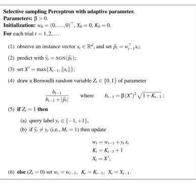
The adaptive algorithm is essentially the same as the one in Figure 1, but for maintaining two further variables, Xtand Kt. At the end of trial t, variable Xt stores the maximal norm of the instance vectors involved in updates up to and including time t, while Kt just counts the number of such updates. Observe that bt increases with (the square root of) this number, thereby implementing the easy intuition that the more updates are made by the algorithm the harder the problem looks, and the more labels are needed on average. However the reader should not conclude from this observation that the label rate bt−1/(bt−1+|pbt|)converges to 1 as t→∞, since btdoes not scale with time t but with the number of updates made up to time t, which can be far smaller than t. At the same time, the margin|pbt|might have an erratic behavior whose oscillations can also grow with the number of updates.
Selective sampling Perceptron with adaptive parameter. Parameters: β>0.
Initialization: w0= (0, . . . ,0)⊤, X0=0, K0=0. For each trial t=1,2, . . .
(1) observe an instance vector xt ∈Rd, and set bpt=w⊤t−1xt; (2) predict withbyt =SGN(pbt);
(3) set X′=max{Xt−1,kxtk};
(4) draw a Bernoulli random variable Zt ∈ {0,1}of parameter
bt−1
bt−1+|pbt|
where bt−1=β(X′)2 p
1+Kt−1; (5) if Zt =1 then
(a) query label yt∈ {−1,+1},
(b) ifybt 6=yt (i.e., Mt =1) then update
wt=wt−1+ytxt
Kt =Kt−1+1
Xt =X′;
(6) else (Zt =0) set wt=wt−1, Kt=Kt−1, Xt =Xt−1.
Figure 2: Adaptive parameter version of the selective sampling Perceptron algorithm.
Theorem 2 If the algorithm of Figure 2 is run with input parameterβ>0 on a sequence(x1,y1), (x2,y2). . .∈Rd× {−1,+1}of examples, then for all n≥1, all u∈Rd, and allγ>0,
E
" n
∑
t=1
Mt #
≤Lγ,nγ(u)+ R 2β+
B2
2 +B s
Lγ,n(u)
γ +
R
2β+
B2 4
where
B=R+1+3R/2
β and R=k
uk maxt=1,...,nkxtk
γ .
Moreover, the expected number of labels queried by the algorithm equals∑nt=1Eh bt−1
bt−1+|bpt|
i
.
bound (unlike the one in Theorem 1) becomes the Perceptron bound, as given by Gentile (2003). Clearly, the larger isβthe more labels are queried on average over the trials. Thusβhas also an indirect influence on the hinge loss term Lγ,n(u). In particular, we might expect that a small value ofβmakes the number of updates shrink (note that in the limit whenβ→0 this number goes to 0). Proof of Theorem 2. Fix an arbitrary sequence(x1,y1), . . . ,(xn,yn)∈Rd× {−1,+1}of examples and let X =maxt=1,...,nkxtk. The proof is a more involved version of the proof of Theorem 1. We start from the one-trial equation (2) established there, where we replace the (constant) stretching factorα by the time-varying factor ct−1/γ, where ct−1≥0 will be set later and γ>0 is the free margin parameter of the hinge loss. This yields
MtZt(ct−1+|pbt|)≤MtZt
ct−1
γ ℓγ,t(u)
+1 2
ct−1
γ u−wt−1 2
−12
ct−1
γ u−wt 2
+MtZt
2 kwt−1−wtk 2
.
From the update rule in Figure 2 we have(MtZt/2)kwt−1−wtk2 ≤(MtZt/2)kxtk2. We rearrange and divide by bt−1. This yields
MtZt
ct−1+|bpt| − kxtk2/2
bt−1
!
≤MtZt
ct−1
bt−1
ℓγ,t(u)
γ
+ 1 2 bt−1
ct−1
γ u−wt−1 2 −
ct−1
γ u−wt 2! . (4)
We now transform the difference of squared norms in (4) into a pair of telescoping differences, 1
2 bt−1
ct−1
γ u−wt−1 2 −
ct−1
γ u−wt 2! = 1 2 bt−1
ct−1
γ u−wt−1 2 − 1
2 bt
ct
γu−wt 2 + 1 2 bt
ct
γu−wt 2
−2 b1 t−1
ct−1
γ u−wt 2 . (5)
If we set
ct−1= 1
2 max{Xt−1,kxtk} 2
+bt−1 we can expand the difference of norms (5) as follows
(5) =kuk 2 2γ2
c2t
bt −
c2t−1 bt−1
!
+u⊤wt
γ
ct−1
bt−1−
ct
bt
+kwtk 2 2
1
bt − 1
bt−1
≤kuk
2 2γ2
c2t
bt −
c2t−1 bt−1
!
+kukkwtk
γ
ct−1
bt−1−
ct
bt
(6)
where in the last step we used bt ≥bt−1and the inequality
ct−1
bt−1 ≥
ct
which follows from ct−1/bt−1=1
2β√1+Kt−1
+1.
Recall now the standard way of bounding the norm of a Perceptron weight vector in terms of the number of updates,
kwtk2 = kwt−1k2+MtZtytwt⊤−1xt+MtZtkxtk2 ≤ kwt−1k2+MtZtkxtk2
≤ kwt−1k2+MtZtX2 which, combined with w0=0, implies
kwtk ≤X √
Kt for any t. (7)
Applying inequality (7) to (6) yields
(5)≤kuk 2 2γ2
c2t bt −
ct2−1 bt−1
!
+kukX
√
Kt
γ
ct−1
bt−1−
ct
bt
. (8)
We continue by bounding from above the last term in (8). If t is such that MtZt =1 we have
Kt =Kt−1+1. Thus we can write
√
Kt
ct−1
bt−1−
ct bt = √ Kt 2β 1 √
1+Kt−1− 1
√
1+Kt = √ Kt 2β 1 √
Kt −
1
√
1+Kt
= 1 2β
√
1+Kt−√Kt √
1+Kt
≤ 1
4β
1
√
Kt√1+Kt
(using√1+x−√x≤ 2√1 x) ≤ 1 4β 1 Kt .
On the other hand, if MtZt =0 we have bt=bt−1and ct =ct−1. Hence, for any trial t we obtain
√
Kt
ct−1
bt−1−
ct
bt
≤M4tβZt K1 t
.
Putting together as in (4) and using ct−1− kxtk2/2≥bt−1on the left-hand side yields
MtZt
bt−1+|bpt|
bt−1
≤MtZt
ct−1
bt−1
ℓγ,t(u)
γ
+ 1 2bt−1
ct−1
γ u−wt−1 2 − 1 2bt ct
γu−wt 2
+kuk 2 2γ2
c2t
bt −
c2t−1 bt−1
!
+kukX
γ
MtZt 4β
1
holding for any trial t, any u∈Rd, and anyγ>0.
Now, as in the proof of Theorem 1, we sum over t=1, . . . ,n, use w0=0, and simplify n
∑
t=1
MtZt
bt−1+|bpt|
bt−1 !
≤ 1γ n
∑
t=1
MtZt
ct−1
bt−1
ℓγ,t(u) (9)
+ c 2 n
bn kuk2
2γ2 − 1 2 bn
cn
γu−wn 2 (10) + 1 4β
kukX
γ
n
∑
t=1
MtZt
Kt
.
We now proceed by bounding separately the terms in the right-hand side of the above inequality. For (9) we get
1
γ
ct−1
bt−1
ℓγ,t(u) = 1
γ
1 2β√1+Kt−1
+1
ℓγ,t(u)
≤ 1γ 1
2β√1+Kt−1
γ+kukX+ℓγ,t(u)
γ
(sinceℓγ,t(u)≤γ+kukX ) = 1
2β
1+kukX
γ
1
√
1+Kt−1
+ℓγ,t(u)
γ .
For (10) we obtain
c2n bn
kuk2
2γ2 − 1 2bn cn
γu−wn 2
= cn
bn
u⊤wn
γ −k
wnk2 2bn ≤ bcn
n
u⊤wn
γ
≤ cn
bn
kuk kwnk
γ
≤
1+ 1 2β√1+Kn
kukX√Kn
γ
where in the last step we used (7). Using these expressions to bound the left-hand side of (9) yields n
∑
t=1
MtZt
bt−1+|pbt|
bt−1 !
≤1γ n
∑
t=1
MtZtℓγ,t(u) + 1 2β
1+kukX
γ
n
∑
t=1
MtZt √
1+Kt−1
(11)
+
1+ 1 2β√1+Kn
kukX√Kn
γ +
1 4β
kukX
γ
n
∑
t=1
MtZt
Kt
. (12)
Next, we focus on the second sum in (11) and the sum in (12). Since MtZt=1 implies Kt=Kt−1+1 we can write
n
∑
t=1
MtZt √
1+Kt−1
=
∑
t : MtZt=1
1 √ Kt = Kn
∑
t=1 1
√
t ≤2
√
Similarly for the other sum, but using a more crude bound, n
∑
t=1
MtZt
Kt
=
∑
t : MtZt=1
1
Kt ≤t : M
∑
tZt=1 1√
Kt ≤
2√Kn.
Recalling the short-hand R= (kukX)/γ, we apply these bounds to (11) and (12). After a simple overapproximation this gives
n
∑
t=1
MtZt
bt−1+|pbt|
bt−1 !
≤1γ n
∑
t=1
MtZtℓγ,t(u) + √
Kn
R+1+3R/2
β
+ R
2β .
We are now ready to take expectations on both sides. As in the proof of Theorem 1, sinceEt−1Zt= bt−1
bt−1+|pbt|and both Mtand bt−1are measurable with respect to theσ-algebra generated by Z1, . . . ,Zt−1,
we obtain
E
" n
∑
t=1
MtZt
bt−1+|bpt|
bt−1 !#
=E
" n
∑
t=1
Mt #
.
In taking the expectation on the right-hand side, we first bound Kn=∑nt=1MtZt as Kn≤∑nt=1Mt, then exploit the concavity of the square root. This results in
n
∑
t=1
EMt ≤
Lγ,n(u)
γ +
R+1+3R/2
β
s n
∑
t=1
EMt+
R
2β .
Solving the above inequality for∑nt=1EMt gives the stated bound on the expected number of mis-takes.
Finally, as in the proof of Theorem 1, the expected number of labels queried by the algorithm trivially follows from
E
" n
∑
t=1
Zt #
=E
" n
∑
t=1
Et−1Zt #
concluding the proof.
The proof of Theorem 2 is reminiscent of the analysis of the “self-confident” dynamical tuning used in Auer et al. (2002) and Gentile (2001). In those papers, however, the variable learning rate was combined with a re-normalization step of the weight. Here we use a different technique based on a time-changing stretching factorαt−1=ct−1/γfor the comparison vector u. This alternative approach is made possible by the boundedness of the hinge loss terms, as shown by the inequality
ℓγ,t(u)≤γ+kukX .
2.3 Selective Sampling Second-Order Perceptron
We now consider a selective sampling version of the second-order Perceptron algorithm introduced by Cesa-Bianchi et al. (2005). The second-order Perceptron algorithm might be seen as running the standard (first-order) Perceptron algorithm as a subroutine. Let vt−1 denote the weight vector computed by the standard Perceptron algorithm. In trial t, instead of using the sign of v⊤t−1xt to predict the current instance xt, the second-order algorithm predicts through the sign of the margin
b
pt = M−1/2vt−1
⊤ M−1/2x t
Here M=I+∑sxsxs⊤+xtxt⊤is a (full-rank) positive definite matrix, where I is the d×d identity matrix, and the sum∑sxsx⊤s runs over the mistaken trials s up to time t−1. If, when using the above prediction rule, the algorithm makes a mistake in trial t, then vt−1 is updated according to the standard Perceptron rule and t is included in the set of mistaken trials. Hence the second-order algorithm differs from the standard Perceptron algorithm in that, before each prediction, a linear transformation M−1/2is applied to both the current Perceptron weight vt−1and the current instance
xt. This linear transformation depends on the correlation matrix defined over mistaken instances, including the current one. As explained in Cesa-Bianchi et al. (2005), this linear transformation has the effect of reducing the number of mistakes whenever the instance correlation matrix∑sxsx⊤s +
xtx⊤t has a spectral structure that causes an eigenvector with small eigenvalue to correlate well with a good linear approximator u of the entire data sequence. In such situations, the mistake bound of the second-order Perceptron algorithm can be shown to be significantly better than the one for the first-order algorithm.
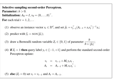
In what follows, we use At−1 to denote I+∑sxsx⊤s where the sum ranges over the mistaken trials between trial 1 and trial t−1. We derive a selective sampling version of the second-order algorithm in much the same way as we did for the standard Perceptron algorithm: The selective sampling second-order Perceptron algorithm predicts and then decides whether to ask for the label
yt using the same randomized rule as the one in Figure 1. In Figure 3 we provide a pseudo-code description and introduce the notation used in the analysis.
The analysis follows the same pattern as the proof of Theorem 1. A key step is a one-trial progress equation developed by Forster (1999) for a regression framework. See also Azoury and Warmuth (2001). As before, the comparison between the second-order Perceptron’s bound and the one contained in Theorem 3 reveals that the selective sampling algorithm can achieve, in expecta-tion, the same mistake bound using fewer labels.
Theorem 3 If the algorithm of Figure 3 is run with parameter b>0 on a sequence(x1,y1),(x2,y2),
. . .∈Rd× {−1,+1}of examples, then for all n≥1, all u∈Rd, and allγ>0,
E
" n
∑
t=1
Mt #
≤Lγ,nγ(u)+ b
2γ2u⊤E[An]u+ 1 2b
d
∑
i=1
Eln(1+λi)
whereλ1, . . . ,λd are the eigenvalues of the (random) correlation matrix ∑nt=1MtZtxtxt⊤ and An=
I+∑nt=1MtZtxtx⊤t (thus 1+λiis the i-th eigenvalue of An). Moreover, the expected number of labels
queried by the algorithm equals∑nt=1Ehb+b|pbt|i.
Again, the above bound depends on the algorithm’s parameter b. Setting
b=γ
s
∑d
i=1Eln(1+λi)
u⊤E[An]u
in Theorem 3 we are led to the bound
E
" n
∑
t=1
Mt #
≤Lγ,nγ(u)+1
γ
s
(u⊤E[An]u) d
∑
i=1
Eln(1+λi). (13)
Selective sampling second-order Perceptron. Parameter: b>0.
Initialization: A0=I, v0= (0, . . . ,0)⊤. For each trial t=1,2, . . .
(1) observe an instance vector xt ∈Rd, and set bpt=vt⊤−1(At−1+xtx⊤t )−1xt; (2) predict withbyt =SGN(pbt);
(3) draw a Bernoulli random variable Zt ∈ {0,1}of parameter
b b+|bpt|
;
(4) if Zt=1 then query label yt ∈ {−1,+1}and perform the standard second-order Perceptron update:
vt = vt−1+Mtytxt ,
At = At−1+Mtxtx⊤t ; (5) else (Zt =0) set vt=vt−1and At =At−1.
Figure 3: A selective sampling version of the second-order Perceptron algorithm.
bound might be sharper than its deterministic counterpart, since the magnitude of the three quan-tities Lγ,n(u), u⊤E[An]u, and∑di=1Eln(1+λi) is ruled by the size of the random set of updates
{t : MtZt =1}, which is typically smaller than the set of mistaken trials of the deterministic
algo-rithm.
However, as for the algorithm in Figure 1, this parameter tuning turns out to be unrealistic, since it requires preliminary information on the structure of the sequence of examples. Unlike the first-order algorithm, we have been unable to devise a meaningful adaptive parameter version for the algorithm in Figure 3.
Proof of Theorem 3. The proof proceeds along the same lines as the proof of Theorem 1, thus we only emphasize the main differences. In addition to the notation given there, we defineΦt to be the (random) function
Φt(u) = 1 2kuk
2+
∑
t s=1MsZs 2 (ys−u
⊤x s)2.
The quantityΦt(u), which is the regularized cumulative square loss of u on the past mistaken trials, plays a key role in the proof. Indeed, we now show that the algorithm incurs on each mistaken trial a square loss yt−bpt
2
When trial t is such that MtZt =1 we can exploit a result proven by Forster (1999) for lin-ear regression (proof of Theorem 3 therein), where it is essentially shown that choosing pbt =
v⊤t−1(At−1+xtxt⊤)−1xt (as in Figure 3) yields
1
2 bpt−yt 2
=inf
v Φt+1(v)−infv Φt(v) + 1 2x
⊤
t At−1xt− 1 2
xt⊤At−−11xt
b
p2t .
On the other hand, if trial t is such that MtZt =0 we have infv∈RdΦt+1(v) =infv∈RdΦt(v). Hence
the equality
MtZt
2 pbt−yt 2
=inf
v Φt+1(v)−infv Φt(v) +
MtZt 2 x
⊤
t A−t 1xt−
MtZt 2
x⊤t A−t−11xt
b
p2t
holds for all trials t. We drop the term−MtZt xt⊤A−t−11xt
b
p2t/2, which is nonpositive (since At−1is positive definite), and sum over t=1, . . . ,n. Observing that infvΦ1(v) =0, we obtain
1 2
n
∑
t=1
MtZt pbt−yt2 ≤ inf
v Φn+1(v)−infv Φ1(v) + 1 2
n
∑
t=1
MtZtx⊤t A−t 1xt
≤ Φn+1(u) +1
2 n
∑
t=1
MtZtx⊤t A−t 1xt ≤ 1
2kuk 2+1
2 n
∑
t=1
MtZt u⊤xt−yt 2
+1 2
n
∑
t=1
MtZtxt⊤A−t 1xt
holding for any u∈Rd.
Expanding the squares and performing trivial simplifications we arrive at the following inequal-ity
1 2
n
∑
t=1
MtZt pb2t −2ytpbt
≤ 12
"
kuk2+ n
∑
t=1
MtZt u⊤xt 2#
− n
∑
t=1
MtZtytu⊤xt+ 1 2
n
∑
t=1
MtZtx⊤t A−t 1xt . (14)
We focus on the right-hand side of (14). We rewrite the first term and bound from above the last term. For the first term we have
1 2
"
kuk2+ n
∑
t=1
MtZt u⊤xt2 #
=1 2u
⊤ I+
∑
nt=1
xtxt⊤MtZt !
u=1
2u ⊤A
For the third term, we use a property of the inverse matrices A−t 1 (see, e.g., Lai and Wei, 1982; Azoury and Warmuth, 2001; Forster, 1999; Cesa-Bianchi et al., 2005),
1 2
n
∑
t=1
MtZtx⊤t A−t 1xt = 1 2
n
∑
t=1
1−|At−1|
|At|
≤ 12 n
∑
t=1 ln |At|
|At−1| = 1
2ln
|An| |A0| = 1
2ln|An| = 1
2 d
∑
i=1
ln(1+λi)
where we recall that 1+λiis the i-th eigenvalue of An.
Replacing back, observing that −ytbpt ≤0 whenever Mt =1, dropping the term involving pb2t, and rearranging yields
n
∑
t=1
MtZt |bpt|+ytu⊤xt≤ 1 2u
⊤A nu+
1 2
d
∑
i=1
ln(1+λi).
At this point, as in the proof of Theorem 1, we introduce hinge loss terms and stretch the comparison vector u to bγu, where b is the algorithm’s parameter. We obtain
n
∑
t=1
MtZt |bpt|+b
≤bγ n
∑
t=1
MtZtℓγ,t(u) +
b2
2γ2u⊤Anu+ 1 2
d
∑
i=1
ln(1+λi).
We take expectations on both sides. Recalling thatEt−1Zt=b/(b+|bpt|), and proceeding similarly to the proof of Theorem 1 we get the claimed bounds on∑nt=1EMt and∑nt=1EZt.
3. Selective Sampling Winnow
The techniques used to prove Theorem 1 can be readily extended to analyze selective sampling versions of algorithms in the general additive family of Grove et al. (2001), Warmuth and Jagota (1997), and Kivinen and Warmuth (2001). The algorithms in this family—which includes Win-now (Littlestone, 1988), the p-norm Perceptron (Grove et al., 2001; Gentile, 2001), and others—are parametrized by a strictly convex and differentiablepotential function Ψ:Rd →Robeying some additional regularity properties. We now show a concrete example by analyzing the selective sam-pling version of the Winnow algorithm (Littlestone, 1988), a member of the general additive family based on the exponential potentialΨ(u) =eu1+···+eud.
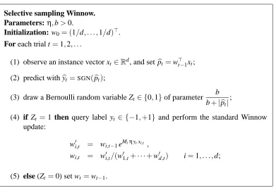
Selective sampling Winnow. Parameters: η,b>0.
Initialization: w0= (1/d, . . . ,1/d)⊤. For each trial t=1,2, . . .
(1) observe an instance vector xt ∈Rd, and set bpt=w⊤t−1xt; (2) predict withbyt =SGN(pbt);
(3) draw a Bernoulli random variable Zt ∈ {0,1}of parameter
b b+|bpt|
;
(4) if Zt =1 then query label yt ∈ {−1,+1} and perform the standard Winnow update:
w′i,t = wi,t−1eMtηytxi,t ,
wi,t = w′i,t/(w′1,t+···+w′d,t) i=1, . . . ,d; (5) else (Zt =0) set wt=wt−1.
Figure 4: A selective sampling version of the Winnow algorithm.
the update rule as follows:
w′i,t =wi,t−1eηytxi,t
wi,t =
w′i,t
∑d j=1w′j,t
for i=1, . . . ,d.
The theory behind the analysis of general additive family of algorithms shows that, notwithstand-ing their apparent diversity, Winnow and Perceptron are actually instances of the same additive algorithm.
To obtain a selective sampling version of Winnow we proceed exactly as we did in the previous cases: we query the label yt with probability b/(b+|pbt|), where|bpt|is the margin computed by the algorithm. The complete pseudo-code is described in Figure 4.
The mistake bound we prove for selective sampling Winnow is somewhat atypical since, unlike the Perceptron-like algorithms analyzed so far, the choice of the learning rateηgiven in this theorem is the same as the one suggested by the original Winnow analysis (see, e.g., Littlestone, 1989; Grove et al., 2001). Furthermore, since a meaningful bound in Winnow requiresηbe chosen in terms of
Theorem 4 If the algorithm of Figure 4 is run with parameters
η=2(1−α)γ
X2
∞ and b=αγ for someα∈(0,1)
on a sequence(x1,y1), . . . ,(xn,yn)∈Rd× {−1,+1}of examples such thatkxtk∞≤X∞for all t= 1, . . . ,n, then for all u∈Rd in the probability simplex,
E
" n
∑
t=1
Mt #
≤α1 Lγ,nγ(u)+ 1 2α(1−α)
X∞2ln d
γ2 .
As before, the expected number of labels queried by the algorithm equals∑tn=1Ehb+b|pbt|i.
Proof Similarly to the proof of Theorem 1, we estimate the influence of an update on the distance between the current weight wt−1and an arbitrary “target” hyperplane u, where in this case both vec-tors live in the probability simplex. Unlike the Perceptron analysis, based on the squared Euclidean distance, the analysis of Winnow uses the Kullback-Leibler divergence, or relative entropy,KL(·,·) to measure the progress of wt−1 towards u. The relative entropy of any two vectors u,v belonging to the probability simplex onRdis defined by
KL(u,v) = d
∑
i=1
uiln
ui
vi
.
Fix an arbitrary sequence(x1,y1), . . . ,(xn,yn)∈Rd× {−1,+1} of examples. As in the proof of Theorem 1, we have that MtZt=1 implies
η γ−ℓγ,t(u) = η γ−(γ−yt,u⊤xt)+
≤ ηytu⊤xt
= ηyt(u−wt−1+wt−1)⊤xt = ηyt(u−wt−1)⊤xt+ηytw⊤t−1xt .
Besides, exploiting a simple identity (as in the proof of Theorem 11.3 in Cesa-Bianchi and Lugosi, 2006, Chap. 5), we can rewrite the termηyt(u−wt−1)⊤xt as
ηyt(u−wt−1)⊤xt=KL(u,wt−1)−KL(u,wt) +ln d
∑
j=1
wj,t−1eηytvj !
where vj =xj−wt⊤−1xt. This equation is similar to the one obtained in the analysis of the selective sampling Perceptron algorithm, but for the relative entropy replacing the squared Euclidean dis-tance. Note, however, that the last term in the right-hand side of the above equation is not a relative entropy. To bound this last term, we consider the random variable X taking value xi,t ∈[−X∞,X∞] with probability wi,t−1. Then, from the Hoeffding inequality (Hoeffding, 1963) applied to X ,
ln d
∑
j=1
wj,t−1eηytvj !
=lnEheηyt(X−EX)
i
≤η
2 2 X
2
We plug back, rearrange and note that wt=wt−1whenever MtZt=0. This gets
MtZtη
γ+|pbt| −
η
2X 2
∞
≤MtZtηℓγ,t(u) +KL(u,wt−1)−KL(u,wt) , holding for any t. Summing over t=1, . . . ,n and dividing byηyields
n
∑
t=1
MtZt
γ+|pbt| −
η
2X 2
∞
≤ n
∑
t=1
MtZtℓγ,t(u) +
KL(u,w0)
η −
KL(u,wn)
η .
We drop the last term (which is nonpositive), and use KL(u,w0)≤ln d holding for any u in the probability simplex whenever w0= (1/d, . . . ,1/d). Then the above reduces to
n
∑
t=1
MtZt
γ+|bpt| −
η
2X 2
∞
≤ n
∑
t=1
MtZtℓγ,t(u) + ln d
η .
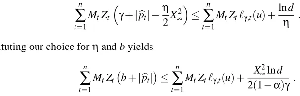
Substituting our choice forηand b yields n
∑
t=1
MtZt b+|pbt|
≤ n
∑
t=1
MtZtℓγ,t(u) +
X∞2ln d 2(1−α)γ.
To conclude, it suffices to exploitEt−1Zt =b/(b+|pbt|)and proceed as in the proof of the previous theorems.
4. Experiments
To investigate the empirical behavior of our algorithms we carried out a series of experiments on the first (in chronological order) 40,000 newswire stories from the Reuters Corpus Volume 1 (Reuters, 2000). Each story in this dataset is labelled with one or more elements from a set of 101 categories. In our experiments, we associated a binary classification task with each one of the 50 most frequent categories in the dataset, ignoring the remaining 51 (this was done mainly to reduce the effect of unbalanced datasets). All results presented in this section refer to the average performance over these 50 binary classification tasks. Though all of our algorithms are randomized, we did not com-pute averages over multiple runs of the same experiment, since we empirically observed that the variances of our statistics are quite small for the sample size taken into consideration.
To evaluate the algorithms we used the F-measure (harmonic average between precision and recall) since this is the most widespread performance index in text categorization experiments. Re-placing F-measure with classification accuracy yields results that are qualitatively similar to the ones shown here.
We focused on the following three algorithms: the selective sampling Perceptron algorithm of Figure 1 (here abbreviated asSEL-P), its adaptive version of Figure 2 (abbreviated asSEL-ADA), and the selective sampling second-order Perceptron algorithm of Figure 3 (abbreviated asSEL-2ND).
0.5 0.55 0.6 0.65 0.7 0.75
0.718 0.688 0.649 0.600 0.533 0.438 0.292
F-measure
Sampling rate
SEL-P SEL-P-FIXED SEL-P 100% rate
0.5 0.55 0.6 0.65 0.7 0.75
0.718 0.688 0.649 0.600 0.533 0.438 0.292
F-measure
Sampling rate
SEL-2ND SEL-2ND-FIXED SEL-2ND 100% rate
Figure 5: Comparison between margin-based sampling and random sampling with pre-specified sampling rate for the Perceptron algorithm (left) and the second-order Perceptron algo-rithm (right). The dotted lines show the performance obtained by querying all labels.
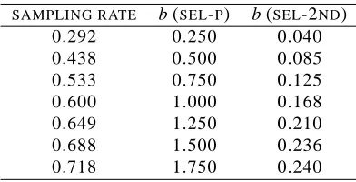
performance to the performance obtained by sampling each label with constant probability, i.e., the case when the Bernoulli random variables Zt in step (3) of Figure 1 have constant parameter equal to the desired sampling rate. We call this variantSEL-P-FIXED. The same experiment was repeated usingSEL-2NDand its fixed probability variantSEL-2ND-FIXED.
The following table shows the values of parameter b leading to the fixed sampling rates for both experiments.
SAMPLING RATE b (SEL-P) b (SEL-2ND)
0.292 0.250 0.040
0.438 0.500 0.085
0.533 0.750 0.125
0.600 1.000 0.168
0.649 1.250 0.210
0.688 1.500 0.236
0.718 1.750 0.240
0.2 0.3 0.4 0.5 0.6 0.7 0.8 0.9
0.4 0.6 0.8 1 1.2 1.4 1.6 1.8 2
F-measure and Sampling rate
Parameter b
F-measure Sampling rate
0.2 0.3 0.4 0.5 0.6 0.7 0.8 0.9
0.04 0.06 0.08 0.1 0.12 0.14 0.16 0.18 0.2
F-measure and Sampling rate
Parameter b
F-measure Sampling rate
Figure 6: Dependence of performance and sampling rate on the b parameter for the Perceptron algorithm (left) and the second-order Perceptron algorithm (right).
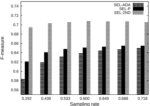
0.56 0.58 0.6 0.62 0.64 0.66 0.68 0.7 0.72 0.74
0.718 0.688 0.649 0.600 0.533 0.438 0.292
F-measure
Sampling rate
SEL-ADA SEL-P SEL-2ND
Figure 7: Performance level ofSEL-P,SEL-2ND, andSEL-ADAat different sampling rates.
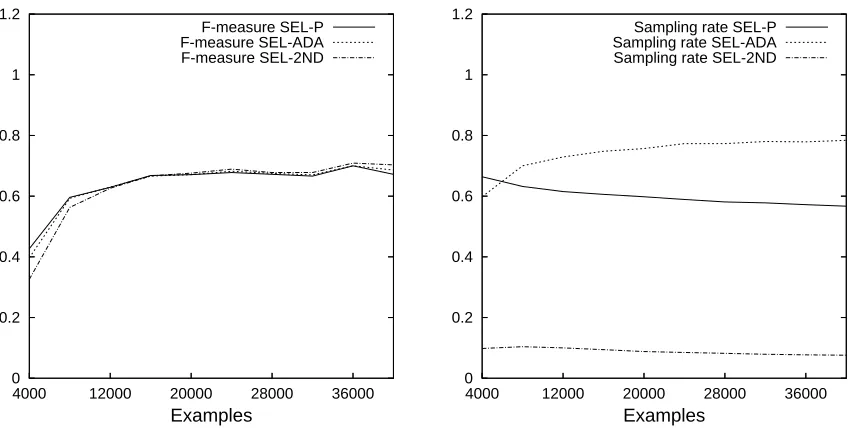
0 0.2 0.4 0.6 0.8 1 1.2
36000 28000
20000 12000
4000
Examples
F-measure SEL-P F-measure SEL-ADA F-measure SEL-2ND
0 0.2 0.4 0.6 0.8 1 1.2
36000 28000
20000 12000
4000
Examples
Sampling rate SEL-P Sampling rate SEL-ADA Sampling rate SEL-2ND
Figure 8: The right plot shows the sampling rates required by different algorithms to achieve a given target performance value (shown in the left plot).
(and SEL-ADA) might be an indication that the second-order Perceptron tends to achieve a larger margin than the standard Perceptron, but we do not have a clear explanation for this phenomenon.
5. Conclusions and Open Problems
We have introduced a general technique for turning linear-threshold algorithms from the general additive family into selective sampling algorithms. We have analyzed these algorithms in a worst-case on-line learning setting, providing bounds on the expected number of mistakes. Our theoretical investigation naturally arises from the traditional way margin-based algorithms are analyzed in the mistake bound model of on-line learning (Littlestone, 1988; Grove et al., 2001; Gentile and War-muth, 1999; Freund and Schapire, 1999; Gentile, 2003; Cesa-Bianchi et al., 2005). This investi-gation suggests that our semi-supervised algorithms can achieve, on average, the same accuracy as that of their fully supervised counterparts, but allowing a substantial saving of labels. When applied to (kernel-based) Perceptron-like algorithms, label saving directly implies higher sparsity for the computed classifier which, in turn, yields a running time saving in both training and test phases.
Our theoretical results are corroborated by an empirical comparison on textual data. In these experiments we have shown that proper choices of the scaling parameter b yield a significant re-duction in the rate of queried labels without causing an excessive degradation of the classification performance. In addition, we have also shown that by fixing ahead of time the total number of label observations, the margin-driven way of distributing these observations over the training set is largely more effective than a random one.
no prior information, a bound on the expected number of mistakes having the same form as the one achieved by choosing the “best” b in hindsight. Now, it is intuitively clear that the number of prediction mistakes and the number of queried labels can be somehow traded-off against each other. Within this trade-off, the above “best” choice is only aimed at minimizing mistakes, rather than queried labels. In fact, the practical utility of this adaptive algorithm seems, at present, fairly limited.
There are many ways this work could be extended. Perhaps the most important is being able to quantify the expected number of requested labels as a function of the problem parameters (margin of the data and so on). It is worth observing that for the adaptive version of the selective sampling Perceptron (Figure 2) we can easily derive a lower bound on the label sampling rate. Assume for simplicity thatkxtk=1 for all t. Then we can write
bt−1
bt−1+|bpt|
= β
√
1+Kt−1
β√1+Kt−1+|w⊤t−1xt|
≥ β
√
1+Kt−1
β√1+Kt−1+kwt−1k
≥ β
√
1+Kt−1
β√1+Kt−1+√Kt−1
(using Inequality (7))
≥ β+β1
holding for any trial t. Is it possible to obtain a meaningful upper bound? At first glance, this requires a lower bound on the margin|pbt|. But since there are no guarantees on the margin the algorithm achieves (even in the separable case), this route does not look profitable. Would such an argument work for on-line large margin algorithms, such as those by Li and Long (2002) and Gentile (2001)?
As a related issue, our theorems do not make any explicit statement about the number of weight updates (i.e., support vectors) computed by our selective sampling algorithms. We would like to see a theoretical argument that enables us to combine the bound on the number of mistakes with a bound on the number of labels, resulting in an informative upper bound on the number of updates.
Finally, the adaptive parameter version of Figure 2 centers on inequalities such as (7) to deter-mine the current label request rate. It seems these inequalities are too coarse to make the algorithm effective in practice. Our experiments basically show that this algorithm tends to query more labels than needed. It turns out there are many ways one can modify this algorithm to make it less “cau-tious”, though this gives rise to algorithms which seem to escape a crisp mathematical analysis. We would like to devise an adaptive parameter version of the selective sampling Perceptron algorithm that both lends itself to formal analysis and is competitive in practice.
Acknowledgments
The authors gratefully acknowledge partial support by the PASCAL Network of Excellence under EC grant no. 506778. This publication only reflects the authors’ views.
References
D. Angluin. Queries and concept learning. Machine Learning, 2(4):319–342, 1988.
P. Auer, N. Cesa-Bianchi, and C. Gentile. Adaptive and self-confident on-line learning algorithms.
Journal of Computer and System Sciences, 64:48–75, 2002.
K. S. Azoury and M. K. Warmuth. Relative loss bounds for on-line density estimation with the exponential familiy of distributions. Machine Learning, 43(3):211–246, 2001.
H. D. Block. The Perceptron: A model for brain functioning. Reviews of Modern Physics, 34: 123–135, 1962.
A. Bordes, S. Ertekin, J. Weston, and L. Bottou. Fast kernel classifiers with online and active learning. Journal of Machine Learning reserarch, 6:1579–1619, 2005.
C. Campbell, N. Cristianini, and A. Smola. Query learning with large margin classifiers. In
Pro-ceedings of the 17th International Conference on Machine Learning, pages 111–11. Morgan
Kaufman, 2000.
N. Cesa-Bianchi, A. Conconi, and C. Gentile. Learning probabilistic linear-threshold classifiers via selective sampling. In Proceedings of the 16th Annual Conference on Learning Theory, LNAI
2777, pages 373–386. Springer, 2003.
N. Cesa-Bianchi, A. Conconi, and C. Gentile. A second-order Perceptron algorithm. SIAM Journal
on Computing, 43(3):640–668, 2005.
N. Cesa-Bianchi and G. Lugosi. Potential-based algorithms in on-line prediction and game theory.
Machine Learning, 51(3):239–261, 2003.
N. Cesa-Bianchi and G. Lugosi. Prediction, Learning, and Games. Cambridge University Press, 2006.
R. Cohn, L. Atlas, and R. Ladner. Training connectionist networks with queries and selective sampling. In Advances in Neural Information Processing Systems 2. MIT Press, 1990.
N. Cristianini and J. Shawe-Taylor. An Introduction to Support Vector Machines. Cambridge Uni-versity Press, 2001.
S. Dasgupta, A. T. Kalai, and C. Monteleoni. Analysis of Perceptron-based active learning. In
Proceedings of the 18th Annual Conference on Learning Theory, LNAI 2777, pages 249–263.
Springer, 2005.
R. Duda and P. Hart, and D. Stork. Pattern classification, second edition. Wiley Interscience, 2000. J. Forster. On relative loss bounds in generalized linear regression. In Proceedings of the 12th
International Symposium on Fundamentals of Computation Theory, LNCS 1684, pages 269–280.
Springer, 1999.
Y. Freund and R. Schapire. Large margin classification using the Perceptron algorithm. Machine
Learning, 37(3):277–296, 1999.
Y. Freund, S. Seung, E. Shamir, and N. Tishby. Selective sampling using the query by committee algorithm. Machine Learning, 28(2/3):133–168, 1997.
C. Gentile. A new approximate maximal margin classification algorithm. Journal of Machine
Learning Research, 2:213–242, 2001.
C. Gentile. The robustness of the p-norm algorithms. Machine Learning, 53(3):265–299, 2003. C. Gentile and M. Warmuth. Linear hinge loss and average margin. In Advances in Neural
Infor-mation Processing Systems 10, pages 225–231. MIT Press, 1999.
A. J. Grove, N. Littlestone, and D. Schuurmans. General convergence results for linear discriminant updates. Machine Learning, 43(3):173–210, 2001.
D. P. Helmbold, N. Littlestone, and P. M. Long. Apple tasting. Information and Computation, 161 (2):85–139, 2000.
D. P. Helmbold and S. Panizza. Some label efficient learning results. In Proceedings of the 10th
Annual Conference on Computational Learning Theory, pages 218–230. ACM Press, 1997.
M. Herbster and M. K. Warmuth. Tracking the Best Linear Predictor. Journal of Machine Learning
Research, 1: 281–309, 2001.
W. Hoeffding. Probability inequalities for sums of bounded random variables. Journal of the
American Statistical Association, 58:13–30, 1963.
J. Kivinen and M. K. Warmuth. Relative loss bounds for multidimensional regression problems.
Machine Learning, 45(3):301–329, 2001.
T. L. Lai and C. Z. Wei. Least squares estimates in stochastic regression models with applications to identification and control of dynamic systems. The Annals of Statistics, 10(1):154–166, 1982. Y. Li and P. Long. The relaxed online maximum margin algorithm. Machine Learning, 46:361–387,
2002.
N. Littlestone. Learning quickly when irrelevant attributes abound: a new linear-threshold algo-rithm. Machine Learning, 2(4):285–318, 1988.
N. Littlestone. Mistake Bounds and Logarithmic Linear-threshold Learning Algorithms. PhD thesis, University of California Santa Cruz, 1989.
A. B. J. Novikov. On convergence proofs on Perceptrons. In Proceedings of the Symposium on the
Reuters. Reuters corpus vol. 1, 2000.
URLabout.reuters.com/researchandstandards/corpus/.
F. Rosenblatt. The Perceptron: A probabilistic model for information storage and organization in the brain. Psychological Review, 65:386–408, 1958.
B. Sch¨olkopf and A. Smola. Learning with Kernels. MIT Press, 2002.
S. Tong and D. Koller. Support vector machine active learning with applications to text classifica-tion. In Proceedings of the 17th International Conference on Machine Learning, pages 999–1006. Morgan Kaufmann, 2000.
V. N. Vapnik. Statistical Learning Theory. Wiley, 1998.
M. K. Warmuth and A. K. Jagota. Continuous and discrete-time nonlinear gradient descent: Relative loss bounds and convergence. In Electronic proceedings of the 5th International Symposium on