Algorithms and Hardness Results for Parallel Large Margin Learning
Philip M. Long [email protected]
Microsoft
1020 Enterprise Way Sunnyvale, CA 94089
Rocco A. Servedio [email protected]
Department of Computer Science Columbia University
1214 Amsterdam Ave., Mail Code: 0401 New York, NY 10027
Editor:Yoav Freund
Abstract
We consider the problem of learning an unknown large-margin halfspace in the context of parallel computation, giving both positive and negative results.
As our main positive result, we give a parallel algorithm for learning a large-margin half-space, based on an algorithm of Nesterov’s that performs gradient descent with a momentum term. We show that this algorithm can learn an unknownγ-margin halfspace overn dimensions using
n·poly(1/γ)processors and running in time ˜O(1/γ) +O(logn). In contrast, naive parallel algo-rithms that learn aγ-margin halfspace in time that depends polylogarithmically onnhave an inverse quadratic running time dependence on the margin parameterγ.
Our negative result deals with boosting, which is a standard approach to learning large-margin halfspaces. We prove that in the original PAC framework, in which a weak learning algorithm is provided as an oracle that is called by the booster, boosting cannot be parallelized. More precisely, we show that, if the algorithm is allowed to call the weak learner multiple times in parallel within a single boosting stage, this ability does not reduce the overall number of successive stages of boosting needed for learning by even a single stage. Our proof is information-theoretic and does not rely on unproven assumptions.
Keywords: PAC learning, parallel learning algorithms, halfspace learning, linear classifiers
1. Introduction
One of the most fundamental problems in machine learning is learning an unknown halfspace from labeled examples that satisfy amargin constraint,meaning that no example may lie too close to the separating hyperplane. In this paper we consider large-margin halfspace learning in the PAC (prob-ably approximately correct) setting of learning from random examples: there is a target halfspace
f(x) =sign(w·x), wherewis an unknown unit vector, and an unknown probability distribution
D
over the unit ballBn={x∈Rn:kxk2≤1}which is guaranteed to have support contained in the set{x∈Bn:|w·x| ≥γ}of points that have Euclidean margin at leastγrelative to the separating
where eachxis independently drawn from
D
, and it must with high probability output a (1−ε) -accurate hypothesis, that is, a hypothesish:Rn→ {−1,1}that satisfies Prx∼D[h(x)6=f(x)]≤ε.One of the earliest, and still most important, algorithms in machine learning is the perceptron algorithm (Block, 1962; Novikoff, 1962; Rosenblatt, 1958) for learning a large-margin halfspace. The perceptron is an online algorithm but it can be easily transformed to the PAC setting described above (Vapnik and Chervonenkis, 1974; Littlestone, 1989; Freund and Schapire, 1999); the resulting PAC algorithms run in poly(n,1
γ,1ε)time, useO(εγ12)labeled examples inRn, and learn an unknown
n-dimensionalγ-margin halfspace to accuracy 1−ε.
A motivating question: achieving perceptron’s performance in parallel? The last few years have witnessed a resurgence of interest in highly efficient parallel algorithms for a wide range of computational problems in many areas including machine learning (Workshop, 2009, 2011). So a natural goal is to develop an efficient parallel algorithm for learning γ-margin halfspaces that matches the performance of the perceptron algorithm. A well-established theoretical notion of efficient parallel computation (see, for example, the text by Greenlaw et al. (1995) and the many references therein) is that an efficient parallel algorithm for a problem with input sizeNis one that uses poly(N) processors and runs in parallel time polylog(N). Since the input to the perceptron algorithm is a sample of poly(1ε,1γ)labeled examples inRn, we naturally arrive at the following:
Main Question: Is there a learning algorithm that uses poly(n,1γ,1ε) processors and runs in time poly(logn,log1γ,log1ε)to learn an unknownn-dimensionalγ-margin half-space to accuracy 1−ε?
Following Vitter and Lin (1992), we use a CRCW PRAM model of parallel computation. This abstracts away issues like communication and synchronization, allowing us to focus on the most fundamental issues. Also, as did Vitter and Lin (1992), we require that an efficient parallel learning algorithm’s hypothesis must be efficiently evaluatable in parallel, since otherwise all the computa-tion required to run any polynomial-time learning algorithm could be “offloaded” onto evaluating the hypothesis. Because halfspace learning algorithms may be sensitive to issues of numerical pre-cision, these are not abstracted away in our model; we assume that numbers are represented as rationals.
As noted by Freund (1995) (see also Lemma 2 below), the existence of efficient boosting algorithms such as the algorithms of Freund (1995) and Schapire (1990) implies that any PAC learning algorithm can be efficiently parallelized in terms of its dependence on the accuracy pa-rameter ε: more precisely, any PAC learnable class C of functions can be PAC learned to ac-curacy 1−ε using O(1/ε) processors by an algorithm whose running time dependence on ε is
O(log 1ε·poly(log log(1/ε))),by boosting an algorithm that learns to accuracy (say) 9/10. We may thus equivalently restate the above question as follows.
Main Question (simplified):Is there a learning algorithm that uses poly(n,1γ) proces-sors and runs in time poly(logn,log1γ) to learn an unknown n-dimensional γ-margin halfspace to accuracy 9/10?
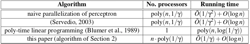
Algorithm No. processors Running time
naive parallelization of perceptron poly(n,1/γ) O˜(1/γ2) +O(logn) (Servedio, 2003) poly(n,1/γ) O˜(1/γ2) +O(logn) poly-time linear programming (Blumer et al., 1989) 1 poly(n,log(1/γ))
this paper (algorithm of Section 2) n·poly(1/γ) O˜(1/γ) +O(logn)
Table 1: Bounds on various parallel algorithms for learning aγ-margin halfspace overRn.
1.1 Relevant Prior Results
Table 1 summarizes the running time and number of processors used by various parallel algorithms to learn aγ-margin halfspace overRn.
The naive parallelization of perceptron in the first line of the table is an algorithm that runs for
O(1/γ2)stages. In each stage it processes all of theO(1/γ2)examples simultaneously in parallel, identifies one that causes the perceptron algorithm to update its hypothesis vector, and performs this update. Since the examples aren-dimensional this can be accomplished inO(log(n/γ))time using
O(n/γ2)processors; the mistake bound of the online perceptron algorithm is 1/γ2, so this gives a running time bound of ˜O(1/γ2)·logn.We do not see how to obtain parallel time bounds better than
O(1/γ2)from recent analyses of other algorithms based on gradient descent (Collins et al., 2002; Dekel et al., 2011; Bradley et al., 2011), some of which use assumptions incomparable in strength to theγ-margin condition studied here.
The second line of the table corresponds to a similar naive parallelization of the boosting-based algorithm of Servedio (2003) that achieves perceptron-like performance for learning a γ-margin halfspace. This algorithm boosts forO(1/γ2) stages over a O(1/γ2)-size sample. At each stage of boosting this algorithm computes a real-valued weak hypothesis based on the vector average of the (normalized) examples weighted according to the current distribution; since the sample size is
O(1/γ2) this can be done inO(log(n/γ))time using poly(n,1/γ)processors. Since the boosting algorithm runs forO(1/γ2)stages, the overall running time bound is ˜O(1/γ2)·logn.(For both this algorithm and the perceptron the time bound can be improved to ˜O(1/γ2) +O(logn)as claimed in the table by using an initial random projection step. We show how to do this in Section 2.3.)
The third line of the table, included for comparison, is simply a standard sequential algorithm for learning a halfspace based on polynomial-time linear programming executed on one processor (Blumer et al., 1989; Karmarkar, 1984).
In addition to the results summarized in the table, we note that efficient parallel algorithms have been developed for some simpler PAC learning problems such as learning conjunctions, disjunc-tions, and symmetric Boolean functions (Vitter and Lin, 1992). Bshouty et al. (1998) gave efficient parallel PAC learning algorithms for some geometric constant-dimensional concept classes. Collins et al. (2002) presented a family of boosting-type algorithms that optimize Bregman divergences by updating a collection of parameters in parallel; however, their analysis does not seem to imply that the algorithms need fewer thanΩ(1/γ2)stages to learnγ-margin halfspaces.
main question for several reasons: first, the main question allows any hypothesis representation that can be efficiently evaluated in parallel, whereas the hardness result requires the hypothesis to be a halfspace. Second, the main question allows the algorithm to use poly(n,1/γ)processors and to run in poly(logn,log1γ) time, whereas the hardness result of Vitter and Lin (1992) only rules out algorithms that use poly(n,log1γ)processors and run in poly(logn,log log1γ)time. Finally, the main question allows the final hypothesis to err on up to (say) 5% of the points in the data set, whereas the hardness result of Vitter and Lin (1992) applies only to algorithms whose hypotheses correctly classify all points in the data set.
Finally, we note that the main question has an affirmative answer if it is restricted so that either the number of dimensionsn or the margin parameterγis fixed to be a constant (so the resulting restricted question asks whether there is an algorithm that uses polynomially many processors and polylogarithmic time in the remaining parameter). Ifγis fixed to a constant then either of the first two entries in Table 1 gives a poly(n)-processor,O(logn)-time algorithm. Ifnis fixed to a constant then the efficient parallel algorithm of Alon and Megiddo (1994) for linear programming in constant dimension can be used to learn aγ-margin halfspace using poly(1/γ)processors in polylog(1/γ)
running time (see also Vitter and Lin, 1992, Theorem 3.4).
1.2 Our Results
We give positive and negative results on learning halfspaces in parallel that are inspired by the main question stated above.
1.2.1 POSITIVERESULTS
Our main positive result is a parallel algorithm for learning large-margin halfspaces, based on a rapidly converging gradient method due to Nesterov (2004), which usesO(n·poly(1/γ))processors to learnγ-margin halfspaces in parallel time ˜O(1/γ) +O(logn)(see Table 1). (An earlier version of this paper (Long and Servedio, 2011) analyzed on algorithm based on interior-point methods from convex optimization and fast parallel algorithms for linear algebra, showing that it uses poly(n,1/γ)
processors to learnγ-margin halfspaces in parallel time ˜O(1/γ) +O(logn).) We are not aware of prior parallel algorithms that provably learnγ-margin halfspaces running in time polylogarithmic in
nand subquadratic in 1/γ.
We note that simultaneously and independently of the initial conference publication of our work (Long and Servedio, 2011), Soheili and Pe˜na (2012) proposed a variant of the perceptron algorithm and shown that it terminates inO
√
logn γ
iterations rather than the 1/γ2iterations of the original perceptron algorithm. Like our algorithm, the Soheili and Pe˜na (2012) algorithm uses ideas of Nes-terov (2005). Soheili and Pe˜na (2012) do not discuss a parallel implementation of their algorithm, but since their algorithm performs ann-dimensional matrix-vector multiplication at each iteration, it appears that a parallel implementation of their algorithm would useΩ(n2)processors and would have parallel running time at least Ω(logγn)3/2(assuming that multiplying a n×n matrix by an
n×1 vector takes parallel timeΘ(logn)usingn2processors). In contrast, our algorithm requires a linear number of processors as a function ofn, and has parallel running time ˜O(1/γ) +O(logn).1
1.2.2 NEGATIVERESULTS
By modifying our analysis of the algorithm we present, we believe that it may be possible to estab-lish similar positive results for other formulations of the large-margin learning problem, including ones (see Shalev-Shwartz and Singer, 2010) that have been tied closely to weak learnability. In contrast, our main negative result is an information-theoretic argument that suggests that such pos-itive parallel learning results cannot be obtained by boosting alone. We show that in a framework where the weak learning algorithm must be invoked as an oracle, boosting cannot be parallelized: being able to call the weak learner multiple times in parallel within a single boosting stage does not reduce the overall number of sequential stages of boosting that are required. We prove that any par-allel booster must performΩ(log(1/ε)/γ2)sequential stages of boosting a “black-box”γ-advantage weak learner to learn to accuracy 1−ε in the worst case; this extends an earlierΩ(log(1/ε)/γ2) lower bound of Freund (1995) for standard (sequential) boosters that can only call the weak learner once per stage.
2. An Algorithm Based on Nesterov’s Algorithm
In this section we describe and analyze a parallel algorithm for learning aγ-margin halfspace. The algorithm of this section applies an algorithm of Nesterov (2004) that, roughly speaking, approxi-mately minimizes a suitably smooth convex function to accuracyεusingO(p
1/ε)iterative steps (Nesterov, 2004), each of which can be easily parallelized.
Directly applying the basic Nesterov algorithm gives us an algorithm that usesO(n)processors, runs in parallel timeO(log(n)·(1/γ)), and outputs a halfspace hypothesis that has constant accu-racy. By combining the basic algorithm with random projection and boosting we get the following stronger result:
Theorem 1 There is a parallel algorithm with the following performance guarantee: Let f,
D
de-fine an unknownγ-margin halfspace overBn. The algorithm is given as inputε,δ>0and access to labeled examples(x,f(x))that are drawn independently fromD
.It runs inO(((1/γ)polylog(1/γ) +log(n))log(1/ε)poly(log log(1/ε)) +log log(1/δ))
parallel time, uses
n·poly(1/γ,1/ε,log(1/δ))
processors, and with probability1−δit outputs a hypothesis h satisfyingPrx∼D[h(x)6= f(x)]≤ε.
We assume that the value ofγis “known” to the algorithm, since otherwise the algorithm can use a standard “guess and check” approach trying γ=1,1/2,1/4,etc., until it finds a value that works.
Freund (1995) indicated how to parallelize his boosting-by-filtering algorithm. In Appendix A, we provide a detailed proof of the following lemma.
Lemma 2 (Freund, 1995) Let
D
be a distribution over (unlabeled) examples. Let A be a par-allel learning algorithm, and cδ and cε be absolute positive constants, such that for allD
′ with-4 -2 2 4 2
4 6 8 10
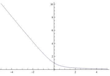
Figure 1: A plot of a loss functionφused in Section 2.
support(
D
′)⊆support(D
), given draws(x,f(x))fromD
′, with probability cδ, A outputs a hypothe-sis with accuracy12+cε(w.r.t.D
′) usingP
processors inT
time. Then there is a parallel algorithm B that, given access to independent labeled examples (x,f(x))drawn fromD
, with probability1−δ, constructs a (1−ε)-accurate hypothesis (w.r.t.
D
) in O(T
log(1/ε)poly(log log(1/ε)) +log log(1/δ))time usingpoly(
P
,1/ε,log(1/δ))processors.In Section 2.1 we describe the basic way that Nesterov’s algorithm can be used to find a half-space hypothesis that approximately minimizes a smooth loss function over a set ofγ-margin labeled examples. (This section has nothing to do with parallelism.) Then later we explain how this algo-rithm is used in the larger context of a parallel algoalgo-rithm for halfspaces.
2.1 The Basic Algorithm
LetS= (x1,y1), . . . ,(xm,ym)be a data set ofmexamples labeled according to the targetγ-margin
halfspace f; that is,yi=f(xi)for alli.
We will apply Nesterov’s algorithm to minimize a regularized loss as follows.
The loss part.Forz∈Rwe define
φ(z) =p1+z2−z. (See Figure 1 for a plot ofφ.) Forv∈Rnwe define
Φ(v) = 1
m m
∑
t=1φ(yt(v·xt)).
The regularization part. We define a regularizer
R(v) =γ2kvk2/100 wherek · kdenotes the 2-norm.
We will apply Nesterov’s iterative algorithm to minimize the following function
Ψ(v) =Φ(v) +R(v).
AlgorithmANes:
• Setµ=γ2/50,L=51/50.
• Initializev0=z0=0.
• For eachk=0,1, . . ., set
– vk+1=zk−L1g(zk), and
– zk+1=vk+1+
√ L−√µ √
L+√µ(vk+1−vk).
We begin by establishing various bounds onΨthat Nesterov uses in his analysis ofANes. Lemma 3 The gradient g ofΨhas a Lipschitz constant at most51/50.
Proof:We have
∂Ψ ∂vi =
1
m
∑
t φ ′(yt(v·xt))ytxt,i+γ2vi/50
and hence, writingg(v)to denote the gradient ofΨatv, we have
g(v) = 1
m
∑
t φ ′(yt(v·xt))ytxt+γ2v/50.
Chooser∈Rn. Applying the triangle inequality, we have
||g(v)−g(r)|| =
1
m
∑
t (φ′(yt(v·x
t))−φ′(yt(r·xt)))ytxt+γ2(v−r)/50
≤ 1
m
∑
t ||(φ ′(yt(v·xt))−φ′(yt(r·xt)))ytxt||+γ2||v−r||/50 ≤ m1
∑
t
|φ′(yt(v·xt))−φ′(yt(r·xt))|+γ2||v−r||/50,
since each vectorxt has length at most 1. Basic calculus gives thatφ′′is always at most 1, and hence
|φ′(yt(v·xt))−φ′(yt(r·xt))| ≤ |v·xt−r·xt| ≤ ||v−r||,
again sincext has length at most 1. The bound then follows from the fact thatγ2≤1.
We recall the definition of strong convexity (Nesterov, 2004, pp. 63–64): a multivariate function
qisµ-strongly convex if for allv,wand allα∈[0,1]it holds that
q(αv+ (1−α)w)≤αq(v) + (1−α)q(w)−µα(1−α)||v−w|| 2
2 .
(For intuition’s sake, it may be helpful to note that a suitably smoothqisµ-strongly convex if any restriction of q to a line has second derivative that is always at least µ.) We recall the fact that strongly convex functions have unique minimizers.
Proof: This follows directly from the fact that µ=γ2/50, Φ is convex, and ||v||2 is 2-strongly convex.
Given the above, the following lemma is an immediate consequence of Theorem 2.2.3 of Nes-terov’s (2004) book. The lemma upper bounds the difference betweenΨ(vk), wherevk is the point
computed in thek-th iteration of Nesterov’s algorithmANes, and the true minimum value ofΨ. A proof is in Appendix B.
Lemma 5 Letwbe the minimizer ofΨ. For each k, we haveΨ(vk)−Ψ(w)≤4L(1+µ||w||
2/2)
(2√L+k√µ)2 .
2.2 The Finite Precision Algorithm
The algorithm analyzed in the previous subsection computes real numbers with infinite precision. Now we will analyze a finite precision variant of the algorithm, which we callANfp(for “Nesterov finite precision”).
(We note that d’Aspremont 2008, also analyzed a similar algorithm with an approximate gra-dient, but we were not able to apply his results in our setting because of differences between his assumptions and our needs. For example, the algorithm described by d’Aspremont 2008, assumed that optimization was performed over a compact setC, and periodically projected solutions ontoC; it was not obvious to us how to parallelize this algorithm.)
We begin by writing the algorithm as if it took two parameters, γand a precision parameter
β>0. The analysis will show how to setβas a function ofγ. To distinguish betweenANfpandANes we use hats throughout our notation below.
AlgorithmANfp:
• Setµ=γ2/50,L=51/50.
• Initialize ˆv0=zˆ0=0.
• For eachk=0,1, . . .,
– Let ˆrk be such that||rˆk−1Lg(ˆzk)|| ≤β. Set
– vˆk+1=zˆk−ˆrk, and
– zˆk+1=vˆk+1+
√ L−√µ √
L+√µ(vˆk+1−vˆk).
We discuss the details of exactly how this finite-precision algorithm is implemented, and the parallel running time required for such an implementation, at the end of this section.
Our analysis of this algorithm will proceed by quantifying how closely its behavior tracks that of the infinite-precision algorithm.
Lemma 6 Let v0,v1, ... be the sequence of points computed by the infinite precision version of
Nesterov’s algorithm, andvˆ0,vˆ1, ...be the corresponding finite-precision sequence. Then for all k,
we have||vk−vˆk|| ≤β·7k.
Proof: Let ˆsk=rˆk−g(zˆk).Our proof is by induction, with the additional inductive hypothesis that ||zk−zˆk|| ≤3β·7k.
We have
||vk+1−vˆk+1||=
(zk−
1
Lg(zk))−(zˆk−(
1
Lg(zˆk) +ˆsk) ,
and, using the triangle inequality, we get
||vk+1−vˆk+1|| ≤ ||zk−zˆk||+ 1
Lg(zk)−(
1
Lg(zˆk) +ˆsk)
≤ 3β·7k+ 1
Lg(zk)−(
1
Lg(zˆk) +ˆsk)
≤ 3β·7k+1
L||g(zk)−g(zˆk)||+||sˆk|| (triangle inequality) ≤ 3β·7k+||zk−zˆk||+||ˆsk|| (by Lemma 3)
≤ 3β·7k+3β·7k+β (by definition of ˆsk)
< β·7k+1.
Also, we have
||zk+1−zˆk+1|| =
2 1+p
µ/L(vk+1−vˆk+1)− √
L−√µ √
L+√µ(vk−vˆk) ≤ 2 1+p
µ/L(vk+1−vˆk+1) + √ L−√µ √
L+√µ(vk−vˆk) ≤ 2||vk+1−vˆk+1||+||vk−vˆk||
≤ 2β·7k+1+β·7k
≤ 3β·7k+1,
completing the proof.
2.3 Application to Learning
Now we are ready to prove Theorem 1. By Lemma 2 it suffices to prove the theorem in the case in whichε=7/16 andδ=1/2.
We may also potentially reduce the number of variables by applying a random projection. We say that arandom projection matrixis a matrixAchosen uniformly from{−1,1}n×d. Given such an Aand a unit vector w∈Rn (defining a target halfspace f(x) =sign(w·x)), let w′ denote the
vector(1/√d)wA∈Rd. After transformation byAthe distribution
D
overBn is transformed to adistribution
D
′overRdin the natural way: a drawx′fromD
′is obtained by making a drawxfromD
and settingx′= (1/√d)xA. We will use the following lemma, which is a slight variant of known lemmas (Arriaga and Vempala, 2006; Blum, 2006); we prove this exact statement in Appendix C.Lemma 7 Let f(x) =sign(w·x)and
D
define aγ-margin halfspace as described in the introduc-tion. For d=O((1/γ2)log(1/γ)),a random n×d projection matrix A will with probability99/100induce
D
′andw′ as described above such thatPrx′∼D′ h
w′
kw′k·x′
<γ/2 or kx
The algorithm first selects ann×drandom projection matrixAwhered=O(log(1/γ)/γ2). This defines a transformationΦA:Bn→Rdas follows: givenx∈Bn,the vectorΦA(x)∈Rd is obtained
by
(i) rounding eachxi to the nearest integer multiple of 1/(4⌈ p
n/γ⌉); then
(ii) settingx′= 1 2√d
xA(we scale down by an additional factor of two to get examples that are contained in the unit ballBd); and finally
(iii) rounding eachx′i to the nearest multiple of 1/(8⌈d/γ⌉).
Givenx it is easy to computeΦA(x)using O(nlog(1/γ)/γ2) processors inO(log(n/γ))time. Let
D
′ denote the distribution over Rd obtained by applying ΦA toD
. Across all coordinatesD
′ issupported on rational numbers with the same poly(1/γ)common denominator. By Lemma 7, with probability 99/100
Pr
x′∼D′ h
x′·(w′/kw′k) <γ′
def
=γ/8 or kx′k2>1
i ≤γ4.
Our algorithm drawsc0dexamples by sampling from
D
′. Applying Lemma 7, we may assume without loss of generality that our examples haved=O(log(1/γ)/γ2)and that the marginγ′ afterthe projection is at least Θ(γ), and that all the coordinates of all the examples have a common denominator which is at most poly(1/γ).Thus far the algorithm has usedO(log(n/γ))parallel time andO(nlog(1/γ)/γ2)many processors.
Next, the algorithm appliesANfpfrom the previous section forKstages, whereK=⌈c1/γ′⌉and
β=c27−K. Herec0, c1, and c2 are absolute positive constants; our analysis will show that there exist choices of these constants that give Theorem 1.
For our analysis, as before, let wbe the minimizer ofΨ, and letube a unit normal vector for the target halfspace f(x) =sign(u·x). (We emphasize thatΨis now defined using the projected
d-dimensional examples and withγ′in place ofγin the definition of the regularizerR.)
Our first lemma gives an upper bound on the optimal value of the objective function.
Lemma 8 Ψ(w)≤0.26.
Proof Sincewis the minimizer ofΨwe haveΨ(w)≤Ψ(3u/γ′).In turnΨ(3u/γ′)is easily seen to be at mostφ(3) +9/100≤0.26, since every example has margin at leastγ′with respect tou.
Next, we bound the norm ofw.
Lemma 9 ||w||2≤26/γ′2. Proof:The definition ofΨgives
||w||2≤100Ψ(w)/γ′2
and combining with Lemma 8 gives||w||2≤26/γ′2. Now we can bound the objective function value ofvK.
Proof:Plugging Lemma 9 into the RHS of Lemma 5 and simplifying, we get
Ψ(vK)−Ψ(w)≤
751
25(2√51+γ′K)2. Applying Lemma 8, we get
Ψ(vK)≤0.26+
751
25(2√51+γ′K)2. from which the lemma follows.
Now we can boundvK nearly the same way that we boundedw:
Lemma 11 ||vK|| ≤7/γ′.
Proof:The argument is similar to the proof of Lemma 9, using Lemma 10 in place of Lemma 8. Now we can bound the value of the objective function of the finite precision algorithm.
Lemma 12 There exist absolute positive constants c1,c2such thatΨ(vˆK)≤3/7.
Proof Becauseβ=c27−⌈c1/γ ′⌉
, Lemma 6 implies that ||vˆK−vK|| ≤c2. Sinceφhas a Lipschitz constant of 2, so doesΦ, and consequently we have that
Φ(vˆK)−Φ(vK)≤2c2. (1) Next, since Lemma 11 gives||vK|| ≤7/γ′, and||vˆK−vK|| ≤c2, we have||vˆK|| ≤7/γ′+c2, which in turn implies
kvˆKk2− kvKk2≤(7/γ′+c2)2−(7/γ′)2=14c2/γ′+c22. and thus
R(vˆK)−R(vK)≤
14c2γ′ 100 +
(γ′)2c2 2 100 .
Combining this with (1), we get that forc2less than a sufficiently small positive absolute constant, we haveΨ(vˆK)−Ψ(vK)<3/7−2/5, and combining with Lemma 10 completes the proof.
Finally, we observe thatΨ(vˆk)is an upper bound on the fraction of examples in the sample that
are misclassified by ˆvk. Takingc0 sufficiently large and applying standard VC sample complexity bounds, we have established the(ε,δ)PAC learning properties of the algorithm. (Recall from the start of this subsection that we have takenε=7/16 andδ=1/2.)
It remains to analyze the parallel time complexity of the algorithm. We have already analyzed the parallel time complexity of the initial random projection stage, and shown that we may take the finite-precision iterative algorithmANfpto run forO(1/γ)stages, so it suffices to analyze the parallel time complexity of each stageANfp.We will show that each stage runs in parallel time polylog(1/γ) and thus establish the theorem.
Recall that we have setβ=Θ(7−K)and thatK=Θ(1/γ).The invariant we maintain throughout each iterationkof algorithmANfpis that each coordinate of ˆvk is a poly(K)-bit rational number and
each coordinate of ˆzkis a poly(K)-bit rational number. It remains to show that given such values ˆvk
1. it is possible to compute each coordinateg(zˆk)ito accuracy 2−100K/ √
d;
2. it is possible to determine a vector ˆrksuch thatkrˆk−g(zˆk)k ≤β, and that each coefficient of
the new value ˆvk+1=zˆk−ˆrkis again a poly(K)-bit rational number; and
3. it is possible to compute the new value ˆzk+1 and that each coordinate of ˆzk+1 is again a poly(K)-bit rational number.
We begin by analyzing the approximate computation of the gradient. Recall that
g(v) = 1
m
∑
t φ′(yt(v·x
t))ytxt+γ2v/50.
Note that
φ′(z) =√ z
1+z2−1.
To analyze the approximation ofφ′ we will first need a lemma about approximating the square
root function efficiently in parallel. While related statements are known and our statement below can be proved using standard techniques, we have included a proof in Appendix D because we do not know a reference for precisely this statement.
Lemma 13 There is an algorithm Arthat, given an L-bit positive rational number z and an L-bit positive rational numberβas input, outputs Ar(z)for which|Ar(z)−√z| ≤βinpoly(log log(1/β),
logL)parallel time usingpoly(log(1/β),L)processors.
Armed with the ability to approximate the square root, we can easily approximateφ′.
Lemma 14 There is an algorithm Ap that, given an L-bit positive rational number z, and an L-bit positive rational number β≤1/4, outputs Ap(z) for which |Ap(z)−φ′(z)| ≤β in at most
poly(log log(1/β),logL)parallel time usingpoly(log(1/β),L)processors.
Proof: Assume without loss of generality thatβ≤1/4. Then, because√1+z2≥1, if an approxi-mationsof√1+z2satisfies|s−√1+z2| ≤β/2L+1, then
1
s−
1
√
1+z2 ≤β/2
L.
Applying Lemma 13 and recalling the well-known fact that there are efficient parallel algorithms for division (see Beame et al., 1986) completes the proof.
Using this approximation forφ′, and calculating the sums in the straightforward way, we get the
required approximation ˆrk. We may assume without loss of generality that each component of ˆrk
has been rounded to the nearest multiple ofβ/2. Since each component ofghas size at most 2, and the denominator of ˆrkhasO(K)bits, ˆrk in total requires at mostO(K)bits. We can assume without
loss of generality thatγ2/50 is a perfect square, so multiplying the components of a vector by1−√µ 1+√µ
can be accomplished while addingO(log(1/γ))bits to each of their rational representations. Thus, a straightforward induction implies that each of the components of each of the denominators ofvk
andzkcan be written withklog(1/γ) +O(1/γ) =O((1/γ)log(1/γ))bits.
To bound the numerators of the components ofvk andzk, it suffices to bound the norms of vk
andzk. Lemma 11 implies that||vk|| ≤5/γ′and so Lemma 6 implies||vˆk|| ≤5/γ′+1 which in turn
directly implies||zˆk|| ≤3(5/γ′+1).
3. Lower Bound for Parallel Boosting in the Oracle Model
Boosting is a widely used method for learning large-margin halfspaces. In this section we consider the question of whether boosting algorithms can be efficiently parallelized. We work in the original PAC learning setting (Valiant, 1984; Kearns and Vazirani, 1994; Schapire, 1990) in which a weak learning algorithm is provided as an oracle that is called by the boosting algorithm, which must simulate a distribution over labeled examples for the weak learner. Our main result for this setting is that boosting is inherently sequential; being able to call the weak learner multiple times in parallel within a single boosting stage does not reduce the overall number of sequential boosting stages that are required. In fact we show this in a very strong sense, by proving that a boosting algorithm that runsarbitrarilymany copies of the weak learner in parallel in each stage cannot saveeven onestage over a sequential booster that runs the weak learner just once in each stage. This lower bound is unconditional and information-theoretic.
Below we first define the parallel boosting framework and give some examples of parallel boost-ers. We then state and prove our lower bound on the number of stages required by parallel boostboost-ers. A consequence of our lower bound is thatΩ(log(1/ε)/γ2)stages of parallel boosting are required in order to boost aγ-advantage weak learner to achieve classification accuracy 1−εno matter how many copies of the weak learner are used in parallel in each stage.
3.1 Parallel Boosting
Our definition of weak learning is standard in PAC learning, except that for our discussion it suffices to consider a single target function f :X→ {−1,1}over a domainX.
Definition 15 Aγ-advantage weak learnerL is an algorithm that is given access to a source of inde-pendent random labeled examples drawn from an (unknown and arbitrary) probability distribution
P
over labeled examples{(x,f(x))}x∈X.L must2 return a weak hypothesis h:X → {−1,1} that satisfiesPr(x,f(x))←P[h(x) = f(x)]≥1/2+γ.Such an h is said to haveadvantageγw.r.t.P
.We fix
P
to henceforth denote the initial distribution over labeled examples; that is,P
is a distri-bution over{(x,f(x))}x∈X where the marginal distributionP
X may be an arbitrary distribution over X.Intuitively, a boosting algorithm runs the weak learner repeatedly on a sequence of carefully chosen distributions
P
1,P
2, . . . to obtain weak hypotheses h1,h2, . . ., and combines the weak hy-potheses to obtain a final hypothesishthat has high accuracy underP
.We first give a definition that captures the idea of a “sequential” (non-parallel) booster, and then extend the definition to parallel boosters.3.1.1 SEQUENTIAL BOOSTERS
We give some intuition to motivate our definition. In a normal (sequential) boosting algorithm, the probability weight that the(t+1)st distribution
P
t+1 puts on a labeled example(x,f(x))may depend on the values of all the previous weak hypothesesh1(x), . . . ,ht(x)and on the value of f(x).No other dependence onxis allowed, since intuitively the only interface that the boosting algorithm should have with each data point is through its label and the values of the weak hypotheses. We
2. The usual definition of a weak learner would allowLto fail with probabilityδ.This probability can be made
further observe that since the distribution
P
is the only source of labeled examples, a booster should construct the distributionP
t+1by somehow “filtering” examples drawn fromP
based on the valuesh1(x), . . . ,ht(x),f(x).We thus define a sequential booster as follows:
Definition 16 (Sequential booster) A T-stage sequential boosting algorithm is defined by a se-quence α1, . . . ,αT of functions αt :{−1,1}t → [0,1] and a (randomized) Boolean function h: {−1,1}T→ {−1,1}. In the t-th stage of boosting, the distribution
P
t over labeled examples that is given to the weak learner by the booster is obtained fromP
by doing rejection sampling according toαt.More precisely, a draw fromP
t is made as follows: draw(x,f(x))fromP
and compute the value px:=αt(h1(x), . . . ,ht−1(x),f(x)).With probability px accept(x,f(x))as the output of the draw fromP
t, and with the remaining1−pxprobability reject this(x,f(x))and try again. In stage t the booster gives the weak learner access toP
t as defined above, and the weak learner generates a hypothesis ht that has advantage at leastγw.r.t.P
t. Together with h1, . . . ,ht−1, this ht enables thebooster to give the weak learner access to
P
t+1in the next stage.After T stages, weak hypotheses h1, . . . ,hT have been obtained from the weak learner. Thefinal hypothesisof the booster is H(x):=h(h1(x), . . . ,hT(x)), and itsaccuracyis
min
h1,...,hT
Pr
(x,f(x))←P[H(x) =f(x)],
where the min is taken over all sequences h1, . . . ,hT of T weak hypotheses subject to the condition that each ht has advantage at leastγw.r.t.
P
t.Many PAC-model boosting algorithms in the literature are covered by Definition 16, such as the original boosting algorithm of Schapire (1990), Boost-by-Majority (Freund, 1995), MadaBoost (Domingo and Watanabe, 2000), BrownBoost (Freund, 2001), SmoothBoost (Servedio, 2003), Fil-terBoost (Bradley and Schapire, 2007) and others. All these boosters useΩ(log(1/ε)/γ2) stages of boosting to achieve 1−ε accuracy, and indeed Freund (1995) has shown that any sequential booster must run for Ω(log(1/ε)/γ2) stages. More precisely, Freund (1995) modeled the phe-nomenon of boosting using the majority function to combine weak hypotheses as an interactive game between a “weightor” and a “chooser” (see Freund, 1995, Section 2). He gave a strategy for the weightor, which corresponds to a boosting algorithm, and showed that afterT stages of boost-ing this boostboost-ing algorithm generates a final hypothesis that is guaranteed to have error at most vote(γ,T)def=∑⌊jT=/02⌋ Tj 12+γj
(1/2−γ)T−j (see Freund, 1995, Theorem 2.1). Freund also gives a matching lower bound by showing (see his Theorem 2.4) that anyT-stage sequential booster must have error at least as large as vote(γ,T), and so consequently any sequential booster that generates a (1−ε)-accurate final hypothesis must run forΩ(log(1/ε)/γ2) stages. Our Theorem 18 below extends this lower bound to parallel boosters.
3.1.2 PARALLELBOOSTING
Definition 17 (Parallel booster) A T-stage parallel boosting algorithm with N-fold parallelism
is defined by T N functions {αt,k}t∈[T],k∈[N] and a (randomized) Boolean function h, where αt,k: {−1,1}(t−1)N+1→[0,1]and h:{−1,1}T N→ {−1,1}.In the t-th stage of boosting the weak learner is run N times in parallel. For each k∈[N], the distribution
P
t,kover labeled examples that is given to the k-th run of the weak learner is as follows: a draw fromP
t,kis made by drawing a labeled ex-ample(x,f(x))fromP
, computing the value px:=αt,k(h1,1(x), . . . ,ht−1,N(x),f(x)),and accepting(x,f(x))as the output of the draw from
P
t,k with probability px (and rejecting it and trying again otherwise). In stage t, for each k∈[N]the booster gives the weak learner access toP
t,k as defined above and the weak learner generates a hypothesis ht,k that has advantage at leastγ w.r.t.P
t,k. Together with the weak hypotheses{hs,j}s∈[t−1],j∈[N] obtained in earlier stages, these ht,k’s enablethe booster to give the weak learner access to each
P
t+1,k in the next stage.After T stages, T N weak hypotheses{ht,k}t∈[T],k∈[N]have been obtained from the weak learner.
Thefinal hypothesisof the booster is H(x):=h(h1,1(x), . . . ,hT,N(x)),and itsaccuracyis
min
ht,k
Pr
(x,f(x))←P[H(x) = f(x)],
where the min is taken over all sequences of T N weak hypotheses subject to the condition that each ht,k has advantage at leastγw.r.t.
P
t,k.The parameter N above corresponds to the number of processors that the parallel booster is using. Parallel boosting algorithms that call the weak learner different numbers of times at different stages fit into our definition simply by taking N to be the max number of parallel calls made at any stage. Several parallel boosting algorithms have been given in the literature; in particular, all boosters that construct branching program or decision tree hypotheses are of this type. The number of stages of these boosting algorithms corresponds to the depth of the branching program or decision tree that is constructed, and the number of nodes at each depth corresponds to the parallelism parameter. Branching program boosters (Mansour and McAllester, 2002; Kalai and Servedio, 2005; Long and Servedio, 2005, 2008) all make poly(1/γ)many calls to the weak learner within each stage and all require Ω(log(1/ε)/γ2) stages, while the earlier decision tree booster (Kearns and Mansour, 1996) requiresΩ(log(1/ε)/γ2)stages but makes 2Ω(log(1/ε)/γ2)
parallel calls to the weak learner in some stages. Our results in the next subsection will imply thatanyparallel booster must run forΩ(log(1/ε)/γ2)stages no matter how many parallel calls to the weak learner are made in each stage.
3.2 The Lower Bound and Its Proof
Our lower bound theorem for parallel boosting is the following:
Theorem 18 Let B be any T -stage parallel boosting algorithm with N-fold parallelism. Then for any0<γ<1/2, when B is used to boost aγ-advantage weak learner the resulting final hypothesis may have error as large asvote(γ,T)(see the discussion after Definition 17).
We emphasize that Theorem 18 holds for anyγand anyN that may depend onγin an arbitrary way.
describe a strategy that a weak learnerW can use to generate weak hypothesesht,k that all have
advantage at leastγwith respect to the distributions
P
t,k. We show that with this weak learnerW,the resulting final hypothesisHthatBoutputs will have accuracy at most 1−vote(γ,T).
We begin by describing the desired f and
P
, both of which are fairly simple. The domainXof f isX =Z×Ω, whereZdenotes the set{−1,1}andΩdenotes the set of all infinite sequences
ω= (ω1,ω2, . . .)where eachωibelongs to{−1,1}.The target function fis simply f(z,ω) =z; that
is, f always simply outputs the first coordinate of its input vector. The distribution
P
= (P
X,P
Y)over labeled examples{(x,f(x))}x∈X is defined as follows.3 A draw from
P
is obtained by drawing x= (z,ω) fromP
X and returning (x,f(x)). A draw of x= (z,ω) fromP
X is obtained by firstchoosing a uniform random value in {−1,1} for z, and then choosing ωi ∈ {−1,1} to equal z
with probability 1/2+γindependently for eachi.Note that under
P
, given the labelz= f(x)of a labeled example(x,f(x)), each coordinateωi ofxis correct in predicting the value of f(x,z)withprobability 1/2+γindependently of all otherωj’s.
We next describe a way that a weak learnerW can generate aγ-advantage weak hypothesis each time it is invoked byB. Fix anyt∈[T]and anyk∈[N], and recall that
P
t,k is the distribution overlabeled examples that is used for thek-th call to the weak learner in staget. WhenW is invoked with
P
t,k it replies as follows (recall that forx∈X we havex= (z,ω)as described above):(i) If Pr(x,f(x))←Pt,k[ωt = f(x)]≥1/2+γthen the weak hypothesis ht,k(x)is the function “ωt,”
the(t+1)-st coordinate ofx.Otherwise,
(ii) the weak hypothesisht,k(x)is “z,” the first coordinate ofx.(Note that since f(x) =zfor allx,
this weak hypothesis has zero error.)
It is clear that each weak hypothesisht,k generated as described above indeed has advantage at
leastγw.r.t.
P
t,k, so the above is a legitimate strategy forW. It is also clear that if the weak learnerever uses option (ii) above at some invocation(t,k)thenBmay output a zero-error final hypothesis simply by takingH =ht,k = f(x).On the other hand, the following crucial lemma shows that if
the weak learner never uses option (ii) for any (t,k) then the accuracy ofB is upper bounded by vote(γ,T):
Lemma 19 If W never uses option (ii) thenPr(x,f(x))←P[H(x)6=f(x)]≥vote(γ,T).
Proof If the weak learner never uses option (ii) thenH depends only on variables
ω1, . . . ,ωT
and hence is a (randomized) Boolean function over these variables. Recall that for (x= (z,ω),
f(x) =z)drawn from
P
, each coordinateω1, . . . ,ωT
independently equalszwith probability 1/2+γ. Hence the optimal (randomized) Boolean function
Hover inputsω1, . . . ,ωT that maximizes the accuracy Pr(x,f(x))←P[H(x) = f(x)]is the (determinis-tic) functionH(x) =Maj(ω1, . . . ,ωT)that outputs the majority vote of its input bits. (This can be
3. Note thatPXandPYare not independent; indeed, in a draw(x,y=f(x))from(PX,PY)the outcome ofxcompletely
easily verified using Bayes’ rule in the usual “Naive Bayes” calculation.) The error rate of thisHis precisely the probability that at most⌊T/2⌋“heads” are obtained inT independent(1/2+γ)-biased coin tosses, which equals vote(γ,T).
Thus to prove Theorem 18 it suffices to prove the following lemma, which we prove by induction ont:
Lemma 20 W never uses option (ii) (that is,Pr(x,f(x))←Pt,k[ωt = f(x)]≥1/2+γalways).
Proof Base case (t=1). For anyk∈[N], sincet=1 there are no weak hypotheses from previous stages, so the value of the rejection sampling parameter px is determined by the bit f(x) =z (see Definition 17). Hence
P
1,k is a convex combination of two distributions which we callD
1 andD
−1. Forb∈ {−1,1}, a draw of (x= (z,ω);f(x) =z)fromD
b is obtained by settingz=bandindependently setting each coordinateωi equal to zwith probability 1/2+γ. Thus in the convex
combination
P
1,k ofD
1 andD
−1, we also have that ω1 equals z (that is, f(x)) with probability 1/2+γ. So the base case is done.Inductive step (t>1).Thanks to the conditional independence of different coordinatesωigiven
the value ofzin a draw from
P
,the proof is quite similar to the base case.Fix any k∈[N].The inductive hypothesis and the weak learner’s strategy together imply that for each labeled example(x= (z,ω),f(x) =z), sincehs,ℓ(x) =ωsfors<t, the rejection sampling
parameter px=αt,k(h1,1(x), . . . ,ht−1,N(x),f(x))is determined byω1, . . . ,ωt−1 andzand does not depend on ωt,ωt+1, .... Consequently the distribution
P
t,k over labeled examples is some convexcombination of 2t distributions which we denote
D
b, wherebranges over{−1,1}t correspondingto conditioning on all possible values forω1, . . . ,ωt−1,z. For eachb= (b1, . . . ,bt)∈ {−1,1}t, a draw
of(x= (z,ω);f(x) =z)from
D
bis obtained by settingz=bt, setting(ω1, . . . ,ωt−1) = (b1, . . . ,bt−1), and independently setting each other coordinateωj(j≥t) equal tozwith probability 1/2+γ.Inpar-ticular, becauseωtis conditionally independent ofω1, ...,ωt−1givenz, Pr(ωt=z|ω1=b1, ...,ωt−1=
bt−1) =Pr(ωt =z) =1/2+γ. Thus in the convex combination
P
t,k of the differentD
b’s, we alsohave thatωtequalsz(that is, f(x)) with probability 1/2+γ. This concludes the proof of the lemma
and the proof of Theorem 18.
4. Conclusion
There are many natural directions for future work on understanding the parallel complexity of learn-ing large-margin halfspaces. One natural goal, of course, is to give an algorithm that provides an affirmative answer to the main question. But it is not clear to us that such an algorithm must actually exist, and so another intriguing direction is to prove negative results giving evidence that parallel learning of large-margin halfspaces is computationally hard.
with 99% (or 51%) of the labeled examples. Because of the requirement of a halfspace represen-tation for the hypothesis such results would not directly contradict the main question, but they are contrary to it in spirit. We view the possibility of establishing such negative results as an interesting direction worthy of future study.
Acknowledgments
We thank Sasha Rakhlin for telling us about the paper of Soheili and Pe˜na (2012), and anonymous reviewers for helpful comments.
Appendix A. Proof of Lemma 2
First, let us establish that we can “boost the confidence” efficiently. Suppose we have an algorithm that achieves accuracy 1−εin parallel time
T
′′with probabilitycδ. Then we can runO(log(1/δ))copies of this algorithm in parallel, then test each of their hypotheses in parallel usingO(log(1/δ)/ε)
examples. The tests of individual examples can be done in parallel, and we can compute each empirical error rate inO(log(1/ε) +log log(1/δ))time. Then we can output the hypothesis with the best accuracy on this additional test data. Finding the best hypothesis takes at mostO(log log(1/δ))
parallel time (with polynomially many processors). The total parallel time taken is thenO(
T
′′+log(1/ε) +log log(1/δ)).
So now, we have as a subproblem the problem of achieving accuracy 1−εwith constant proba-bility, say 1/2.
The theorem statement assumes that we have as a subroutine an algorithmAthat achieves con-stant accuracy with concon-stant probability in time
T
. Using the above reduction, we can useAto get an algorithmA′that achieves constant accuracy with probability 1−c/log(1/ε)(for a constantc) inT
′=O(T
+log log log(1/ε))time. We will use such an algorithmA′. (Note that the time taken byA′ is an upper bound on the number of examples needed byA′.)AlgorithmBruns a parallel version of a slight variant of the “boosting-by-filtering” algorithm due to Freund (1995), usingA′as a weak learner. AlgorithmBuses parametersαandT:
• For roundst=0, ...,T−1
– drawm=2Tαε max{
T
′,4 ln32Tε2α}examples, call themSt ={(xt,1,yt,1), ...,(xt,m,yt,m)}.
– for eachi=1, ...,m,
∗ letrt,i be the the number of previous base classifiersh0,...,ht−1 that are correct on (xt,i,yt,i), and
∗ wt,i= ⌊TT−t−1 2⌋−rt,i
(1
2+α)⌊ T 2⌋−rt,i(1
2−α)⌈ T
2⌉−t−1+rt,i, – letwt,max=maxr ⌊T−Tt−1
2⌋−r
(12+α)⌊T2⌋−r(1 2−α)⌈
T
2⌉−t−1+r be the largest possible value
that anywt,icould take,
– apply the rejection method as follows: for eachi∈St,
∗ ifut,i≤wwt,maxt,i , setat,i=1
– if there is a jsuch that j> Tαwt,max
ε max
n
∑ij=1at,i,4 ln
16T2αw t,max
ε(1−ε)
o
∗ output a hypothesisht that predicts randomly,
∗ otherwise, pass the examples inSt to AlgorithmA′, which returnsht.
• Output the classifier obtained by taking a majority vote overh0, ...,hT−1.
The only difference between algorithm B, as described above, and the way the algorithm is described by Freund (1995) is that, in the above description, a batch of examples is chosen at the beginning of the round. The number of examples is set using Freund’s upper bound on the number of examples that can be chosen in a given round (see the displayed equation of the boost-by-majority paper (Freund, 1995) immediately before (18)). In Freund’s description of this algorithm, once the condition which causes the algorithm to output a random hypothesis is reached, the algorithm stops sampling, but, for a parallel version, it is convenient to sample all of the examples for a round in parallel.
Freund (1995) proves that, ifαis a constant depending only on the accuracy of the hypotheses output byA′, thenT =O(log(1/ε))suffices for algorithmBto output a hypothesis with accuracy 1−εwith probability 1/2. So the parallel time taken isO(log(1/ε))times the time taken in each iteration.
Let us now consider the time taken in each iteration. The weights for the various examples can be computed in parallel. The value ofwt,i is a product ofO(T) quantities, each of which can be
expressed usingT bits, and can therefore be computed inO(poly(logT)) =O(poly(log log(1/ε)))
parallel time, as canwt,max. The rejection step also may be done inO(poly(log log(1/ε)))time in parallel for each example. To check whether there is a jsuch that
j>Tαwt,max
ε max
( j
∑
i=1at,i,4 ln
16T2αwt,max
ε(1−ε) )
,
Algorithm B can compute the prefix sums∑ij=1at,i, and then test them in parallel. The prefix sums
can be computed in log(T)parallel rounds (each on log(T)-bit numbers), using the standard tech-nique of placing the values ofat,ion the leaves of a binary tree, and working up from the leaves to
the root, computing the sums of subtrees, then making a pass down the tree, passing each node’s sum to its right child, and using these to compute prefix sums in the obvious way.
Appendix B. Proof of Lemma 5
AlgorithmANes is a special case of the algorithm of (2.2.11) on page 81 of the book by Nesterov (2004), obtained by settingy0←0andx0←0. The bound of Lemma 5 is a consequence of Theorem 2.2.3 on page 80 of Nesterov’s book. This Theorem applies to all functions f that areµ-strongly convex, and continuously differentiable with a gradient that is L-Lipschitz (see pages 71, 63 and 20). Lemmas 3 and 4 of this paper imply that Theorem 2.2.3 of Nesterov’s book applies toΨ.
Plugging directly into Theorem 2.2.3 (in the special case of (2.2.11))
Ψ(vk)−Ψ(w)≤
4L
(2√L+k√µ)2(Ψ(0)−Ψ(w) +µ||w|| 2)
Appendix C. Proof of Lemma 7
First, we prove
Pr
A[x′Pr∼D′
||x′||>2>γ4/2] < 1/200. (2) Recall that we sample x′ fromD′ by first samplingx from a distribution D overBn (so that
||x||=1), and then settingx′= (1/√d)xA, so that (2) is equivalent to
Pr
A[xPr∼D
h
||xA||>2√d i
>γ4/2] < 1/200.
Corollary 1 of the paper of Arriaga and Vempala (2006) directly implies that, for anyx inBn, we
have
Pr
A[||xA|| ≥2 √
d]≤2e−32d,
so
Ex∈D[Pr
A[||xA|| ≥2 √
d]]≤2e−32d ,
which implies
EA[Pr
x∈D[||xA|| ≥2 √
d]]≤2e−32d.
Applying Markov’s inequality,
Pr
A[xPr∈D[||xA|| ≥2 √
d]>400e−32d]≤1/200.
Settingd=O(log(1/γ))then suffices to establish (2).
Now, we want to show thatd=O((1/γ2)log(1/γ))suffices to ensure that Pr
A
Pr
x′∼D′
w′
kw′k·x′
<γ/2
>γ4/2
≤1/200.
As above, Corollary 1 of the paper by Arriaga and Vempala (2006) directly implies that there is an absolute constantc1>0 such that
Pr
A[||w
′||=||(1/√d)wA||>3/2]≤2e−c1d.
Furthermore, for any x∈Bn, Corollary 2 of the paper by Arriaga and Vempala (2006) directly
implies that there is an absolute constantc2>0 such that Pr
A[w
′·x′≤3γ/4]≤4e−c2γ2d.
Thus,
Pr
A
w′
||w′||·x′≤γ/2
≤2e−c1d+4e−c2γ2d.
Arguing as above, we have
Ex∈D
Pr
A
w′
||w′||·x′≤γ/2
≤2e−c1d+4e−c2γ2d,
EA
Pr
x∈D
w′
||w′||·x′≤γ/2
≤2e−c1d+4e−c2γ2d,
Pr
A
Pr
x∈D
w′
||w′||·x
′≤γ/2
>200(2e−c1d+4e−c2γ2d)
from whichd=O((1/γ2)log(1/γ))suffices to get Pr
A
Pr
x∈D
w′
||w′||·x′≤γ/2
>γ4/2
≤1/200,
completing the proof.
Appendix D. Proof of Lemma 13
First,Arfinds a rough guessu1such that
√
z/2≤u1≤√z. (3)
This can be done by checking in parallel, for each ofθ∈ {1/2L,1/2L−1, ...,1/2,1,2, ...,2L}, whether
√
z≥θ, and outputting the largest suchθ. This first step takesO(logL)time usingO(L)processors. Then, usingu1 as the initial solution, Ar runs Newton’s method to find a root of the function f defined by f(u) =u2−z, repeatedly
uk+1= 1 2
uk+ z
uk
. (4)
As we will see below, this is done fork=1, . . . ,O(logL+log log(1/β)).Using the fact that the initial valueu1 is anL-bit rational number, a straightforward analysis using (4) shows that for all
k≤O(logL+log log(1/β))the numberuk is a rational number with poly(L,log(1/β))bits (if bk
is the number of bits required to representuk, then bk+1≤2bk+O(L)). Standard results on the
parallel complexity of integer multiplication thus imply that for k≤O(logL+log log(1/β)) the exact value ofukcan be computed in the parallel time and processor bounds claimed by the Lemma. To prove the Lemma, then, it suffices to show that taking k=O(logL+log log(1/β))gives the desired accuracy; we do this next.
The Newton iterates defined by (4) satisfy
uk+1−√z
uk+1+√z =
uk−√z uk+√z
2
(see Weisstein, 2011), which, using induction, gives
uk+1−√z
uk+1+√z =
u1−√z
u1+√z
2k
.
Solving foruk+1yields
uk+1=√z
1+u1−√z
u1+√z 2k
1−
u 1−√z
u1+√z 2k = √ z 1+
2
u 1−√z
u1+√z 2k
1−
u 1−√z
u1+√z 2k
.
Thus,
uk+1−√z= 2√z
u 1−√z
u1+√z 2k
1−
u 1−√z
and, therefore, to get|uk+1−√z| ≤β, we only need
u1−√z
u1+√z
2k ≤min
β
4√z,1/2
.
Applying (3),
(1/4)2k≤min
β
4√z,1/2
also suffices, and, solving fork, this means that
O(log logz+log log(1/β)) =O(logL+log log(1/β))
iterations are enough.
References
N. Alon and N. Megiddo. Parallel linear programming in fixed dimension almost surely in constant time. J. ACM, 41(2):422–434, 1994.
R. I. Arriaga and Santosh Vempala. An algorithmic theory of learning: Robust concepts and random projection. Machine Learning, 63(2):161–182, 2006.
P. Beame, S.A. Cook, and H.J. Hoover. Log depth circuits for division and related problems. SIAM J. on Computing, 15(4):994–1003, 1986.
H. Block. The Perceptron: A model for brain functioning.Reviews of Modern Physics, 34:123–135, 1962.
A. Blum. Random Projection, Margins, Kernels, and Feature-Selection. InSubspace, Latent Struc-ture and FeaStruc-ture Selection, pages 52–68, 2006.
A. Blumer, A. Ehrenfeucht, D. Haussler, and M. Warmuth. Learnability and the Vapnik-Chervonenkis dimension. Journal of the ACM, 36(4):929–965, 1989.
J. Bradley, A. Kyrola, D. Bickson, and C. Guestrin. Parallel coordinate descent for l1-regularized loss minimization. InProc. 28th ICML, pages 321–328, 2011.
J. K. Bradley and R. E. Schapire. Filterboost: Regression and classification on large datasets. In
Proc. 21st NIPS, 2007.
N. Bshouty, S. Goldman, and H.D. Mathias. Noise-tolerant parallel learning of geometric concepts.
Inf. and Comput., 147(1):89–110, 1998. ISSN 0890-5401. doi: DOI: 10.1006/inco.1998.2737.
M. Collins, R. E. Schapire, and Y. Singer. Logistic regression, adaboost and bregman distances.
Machine Learning, 48(1-3):253–285, 2002.
O. Dekel, R. Gilad-Bachrach, O. Shamir, and L. Xiao. Optimal distributed online prediction. In
Proc. 28th ICML, pages 713–720, 2011.
C. Domingo and O. Watanabe. MadaBoost: A modified version of AdaBoost. InProc. 13th COLT, pages 180–189, 2000.
Y. Freund. Boosting a weak learning algorithm by majority.Information and Computation, 121 (2): 256–285, 1995.
Y. Freund. An adaptive version of the boost-by-majority algorithm. Machine Learning, 43(3):293– 318, 2001.
Y. Freund and R. E. Schapire. Large margin classification using the perceptron algorithm. Machine Learning, 37(3):277–296, 1999.
R. Greenlaw, H.J. Hoover, and W.L. Ruzzo. Limits to Parallel Computation: P-Completeness Theory. Oxford University Press, New York, 1995.
A. Kalai and R. Servedio. Boosting in the presence of noise. Journal of Computer & System Sciences, 71(3):266–290, 2005.
N. Karmarkar. A new polynomial time algorithm for linear programming. Combinat., 4:373–395, 1984.
M. Kearns and Y. Mansour. On the boosting ability of top-down decision tree learning algorithms. InProc. 28th STOC, pages 459–468, 1996.
M. Kearns and U. Vazirani. An Introduction to Computational Learning Theory. MIT Press, Cam-bridge, MA, 1994.
N. Littlestone. From online to batch learning. InProc. 2nd COLT, pages 269–284, 1989.
P. Long and R. Servedio. Martingale boosting. InProc. 18th COLT, pages 79–94, 2005.
P. Long and R. Servedio. Adaptive martingale boosting. InProc. 22nd NIPS, pages 977–984, 2008.
P. Long and R. Servedio. Algorithms and hardness results for parallel large margin learning. In
Proc. 25th NIPS, 2011.
Y. Mansour and D. McAllester. Boosting using branching programs.Journal of Computer & System Sciences, 64(1):103–112, 2002.
Y. Nesterov. Introductory lectures on Convex Optimization. Kluwer, 2004.
Y. Nesterov. Excessive gap technique in nonsmooth convex minimization. SIAM J. Optimization, 16(1):235–249, 2005.
A. Novikoff. On convergence proofs on perceptrons. InProceedings of the Symposium on Mathe-matical Theory of Automata, volume XII, pages 615–622, 1962.
R. Schapire. The strength of weak learnability.Machine Learning, 5(2):197–227, 1990.
R. Servedio. Smooth boosting and learning with malicious noise. JMLR, 4:633–648, 2003.
S. Shalev-Shwartz and Y. Singer. On the equivalence of weak learnability and linear separability: New relaxations and efficient boosting algorithms. Machine Learning, 80(2):141–163, 2010.
N. Soheili and J. Pe˜na. A smooth perceptron algorithm. SIAM J. Optimization, 22(2):728–737, 2012.
L. Valiant. A theory of the learnable. Communications of the ACM, 27 (11): 1134–1142, 1984.
V. N. Vapnik and A. Y. Chervonenkis.Theory of Pattern Recognition. Nauka, 1974. In Russian.
J. S. Vitter and J. Lin. Learning in parallel. Inf. Comput., 96(2):179–202, 1992.
E. W. Weisstein. Newton’s iteration, 2011. http://mathworld.wolfram.com/NewtonsIteration.html.
DIMACS 2011 Workshop. Parallelism: A 2020 Vision. 2011.