Confidence-Weighted Linear Classification for Text Categorization

Confidence-Weighted Linear Classification for Text Categorization

Koby Crammer [email protected]

Department of Electrical Engineering The Technion

Haifa 32000, Israel

Mark Dredze [email protected]

Human Language Technology Center of Excellence Johns Hopkins University

Baltimore, MD 21211, USA

Fernando Pereira [email protected]

Google, Inc.

1600 Amphiteatre Pkwy Mountain View, CA 94043, USA

Editor:Michael Collins

Abstract

Confidence-weighted online learning is a generalization of margin-based learning of linear classi-fiers in which the margin constraint is replaced by a probabilistic constraint based on a distribution over classifier weights that is updated online as examples are observed. The distribution captures a notion of confidence on classifier weights, and in some cases it can also be interpreted as replacing a single learning rate by adaptive per-weight rates. Confidence-weighted learning was motivated by the statistical properties of natural-language classification tasks, where most of the informa-tive features are relainforma-tively rare. We investigate several versions of confidence-weighted learning that use a Gaussian distribution over weight vectors, updated at each observed example to achieve high probability of correct classification for the example. Empirical evaluation on a range of text-categorization tasks show that our algorithms improve over other state-of-the-art online and batch methods, learn faster in the online setting, and lead to better classifier combination for a type of distributed training commonly used in cloud computing.

Keywords: online learning, confidence prediction, text categorization

1. Introduction

their nice empirical properties, online algorithms have been analyzed in the mistake bound model (Littlestone, 1989), which supports both theoretical and empirical comparisons of performance. Cesa-Bianchi and Lugosi (2006) provide an in-depth analysis of online learning algorithms.

Much of the machine learning in natural-language processing (NLP) is based on linear clas-sifiers over very high dimension sparse representations of the input trained on large training sets. These properties make online learning a natural choice. Extensions of online learning to structured problems (Collins, 2002; McDonald et al., 2004) achieved some of the best results in structured tasks such as part-of-speech tagging (Collins, 2002; Shen et al., 2007), text segmentation (McDon-ald et al., 2005a), noun-phrase chunking (Collins, 2002), parsing (McDon(McDon-ald et al., 2005b; Carreras et al., 2008), and machine translation (Chiang et al., 2008). Popular online methods for those tasks include the perceptron (Rosenblatt, 1958), passive-aggressive (Crammer et al., 2006a) and expo-nentiated gradient (Globerson et al., 2007).

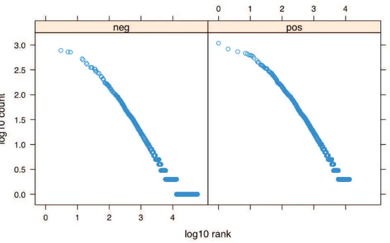
Online learning algorithms are typically used as blackboxes in NLP, without consideration of the peculiarities of natural language. Feature representations of text for tasks from spam filtering to parsing need to capture the variety of words, word combinations, and word attributes in the text, yielding very high-dimensional feature vectors, even though most of the features are absent in most texts. Nevertheless, those many rare features are very informative about the examples that contain them; indeed, features that occur frequently are typically less informative, hence the common use of stop-lists of frequent words such as function words, and of tf-idf term weighting.1 In Figure 1, we show the most predictive features for a simple NLP classification task and their frequency in data. Notice that while some predictive features are very common, most are relatively rare, indicating that modeling even infrequent features may be useful for learning. Therefore, it is worth investigating whether learning algorithms for linear classifiers could be improved to take advantage of these particularities of natural language data.

The foregoing motivation led us to proposeconfidence-weighted(CW) learning, a class of online learning methods that maintain a probabilistic measure of confidence in each weight. Less confident weights are updated more aggressively than more confident ones. Weight confidence is formalized with a Gaussian distribution over weight vectors, which is updated for each new training example so that the probability of correct classification for that example under the updated distribution meets a specified confidence. The result is an algorithm with superior classification accuracy over state-of-the-art online and batch baselines, faster learning, and new classifier combination methods for parallel training.

While our motivation for CW learning is from observations about NLP problems, the approach makes no assumptions about the input space and can be applied to other machine learning problems (Ma et al., 2009).

This paper brings together two types of confidence-weighted algorithms originally introduced by Dredze et al. (2008) and Crammer et al. (2008). In addition to a unified presentation, we include alternative formulations of the diagonal covariance algorithms along with empirical results. We also include further empirical evidence of the strength of these methods and an analysis of algorithmic behavior on NLP problems.

Figure 1: The top quartile of negative (left) and positive (right) features as ranked by mutual infor-mation with the label for sentiment data (described in Section 7). The x-axis is their (log) rank by mutual information and the y-axis is their total (log) count in the data. While some very frequent features are useful for predicting the label (high on the curve) there are a large number of low frequency features (low on the curve) that are still useful for learning. A sparse model would likely remove these low frequency features despite their predictive value.

We begin with a discussion of the motivating particularities of natural language data. We then introduce the confidence-weighted framework. From this framework we derive two types of al-gorithm following different formulations of the main constraint, each with a full covariance and several diagonalized versions. A series of experiments shows CW learning’s empirical benefits and an analysis reveals how algorithmic properties manifest themselves empirically. We conclude with a discussion of related work.

2. Characteristics of NLP Data

dimensional vector where only a small fraction of elements is nonzero, and feature frequencies have a heavy-tailed distribution (Figure 1).

Online algorithms do well with large numbers of features and examples, but they are not de-signed specifically for very sparse examples with a heavy-tailed feature frequency distribution. This can have a detrimental effect on learning. Typical linear classifier training algorithms update the weights of binary features only when they occur. The result is many updates for frequent features and few updates for rare features. Similarly, features that occur early in the data stream take more responsibility for correct prediction than those observed later. The result is a model that could have good weight estimates for common features but inaccurate weights for the great majority of features, which occur relatively rarely.

An illustrative case arises in sentiment classification. In this task, a product review is represented as n-grams and the goal is to label the review as being positive or negative about the product. Consider a positive review that simply read“I liked this author.” An online update would increase the weight of both “liked” and “author.” Since both are common words, over several examples the algorithm would converge to the correct values, a positive weight for “liked” and zero weight for “author.” Now consider a slightly modified negative example: “I liked this author, but found the book dull.”Since “dull” is a rare feature, the algorithm has a poor estimate of its weight. An update would decrease the weight of both “liked” and “dull.” The algorithm does not know that “dull” is rare and the changed behavior is likely caused by the poorly estimated rare feature (“dull”) instead of the well estimated common feature (“liked.”) An algorithm that maintains no information about the relative frequency or of second order information about features would attribute equal negative weight to both “liked” and “dull”, which slows convergence.

This example demonstrates how a lack of memory for previous examples—a property that al-lows online learning—can hurt learning. A simple solution is to augment an online algorithm with additional information, a memory of past examples. Specifically, the algorithm can maintain a con-fidence value for each feature weight. For example, assuming binary features, the algorithm could keep a count of the number of times each feature has been observed or how many times each weight has been updated. The larger the count, the more confidence we have in the weight of that feature. These estimates are then used to influence weight updates. Instead of equally updating every feature weight for the on-features of an example, the update favors changing low-confidence weights more aggressively than high-confidence ones. At each update, the confidence in the weights of observed features is increased, which will focus the update on the low confidence weights. In the example above, the update would decrease the weight of “dull” but make only a small change to “liked” since the algorithm already has a good estimate of this weight.

In the next section, we use this motivation from language data to present a new family of learning algorithms that associate a confidence value with each weight. For now, we wish to dispel two potential misinterpretations of the preceding very informal argument. First, while our approach is motivated by learning with sparse binary features with a heavy-tailed frequency distribution, the algorithms do not depend on those assumptions. Second, our notion of weight confidence is based on a probabilistic interpretation of passive-aggressive online learning, which differs from the more familiar Bayesian learning for linear classifiers. Nevertheless, analogously to Bayesian learning, it can be used to provide a useful notion of prediction confidence through a margin distribution (Dredze and Crammer, 2008a,b; Dredze et al., 2010).

xi Example on roundi

ˆ

yi Prediction on roundi

yi Label on roundi

wi Weight vector on roundi

µ_i The mean of the distribution on roundi

Σi The covariance matrix of the distribution on roundi

mi Margin on roundi

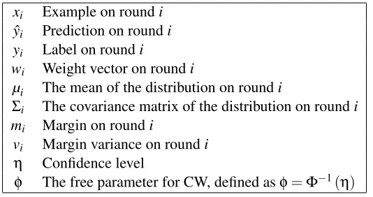
vi Margin variance on roundi η Confidence level

φ The free parameter for CW, defined asφ=Φ−1_(η)

Table 1: A reference table for notation used throughout the paper.

3. Online Learning of Linear Classifiers

Online algorithms operate in rounds, where each round corresponds to a single example. On round ithe algorithm receives an examplexi∈Rd to which it applies its current prediction rule to produce

a prediction ˆyi∈ {−1,+1}(for binary classification). It then receives the true labelyi∈ {−1,+1}

and suffers a lossℓ(yi,yˆi), which in this work will be the zero-one loss: ℓ(yi,yˆi) =1 ifyi 6=yˆiand ℓ(yi,yˆi) =0 otherwise. The algorithm then updates its prediction rule and proceeds to the next

round. For online evaluations, error is reported as the total lossℓon the training data and in batch evaluations, error is reported on held out data.

As is common in linear classification, our prediction rules are linear threshold functions fw(x):fw(x) =sign(x·w).

Two functions fwand fcware the same for non-negativec. Thus, we can identify fwwithw, which

we will do in what follows.

The signed marginof an example(x,y)with respect to a specific classifierwis defined to be y(w_·x). The sign of the margin is positive iff the classifier w correctly predicts the true label y. The absolute value of the margin _|y(w_·x)_|=_|w_·x_|can be thought of as the confidence2 in the prediction, with larger positive values corresponding to more confident correct predictions. We denote the margin at roundibymi=yi(wi·xi).

A variety of linear classifier training algorithms, including the perceptron and linear support vector machines, restrictwto be a linear combination of the input examples. Online algorithms of that kind typically have updates of the form

wi+1=wi+αiyixi , (1)

for some non-negative coefficientsαi.

In this paper we focus on passive-aggressive (PA) updates (Crammer et al., 2006a) for linear classifiers. After predicting withwi on the ithround and receiving the true labelyi, the algorithm

updates the prediction function such that the example(xi,yi)will be classified correctly with a fixed

margin (which can always be scaled to 1): wi+1=min

w

1

2kwi−wk 2

s.t. yi(w·xi)≥1. (2)

The general form of this problem is to enforce some learning constraints, in this case a prediction margin on the example, while minimizing the divergence to the current weights, which are assumed to be good since they encapsulate all previously observed examples. Solving this problem leads to an update of the form given by (1) with coefficientαidefined on each round as:

αi=

max_{1₋yi(wi·xi),0}

kxik2

, (3)

Like the perceptron, this is a mistake driven update, wherebyαi>0 iff the learning condition was

not met, ie. the example was not classified with a margin of at least 1. Note that the numerator of (3) is the hinge loss, which is zero only if the example is classified with a margin of 1. In practice, slack variables are introduced for non-separable data, restricting (3) as max_{αi,C}, for some free

parameterC.

Crammer et al. (2006a) provide a theoretical analysis of algorithms of this form, which have been shown to work well in a variety of applications (McDonald et al., 2004, 2005a; Chiang et al., 2008).

4. Distributions over Classifiers

Following the motivation of Section 2, we need a notion of confidence for the weight vector w maintained by an online learner for linear classifiers. Before any examples are seen, all of the weights in w are equally uncertain. As examples are observed, the confidence in the weights of features that are often active should increase faster than the confidence in the weights of rarely seen features.

Our concrete implementation of this idea is to represent the state of the learner with a probabil-ity densprobabil-ity overw, specifically a Gaussian distribution

N

featurep. The smallerΣp,p, the more confidence we have in the mean weight valueµp. Each

covari-ance termΣp,p′ captures our knowledge of the interaction between featurespandp′. The Gaussian

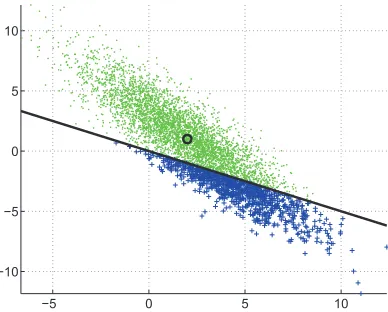
distribution naturally matches our intuition for confidence, as the covariance of the distribution is inversely proportional to our confidence: the smaller the determinant of the covariance, the less we expect the true weight value to deviate from the current estimate. This Gaussian representation is illustrated in Figure 2, which shows a Gaussian distribution over two-dimensional weight vectors. The black line represents an examplex= (0.5,1),y= +1, which divides the space between clas-sifiers that correctly classify this point (blue crosses below) and those that classify it incorrectly (green dots above).

In the CW model, the traditional signed marginy(w_·x)becomes a univariate Gaussian random variableM, where the mean of the distribution is the signed margin,

M_∼

N

−5 0 5 10 −10

−5 0 5 10

Figure 2: Gaussian distribution over two-dimensional weight vectors. Points above the black line (green dots) incorrectly classify the example((0.5,1),+1)and points below the line (blue crosses) classify it correctly. The density around a point is proportional to its relative weight. The black circle marks the mean of the Gaussian.

There are several ways to make predictions in this framework. A Gibbs predictor samples from the distribution a single weight vectorw, which is equivalent to drawing a margin value using (4), and takes its sign as the prediction. Other alternatives use averaging rather than sampling. For example, we can use the average weight vector E[w] =µ, as is done in Bayes point machines (Her-brich et al., 2001), which use a single weight vector to approximate a distribution. Alternatively, we can use the average margin E[M]. These two approaches are equivalent by linearity of expectation, E[w_·x] =µ_·x. Another approach estimates E[sign(M)]from many draws ofwfor fixedµ,Σ, and x. Since the sign function attains only two values (₋1 or+1) this is equivalent to computing the probability of acorrectprediction (not a large margin prediction), given by

Pr[M_≥0] =Pr_w∼N(µ,Σ)[y(w·x)≥0].

When possible we omit the explicit dependence on the distribution parameters and simply write Pr[y(w_·x)_≥0]. If the probability is larger than half, then the (weighted) majority votes fory= +1, otherwise, fory=₋1. Note that from the discussion below this prediction rule is equivalent to the previous two. Conceptually, it is useful to think of prediction as drawing a weight vectorwfrom the distribution, ie.w_∼

N

5. Learning Confidence-Weighted Classifiers

CW is an online learning algorithm, so on roundithe algorithm receives examplexifor which

it issues a prediction ˆyi.3 The algorithm predicts ˆyias sign(µi·xi), which is equivalent to averaging

the predictions of many sampled weight vectors from the distribution. On being presented with the labelyi, the algorithm adjusts the distribution to enforce a learning condition. Following the intuition

underlying the PA algorithms of Crammer et al. (2006a), we require that an update achieves both a large margin on the example and minimizes the change in weights. In this case, a large prediction margin is formalized as ensuring that the probability of a correct prediction for training examplei is no smaller than the confidence levelη_∈[0,1]:

Pr[yi(w·xi)≥0]≥η.

Minimization of weight changed is enforced by finding a new distribution closest in the KL di-vergence4sense to the current distribution

N

distribution by solving the following optimization problem:

(µ_i+1,Σi+1) =min DKL(

N

N

s.t. Pr[yi(w·xi)≥0]≥η. (6)

This update can be understood as a probabilistic counterpart of the PA objective (2).

We now develop both the objective and the constraint of this optimization problem following Boyd and Vandenberghe (2004, page 158). We start with the objective (5) and write the KL diver-gence between two Gaussians as

DKL(

N

N

log

detΣ1 detΣ0

+Tr Σ−1 1 Σ0

+ (µ1−µ0)⊤Σ1−1(µ1−µ0)−d

.

We now proceed with the constraint in (6). As noted above, under the distribution

N

mi=yi(µi·xi) , (7)

and variance

σ2_i =vi=x⊤i Σixi. (8)

Thus the probability of awrongclassification is

Pr[M_≤0] =Pr

M₋m

σ ≤

−m

σ

.

Since(M₋m)/σis a normally distributed random variable, the above probability equalsΦ(₋m/σ), where

Φ(u) = √1 2π

Z u

−∞e

−v2 dv,

3. For a related batch formulation of CW learning, see recent work of Crammer et al. (2009b).

4. DKL(p(x)kq(x)) =Rp(x)log

_p(x)

q(x)

is the cumulative Gaussian distribution. Thus we can rewrite (6) as −m

σ ≤Φ−

1₍₁

−η) =₋Φ−1(η) .

Substitutingmandσby their definitions and rearranging terms we obtain yi(µ·xi)≥φ

q

x⊤_i Σxi,

whereφ=Φ−1_{(η). To conclude the update rule solves the following optimization problem:}

(µ_i+1,Σi+1) =arg min

µ,Σ

1 2log

detΣi

detΣ

+1

2Tr Σ −1

i Σ

+1

2(µi−µ) ⊤_Σ−1

i (µi−µ)

s.t.yi(µ·xi)≥φ q

x⊤_i Σxi . (9)

Conceptually, this is a large-margin constraint, where the value of the margin requirement depends on the examplexivia a quadratic form.

Unfortunately, this constraint is not convex in Σsince the term

q

x⊤_i Σxi is concave in Σ. We

propose two alternatives to obtain a convex constraint: linearization (Section 5.1) and change of variables (Section 5.2). Additionally, we propose few alternatives to solve the learning optimization problem restricted todiagonalmatrices in Section 6.

5.1 Linearization of the Constraint

In out first approach to obtain a convex problem we simply linearize the constraint of (9) by omitting the square root to obtain the revised optimization problem.

(µ_i+1,Σi+1) =arg min 1 2log detΣi detΣ +1

2Tr Σ −1

i Σ

+1

2(µi−µ) ⊤_Σ−1

i (µi−µ)

s.t.yi(µ·xi)≥φ

x⊤_i Σxi

. (10)

We call this formulationvar, since we have replaced the standard deviation in the constraint with the variance. This formulation was introduced by Dredze et al. (2008). The following lemma summarizes the solution of this formulation,

Lemma 1 The optimal solution of this form is,

µ_i+1=µ_i+αyiΣixi Σ−_i+1₁=Σ_i−1+2αφxix⊤i ,

where the value of the parameterα(a Lagrange multiplier) is given by

αi=max







0,−(1+2φmi) + q

(1+2φmi)2−8φ(mi−φvi)

4φvi





 .

where mi=yi(µi·xi)(see(7)) and vi=x⊤i Σixi (see(8)).

The derivation appears in Section 5.1.1 below. The resulting algorithm is shown in Figure 1, where the update uses (11) and (13) to update the distribution with coefficients βi ((15)) and αi

Algorithm 1Binary CW Online Algorithm. The two versions of the Confidence-Weighted algo-rithm: (1) linearization and (2) change of variables. The numbers in parentheses refer to equations in the text, where more detail can be found.

Input:η_∈[0.5,1] Initialize:

µ₁=0,Σ1=I,

φ=Φ−1_{(η), φ}′_=1+φ2_{/2, φ}′′_=1+φ2_.

fori=1,2. . . do

Receive a training examplexi∈Rd

Compute Gaussian margin distributionmi∼

N

Receive true labelyi

Suffer lossℓi=1 iffyiE[sign(mi)]≤0

Compute Update:

• Define: mi=yi(µi·xi) (7) vi=x⊤i Σixi (8)

• Linearization:

αi=max







0,−(1+2φmi) + q

(1+2φmi)2−8φ(mi−φvi)

4φvi







(18)

βi=

2αiφ

1+2αφvi

(15)

• Change of Variables:

v+_i =





−αviφ+

q α2_v2

iφ2+4vi

2





2

(28)

αi=max 





0,−miφ

′₊q_m2

i

φ4

4 +viφ2φ′′ viφ′′







(31)

βi=

αiφ q

v+_i +viαiφ

(27)

Update

µ_i+1=µ_i+αiyiΣixi (11,20) Σi+1=Σi−βiΣixix⊤i Σi (14,25) end for

5.1.1 DERIVATION OFLEMMA1

The optimization objective is convex inµandΣsimultaneously and the constraint became linear, so any convex optimization solver van be used to solve this problem. The Lagrangian for this optimization is

L

2log

detΣi

detΣ

+1

2Tr Σ −1

i Σ

+1

2(µi−µ) ⊤_Σ−1

i (µi−µ)

+α₋yi(µ·xi) +φ

x⊤_i Σxi

.

Taking partial derivatives, we know that at the optimum, we must have

∂ ∂µ

L

−1

i (µ−µi)−αyixi=0.

AssumingΣiis non-singular and rearranging terms we get

µ_i+1=µ_i+αyiΣixi. (11)

At the optimum, we must also have

∂

∂Σ

L

1 2Σ

−1₊1 2Σ

−1

i +φαxix⊤i =0, (12)

and solving forΣ−1_{we obtain}

Σ−1

i+1=Σ−i 1+2αφxix⊤i . (13)

Before proceeding, we observe that (13) computes Σ−_i+1₁ as the sum of a rank-one positive semi-definite (PSD) matrix andΣ−_i 1 . Thus, ifΣ−_i 1is PSD, so are Σ−_i+1₁ andΣi+1 thusΣi is indeed

non-singular, as assumed above. The update guarantees that the eigenvalues of the inverse-covariance matrix always increase.

Finally, we compute the inverse of (13) using the Woodbury identity (Petersen and Pedersen, 2008, Equation 135) and get

Σi+1=

Σ−_i 1+2αφxix⊤i −1

=Σi₋Σixi

1 2αφ+x

⊤

i Σixi −1

x⊤_i Σi

=Σi−Σixi

2αφ

1+2αφvi

x⊤_i Σi

=Σi−βiΣixix⊤i Σi, (14)

where

vi = x⊤i Σixi

βi =

2αφ

1+2αφvi

The KKT conditions for the optimization imply that the eitherα=0, and no update is needed, or the constraint in (10) is an equality after the update. Substituting (11) and (14) into the equality version of (10), we obtain

yi(xi·(µi+αyiΣixi)) =φ

x⊤_i Σi−Σixiβix⊤i Σi

xi

. (16)

Rearranging terms we get

yi(xi·µi) +αx⊤i Σixi=φx⊤i Σixi−φv2iβi. (17)

Substituting (7), (8), and (15) into (17) we obtain

mi+αvi=φvi−φv2i

2αφ

1+2αφvi .

We multiply both sides by 1+2αφviand get

(mi+αvi) (1+2αφvi) =φvi(1+2αφvi)−2αφ2v2i .

Rearranging the terms we obtain,

0 = mi+αvi+2αφvimi+2α2φv2i −φvi = α2 2φv2_i+αvi(1+2φmi) + (mi−φvi) .

The above equality is a quadratic equation inα. Its smaller root is always negative and thus is not a valid Lagrange multiplier. Letγibe its larger root:

γi=

−(1+2φmi) + q

(1+2φmi)2−8φ(mi−φvi)

4φvi

. (18)

The constraint (10) is satisfied before the update ifmi−φvi≥0. If 1+2φmi≤0, thenmi≤φviand

from (18) we have thatγi>0. If, instead, 1+2φmi≥0, then, again by (18), we have γi>0

⇔

q

(1+2φmi)2−8φ(mi−φvi)>(1+2φmi)

⇔mi<φvi .

From the KKT conditions, eitherαi =0 or (10) is satisfied as an equality. In the later case, (16)

holds, and thusαi=γi>0, which concludes the derivation of the lemma.

5.2 Change of Variables

SinceΣis positive-semidefinite (PSD) it can be written as the square of another PSD matrix5_ϒ:

Σ=ϒ2 , ϒ=√Σ.

Substituting in (9) gives the revised optimization problem

(µ_i+1,ϒi+1) =arg min 1 2log

detϒ2

i

detϒ2

+1

2Tr ϒ −2

i ϒ

2

+1

2(µi−µ) ⊤_ϒ−2

i (µi−µ)

s.t. yi(µ·xi)≥φkϒxik

ϒis PSD. (19)

Note that, the objective is convex since₋log detϒ2_{=−2 log detϒwhich is well defined sinceϒis} PSD. The constraint is a second-order cone inequality and therefore convex.

We call this formulation stdev, since we have maintained the standard deviation in the con-straint. This formulation was introduced by Crammer et al. (2008).

Standard optimization techniques can solve the convex program (19), but these methods can be slow. Instead, as before we derive a closed-form solution which we summarize in the following lemma:

Lemma 2 The optimal solution of this form is,

µ_i+1=µ_i+αyiΣixi Σi+1=Σi−βΣixix⊤i Σi,

where

β= q αφ

v+_i +viαφ

, v+_i =x⊤_i Σi+1xi.

and the value of the parameterα(a Lagrange multiplier) is given by

α=max







0,1

vi

−miφ′+ q

m2

i

φ4

4 +viφ2φ′′

φ′′





 .

where mi=yi(µi·xi)(see(7)), vi=x⊤i Σixi(see(8)), and for simplicity we defineφ′=1+φ2/2,φ′′=

1+φ2_.

The resulting algorithm is shown in Figure 1. 5.2.1 DERIVATION OFLEMMA2

The Lagrangian for (19) is

L

2log

detϒ2

i

detϒ2

+1

2Tr ϒ −2

i ϒ2

+1

2(µi−µ) ⊤_ϒ−2

i (µi−µ) +α(−yi(µ·xi) +φkϒxik) .

At the optimum, it must be that

∂ ∂µ

L

−2

i (µ−µi)−αyixi=0.

Therefore, ifϒiis non-singular, the update for the mean is

µ_i+1=µ_i+αyiϒ2ixi. (20)

At the optimum, we must also have

∂

∂ϒ

L

−1₊1 2ϒ

−2

i ϒ+

1 2ϒϒ

−2

i +αφ

xix⊤i ϒ

2

q

x⊤_i ϒ2_x

i

+αφ ϒxix⊤i

2

q

x⊤_i ϒ2_x

i

=0. (21)

Defining the matrix

C=ϒ−_i 2+αφqxix⊤i

x⊤_i ϒ2_x

i

, (22)

we get

∂

∂ϒ

L

−1₊1 2ϒC+

1

2Cϒ=0 at the optimum. From this, it follows easily that at the optimum

ϒ=C−12 .

Substituting (22) into this equation, we obtain the update

ϒ_i−₊2₁=ϒ_i−2+αφq xix⊤i

x⊤_i ϒ2

i+1xi .

Conveniently, the final form of the updates can be expressed in terms of the covariance matrix:6 µ_i+1 = µ_i+αyiΣixi (23) Σ_i−₊1₁ = Σ_i−1+αφq xix⊤i

x⊤_i Σi+1xi

. (24)

As before we observe that if Σ−_i 1 is PSD, so are Σ_i−₊1₁ and Σi+1 with monotonically decreasing eigenvalues. ThusΣiis indeed non-singular, as assumed above.

It remains to determine the value of the Lagrange multiplier α. As before we compute the inverse of (24) using the Woodbury identity (Petersen and Pedersen, 2008) to get,

Σi+1 =



Σ−_i 1+αφ

xix⊤i q

x⊤_i Σi+1xi 



−1

= Σi₋Σixi 

 q

x⊤_i Σi+1xi αφ +x

⊤

i Σixi 



−1 x⊤_i Σi

= Σi₋Σixi 



αφ q

x⊤_i Σi+1xi+x⊤i Σixiαφ 

x⊤_i Σi

= Σi−βiΣixix⊤i Σi. (25)

where we define

v+_i =x⊤_i Σi+1xi, (26)

and

βi=

αiφ q

v+_i +viαiφ

. (27)

Multiplying (25) byx⊤_i (left) andxi (right) we get

v+_i =vi−vi 



αφ q

v+_i +viαφ 

v_i ,

which is equivalent to

v+_i

q

v+_i +v+_i viαφ = vi q

v+_i +v2_iαφ₋v2_iαφ = vi

q

v+_i .

Dividing both sides by

q

v+_i , we obtain

v+_i +

q

v+_i viαφ−vi=0,

which can be solved forv+_i to obtain

q

v+_i =−αviφ+

q α2_v2

iφ2+4vi

2 . (28)

Using the equality version of (19) and Equations (23,25,26,28) we obtain

mi+αvi=φ

−αviφ+ q

α2_v2

iφ2+4vi

2 , (29)

which can be rearranged into the following quadratic equation inα:

α2_v2

i 1+φ2

+2αmivi

1+φ

2 2

+ m2_{i −}viφ2

=0.

The smaller root of this equation is always negative and thus not a valid Lagrange multiplier. We use the following abbreviations for writing the larger rootγi,

φ′=1+φ2/2 ; φ′′=1+φ2.

The larger root is then

γi=−mivi

φ′₊q_m2

iv2iφ′2−vi2φ′′ m2i −viφ2

v2_iφ′′ . (30)

The constraint (19) is satisfied before the update ifmi−φ√vi≥0. Ifmi≤0, then mi≤φ√viand

from (30) we have thatγi>0. If insteadmi≥0, then, again by (30), we have γi>0

⇔miviφ′< q

m2_iv2_iφ′2_−v2

iφ′ m2i −viφ2

⇔mi<φvi .

From the KKT conditions, eitherαi=0 or (10) is satisfied as an equality, so (29) holds andαi= γi>0.

The solution of (30) satisfies the KKT conditions, that is eitherαi≥0 or the constraint of (10) is

satisfied before the update with the weightsµ_iandΣi. We obtain the final form ofαiby simplifying

(30) together with last comment and get,

αi=max







0,1

vi

−miφ′+ q

m2

i

φ4

4 +viφ2φ′′

φ′′







. (31)

6. Diagonal Covariance Matrices

So far we have said nothing about the covariance matrixΣ, which grows quadratically in the number of features. Since our intended applications are NLP tasks, computing the full matrixΣis computa-tionally infeasible. Addicomputa-tionally, even though we initialize the matrix to be diagonal (Figure 1), after applying the updates rule of either (14) (linearization/var) or (25) (change of variables/stdev), we may obtain a full covariance matrix, as we subtract fromΣi a rank-one matrix proportional to the

In this section, we reduce the size of Σby restriction to a diagonal-covariance matrix.7 _We discuss two main approaches, each of which can be applied to either the linearization or the change of variables formulations. In Section 6.1 we show two ways to use the full-covariance updates discussed above and add a diagonalization step. In Section 6.2 we take an alternative approach and re-develop the update step assuming an explicit diagonal representation of the covariance matrix.

6.1 Approximate Diagonal Update

Both updates above (linearization or change-of-variables) share the same form when updating the covariance matrix ((14) or (25))

Σi+1=Σi−βiΣixix⊤i Σi. (32)

Our diagonalization step will define the final matrix to be a diagonal matrix with its non-zero ele-ments equals to the diagonal eleele-ments of (32). Formally we get,

Σi+1 = diag

Σi₋βiΣixix⊤i Σi

= diag(Σi)−diag

βiΣixix⊤i Σi

= Σi−βidiag

Σixix⊤i Σi

,

where the last equality follows since we assume thatΣiis diagonal and

diag(A) =

Ap,p′ p=p′

0 p₆=p′ .

A na¨ıve implementation of the diagonal operator takes Θ(d2) time and space. An efficient implementation first defineszi=Σixiand then sets,

Σi+1

p,p=

Σi

p,p−βi

zi

p 2

for p=1, . . . ,d.

We refer to this diagonalization scheme asL2since it is equivalent to a projection of the full matrix onto the set of diagonal matrices using the Euclidean norm.

We note in passing that since the diagonalization operator and the inverse operator arenot com-mutative, we can first diagonalize the inverse of the covariance matrix and then invert the result. Concretely we start from the update of the inverse-covariance,

Σ_i−₊1₁=Σ_i−1+ηixix⊤i ,

where

ηi=2αiφ,

for the linearization approach ( (13) ) and

ηi= q αiφ

x⊤_i Σi+1xi ,

for the change of variables approach ((24)). We first diagonalize the inverse-covariance and get

Σ−1

i+1 = diag

Σ−1

i +ηixix⊤i

= diag Σ−_i 1

+diag

ηixix⊤i

= Σ−1

i +ηidiag

xix⊤i

.

As before we implement the update efficiently by writing

Σ−_i+1₁

p,p=

Σ−_i 1 p,p+ηi

xi

p 2

for p=1, . . . ,d,

or in terms of the covariance matrix

Σi+1

p,p= 1 1 Σi

p,p +ηi xi p

2 for p=1, . . . ,d.

We refer to this diagonalization scheme as KL since it is equivalent to a projection of the full matrix onto the set of diagonal matrices using the Kullback-Leibler (KL) divergence.

6.2 Exact Diagonal Update

An alternative to the approximate formulation is to explicitly maintain a diagonal and develop a corresponding update. We now assume that the matrixΣis diagonal. We denote by Σi,(p)the rth

diagonal element of the matrixΣi, and byxi,(p)the rthelement ofxi. We start with the first alternative

above where we used linearization. We follow the derivation of Section 5.1 until (11). Proceeding with derivation of (12), but only for the diagonal elements indexed bypwe get,

∂

∂Σ_(p)

L

1 2Σ_(p)+

1

2Σ_i,(p)+φαx

2

i,(p)=0 for p=1, . . . ,d,

Solving forΣ(p)we get

Σi+1,(p)=

Σ_i,(p)

1+2αΣi,(p)φx2_i,(p)

.

Following the logic presented after (15) we get that at the optimum we have

yi(xi·(µi+αyiΣixi)) =φ

∑

x2_i,(p) Σi,(p) 1+2αΣ_i,(p)φx2i,(p)

.

Substituting (7) and (8) and rearranging the terms we get the constraint f(α) =0,

where we defined

f(α) =mi+αvi−

∑

Σ_i,(p)φx2_i,(p) 1+2αΣ_i,(p)φx2

i,(p)

We will analyze (33) after developing its equivalent for the second alternative above where we perform a change of variables. As above we denote byϒi,(p)the rthdiagonal element of the matrix

ϒi. We follow the derivation of Section 5.2 until (20). Proceeding with derivation of (21), but only

for the diagonal elements indexed byrwe get

∂ ∂ϒ(p)

L

x2_i,(p)ϒ(p)

q

x⊤_i ϒ2_x

i =0.

Rearranging the terms we get

1

ϒ2

(p)

= 1

ϒ2

i,(p)

+αφ x

2

i,(p)

q

x⊤_i ϒ2_x

i .

Thus,

ϒ2_(p)= ϒ

2

i,(p)

q

x⊤_i ϒ2_x

i

q

x⊤_i ϒ2_x

i+αφx2_i,(p)ϒ2_i,(p) .

Multiplying both sides byx2_i,(p)and summing overrwe get

x⊤_i ϒ2xi=

∑

x2_i,(p)ϒ2_(p)=

q

x⊤_i ϒ2_x

i

∑

x2_i,(p)ϒ2

i,(p)

q

x⊤_i ϒ2_x

i+αφx2_i,(p)ϒ2_i,(p) .

Finally, we obtain

q

x⊤_i ϒ2_x

i=

∑

x2_i,(p)ϒ2

i,(p)

q

x⊤_i ϒ2_x

i+αφx2_i,(p)ϒ2_i,(p) .

As before we employ the KKT conditions which state that whenα>0 we have mi+αvi=φ

q

x⊤_i ϒ2_x

i.

Substituting in the last equality we get

q

x⊤_i ϒ2_x

i=

∑

φx2_i,(p)ϒ2

i,(p)

mi+αvi+αφ2x2_i,(p)ϒ2_i,(p) .

We use again the KKT conditions and get that the optimal valueαi+1is the solution ofg(α) =0 for g(α) =mi+αvi−

∑

r

φ2_x2

i,(p)ϒ2i,(p)

mi+αvi+αφ2x2_i,(p)ϒ2_i,(p)

. (34)

The functiong(α)defined in (34) and the function f(α)defined in (33) are both of the form h(α) =mi+αvi−

∑

r

ar

b+crα ,

wherevi,ar,cr≥0. The only difference is thatb=1>0 in (33) andb=mi in (34). Nevertheless,

Lemma 3 Assume that vi>0and let Li=max{0,−mi/vi}. Both(33)and(34)have the following

properties:

1. Their value at Liis non-positive, that is f(Li)≤0,g(Li)≤0.

2. They are strictly-increasing forα_≥Li

3. For each function there exists a value Ui such that their value at Ui is positive, f(Ui)>

0,g(Ui)>0

Proof For the first property we consider two casesmi≥0 andmi<0. We start with the first case

and thusLi=0. Thus, f(0) =mi−∑rΣi,(p)φx2i,(p)=mi−φvi<0, where the last ineqluaity follows

since we assume that the constraint of (10) does not hold. Also,g(0) =mi−_m1_i∑rφ2x2i,(p)ϒ2i,(p)=

mi−φ2_mvi_i <0 since we assumed that the constraint of (19) does not hold. Whenmi <0 we have

Li=−mi/vi>0. In this case (33) becomes,

f(Li) =−

∑

Σ_i,(p)φx2_i,(p) 1+2LiΣi,(p)φx2i,(p)

≤0,

sinceΣ_i,(p)φx2i,(p)≥0. Similarly,

g(Li) =−

∑

φ2_x2

i,(p)ϒ2i,(p)

Liφ2_x2

i,(p)ϒ2i,(p)

=₋d

Li <0.

The second property of strictly-increasing follows immediately since vi >0 and since for both

functions the denominator of each term in the sum over p is an increasing function in α which is non-negative in the range α_≥Li. Finally, the last property follows directly from the second

property.

The lemma states that for each of fandgthere is exactly oneαi(possibly different for each function)

such that f(αi) =0 andg(αi) =0, but it does not provide an expression for computingαiexplicitly such as in Lemma 1. However, it further tells us that for each function the value of αi is in the

interval[Li,Ui]. A value not far fromαi up to an accuracy ofεcan be found using binary search in

time proportional to[(Ui−Li)log(1/ε)].

We conclude this section by computing a possible valueUifor each function and start with (33).

Note thatai=max{0,−2mi/vi}satisfiesmi+(ai/2)vi≥0. Thus,bi=maxr n

2dΣi,(p)φx2_i,(p)

/vi

o

satisfiesbivi/(2d)−Σi,(p)φx2_i,(p)/

1+2αΣi,(p)φx2_i,(p)

≥0 for p=1. . .d. Therefore settingUi=

max_{ai,bi}satisfies f(Ui)≥0 as desired. Finally, note thatUi≥Li sinceai≥Li by construction.

For (34) we use the same definition of ai but define bi=maxr n

2dϒ2

i,(p)φ2x2i,(p)

/vi

o

andUi=

max_{ai,bi}. By a similar argument we haveg(Ui)>0 andLi≤Ui.

7. Evaluation

In this section we evaluate diagonalized versions of the CW algorithm on a range of binary classifi-cation problems for NLP tasks. We compare our methods against each other and against competitive online and batch learning algorithms.

We selected a range of 5 tasks and created 17 binary classification problems. We begin with a description of each task.

7.1 20 Newsgroups

The 20 Newsgroups corpus contains approximately 20,000 newsgroup messages, partitioned across 20 different newsgroups.8 The data set is a popular choice for binary and multi-class text classifi-cation as well as unsupervised clustering. Following common practice, we created binary problems from the data set by creating binary decision problems of choosing between two similar groups. Our groups are:

• comp:comp.sys.ibm.pc.hardwarevs.comp.sys.mac.hardware

• sci:sci.electronicsvs.sci.med

• talktalk.politics.gunsvs.talk.politics.mideast

Each message was represented as a binary bag-of-words. For each problem we selected 1800 ex-amples balanced between the two labels.

7.2 Reuters

The Reuters Corpus Volume 1 (RCV1-v2/LYRL2004) contains over 800,000 manually categorized newswire stories (Lewis et al., 2004). Each article contains one or more labels describing its gen-eral topic, industry and region. We created the following binary decision tasks from the labeled documents:

• Insurance: Life (I82002) vs. Non-Life (I82003)

• Business Services: Banking (I81000) vs. Financial (I83000)

• Retail Distribution: Specialist Stores (I65400) vs. Mixed Retail (I65600).

These distinctions involve neighboring categories so they are fairly hard to make. Details on doc-ument preparation and feature extraction are given by Lewis et al. (2004). For each problem we selected 2000 examples using a bag-of-words representation with binary features. Each problem contains a balanced mixture of examples from each label.

7.3 Sentiment

We used a larger version of the sentiment multi-domain data set of Blitzer et al. (2007) used in Dredze et al. (2010).9 This data consists of product reviews from 7 Amazon domains (apparel, book, dvd, electronics, kitchen, music, video). The goal in each domain is to classify a product

review as either positive or negative. Feature extraction creates unigram and bigram features using counts following Blitzer et al. (2007). For the apparel domain we used all 1940 examples and for all other domains we used 2000 examples. Each problem contains a balanced mixture of example labels.

7.4 Spam

We include a spam classification problem as a sample problem from the space of email classification tasks. We chose spam since it is a widely studied problem with several publicly available data sets. We selected the 2006 ECML/PKDD Discovery Challenge spam data set (Bickel, 2006) and use the provided representations (bag-of-words). The goal is to classify an email (bag-of-words) as either spam or ham (not-spam). This corpus contains two data sets: task A, which has three users, and task B, which has 15 users. We use the three users from task A since it has more training examples. For each user we select 2000 examples.

7.5 Pascal

The PASCAL large scale learning challenge workshop provided several large scale binary data sets.10 We selected the NLP task, which is a Webspam filtering problem. Each example is the text from a web page. The task is to classify a webpage as either spam or ham. We used the default format provided by the workshop and selected 2000 examples.

7.6 USPS

The USPS data set contains examples of all 10 digits as part of a digit recognition task (OCR) (Hull, 1994). We created binary tasks by pairing each digit with another in order: 0/9, 1/2, 3/4, 5/6, 7/8. We used the standard value of each pixel in the image, as well as the product of all the pixel pairs in the image (bi-grams.)

Each data set was randomly divided for 10-fold cross validation experiments. Classifier param-eters (φ) and the number of training iterations (up to 10) were tuned for each classification task on a single randomized run over the data. Results are reported for each problem as the average accuracy over the 10 folds. Statistical significance is computed using McNemar’s test.

7.7 Results

We start by comparing the performance of the diagonalized CW algorithms: var (linearization) against stdev(change of variables), approximate against exact diagonalization, and for approxi-mate updates, KL againstL2. All six algorithm combinations were run on the data sets described above. The average test error on all data sets is shown in Table 2. For each method, we summarize its overall performance by computing its mean rank among all the other algorithm: if an algorithm has a mean rank of 1 then on average across all data sets it achieved the lowest error on average, whereas a rank of 6 indicates that it ranked 6th in error on average across all tests.

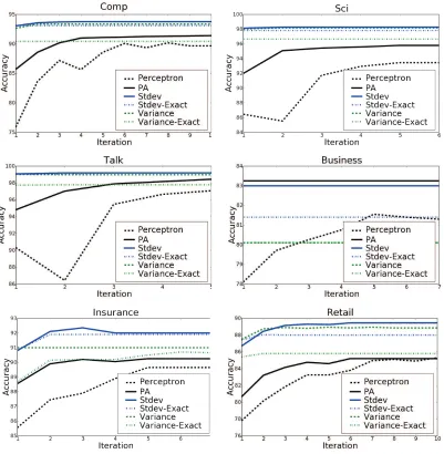
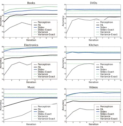
Figure 3: Accuracy on test data after each iteration on six data sets.

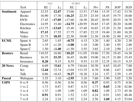
Figure 4: Accuracy on test data after each iteration on the six Amazon data sets.

We next compare the results from our approximation diagonalization CW methods to other pop-ular online learning algorithms (Table 3). We evaluated the perceptron (Rosenblatt, 1958), passive-aggressive (Crammer et al., 2006a), stochastic gradient descent (Zhang, 2004; Blitzer et al., 2007) and a diagonalized second order perceptron (Cesa-Bianchi et al., 2005), all of which perform well for NLP problems. In every experiment, a CW method improved over all of the online learning baselines.

var stdev

Task KL L2 Exact KL L2 Exact

Sentiment Apparel 12.53 12.47 14.79 13.66 13.51 14.28 Books 16.90 17.30 19.60 16.25 22.35 15.25

DVD 17.45 17.05 19.05 17.60 18.30 16.95

Electronics 14.95 15.40 16.65 14.75 20.95 15.50 Kitchen 13.75 13.65 15.30 15.40 15.40 14.25 Music 17.15 17.55 19.90 17.75 17.85 19.35 Video 21.75 18.55 25.85 22.50 19.00 23.60

ECML Spam A 2.65 1.45 3.10 0.75 4.15 0.80 Spam B 1.35 1.20 2.65 1.00 1.10 1.05 Spam C 1.50 1.40 3.40 1.50 3.55 1.35 Reuters Retail 10.55 18.80 18.75 10.25 11.05 11.05 Business 16.35 15.35 17.10 16.45 16.80 17.20 Insurance 8.20 9.15 10.20 8.55 9.55 10.10

20 News Comp 6.69 5.61 8.59 6.79 16.64 6.90 Sci 2.44 2.74 3.20 3.04 13.35 3.10 Talk 0.86 0.43 2.43 0.27 8.38 1.14

Pascal Webspam 3.55 3.10 3.85 2.95 3.10 5.35 Mean Rank 2.53 2.35 5.29 2.47 4.53 3.59

Table 2: Average Error of all variants of confidence-weighted algorithms presented in this paper over 17 binary text classification tasks. The best score for each data set is set in bold. The mean rank is the average rank of each algorithm across data sets, ranging from 1 (best) to 6.

seen in Figure 7.6 and Figure 7.6, which shows test error after each training iteration for CW and PA. While CW clearly improves over PA, it converges very quickly, reaching near best performance on the first iteration. In contrast, PA benefits from multiple iterations over the data; its performance changes significantly from the first to fifth iteration. The plot also illustrates exact’s behavior, which initially beats PA but does not improve. In fact, on eleven of the twelve data sets,var-Exact beats PA on the first iteration.

7.8 Batch Learning

While online algorithms are widely used, batch algorithms are still preferred for many tasks. Batch algorithms can make global learning decisions by examining the entire data set, an ability beyond online algorithms. In general, when batch algorithms can be applied they perform better. We compare CW to three standard batch algorithms: na¨ıve Bayes (default configuration in MALLET McCallum, 2002), maximum entropy classification (default configuration in MALLET McCallum, 2002) and support vector machines (LibSVM Chang and Lin, 2001). Classifier parameters (Gaus-sian prior for maxent andCfor SVM) were tuned as for the online methods.

var stdev

Task KL L2 KL L2 Per PA SOP SGD

Sentiment Apparel 12.53 12.47 13.66 13.51 17.84 13.35 17.42 13.76 Books 16.90 17.30 _∗16.25 22.35 23.10 18.45 19.75 18.60 DVD 17.45 _∗17.05 _∗17.60 18.30 20.45 20.95 20.55 18.70 Electronics 14.95 15.40 ⋆14.75 ⋆20.95 18.65 17.45 20.20 16.00 Kitchen ⋆13.75 _∗13.65 15.40 15.40 16.65 15.20 21.20 16.00 Music 17.15 17.55 17.75 17.85 22.35 19.40 21.80 18.20 Video 21.75 18.55 22.50 19.00 21.50 18.90 21.90 19.25

ECML Spam A 2.65 1.45 ⋆0.75 4.15 3.20 1.40 4.20 2.30 Spam B 1.35 ⋆1.20 _∗1.00 1.10 3.00 2.40 1.95 2.80 Spam C 1.50 ⋆1.40 ⋆1.50 3.55 3.65 2.10 2.90 2.15

Reuters Retail †10.55 18.80 †10.25 †11.05 19.60 17.50 19.45 14.30 Business 16.35 15.35 16.45 16.80 19.00 16.15 21.80 15.45 Insurance 8.20 9.15 8.55 9.55 11.35 12.35 10.15 9.35

20 News Comp 6.69 †5.61 6.79 †16.64 10.30 8.65 10.45 7.88 Sci †2.44 †2.74 _∗3.04 †13.35 6.70 8.06 4.67 4.06 Talk 0.86 _∗0.43 †0.27 †8.38 3.24 1.57 2.59 1.19

Pascal Webspam 3.55 3.10 ⋆2.95 3.10 7.60 3.90 5.05 3.50

USPS 0 vs 9 0.56 0.56 0.56 0.56 0.37 0.93 0.75 0.56 1 vs 2 1.73 0.87 0.87 4.33 1.73 0.65 2.38 42.86 3 vs 4 1.37 1.09 1.09 1.09 0.82 1.09 2.73 45.36 5 vs 6 0.91 0.91 1.52 1.52 4.24 0.91 3.03 48.48 7 vs 8 2.24 2.24 1.92 2.24 2.56 1.60 4.15 53.04 Table 3: Average Error of approximate-diagonal confidence-weighted algorithms and four other

online algorithms: The perceptron algorithm (Per), the passive-aggressive (PA) algorithm, the second order perceptron (SOP) and stochastic gradient decent evaluated using 17 bi-nary text classification tasks. The best score for each data set is set in bold. Statistical significance measured by McNemar’s test indicates when a CW algorithm is statistically significant (⋆p=0.05,_∗ p=0.01, † p=0.001) from each of the four baselines (percep-tron, PA, SOP, SGD).

algorithm beats all of the batch methods. The much faster and simpler online algorithm performs better than the slower more complex batch methods.

The speed advantage of online methods in the batch setting can be seen in Table 5, which shows the average training time in seconds for a single experiment (fold) for a representative selection of CW algorithms and some of the baselines. The online times include the multiple iterations selected for each online learning experiment. The differences between the online and batch algorithms are striking. While CW performs better than the batch methods, it is also much faster, while being equivalent in speed to the other online methods. For webspam data, which contains many features, an SVM takes over 1.5 minutes to train while the CW algorithms take between 1-2 seconds.

var stdev

Task KL L2 KL L2 NB Maxent SVM

Sentiment Apparel 12.53 12.47 13.66 13.51 12.63 13.56 13.92 Books 16.90 17.30 ⋆16.25 †22.35 18.40 18.05 18.25 DVD 17.45 17.05 17.60 18.30 21.00 18.00 19.60 Electronics 14.95 15.40 ⋆14.75 †20.95 17.05 15.85 16.25 Kitchen ⋆13.75 13.65 15.40 15.40 15.00 15.25 15.50 Music 17.15 17.55 17.75 17.85 18.65 17.90 18.25 Video 21.75 18.55 22.50 19.00 22.95 18.40 18.80

ECML Spam A ⋆2.65 1.45 ⋆0.75 4.15 3.70 1.30 1.75 Spam B 1.35 1.20 ⋆1.00 1.10 4.20 1.55 1.90 Spam C 1.50 1.40 1.50 †3.55 1.40 1.35 1.40

Reuters Retail _∗10.55 ⋆18.80 †10.25 _∗11.05 16.55 12.55 12.90 Business 16.35 15.35 16.45 16.80 20.00 15.85 15.60 Insurance 8.20 9.15 8.55 9.55 11.80 9.10 9.75

20 News Comp 6.69 5.61 6.79 †16.64 5.56 7.82 7.67

Sci ⋆2.44 ⋆2.74 3.04 †13.35 1.42 3.40 3.86 Talk 0.86 ⋆0.43 +0.27 †8.38 0.97 1.03 1.24

Pascal Webspam 3.55 ⋆3.10 +2.95 ⋆3.10 19.10 6.05 3.85

USPS 0 vs 9 0.56 0.56 0.56 0.56 1.12 33.02 0.56 1 vs 2 1.73 0.87 0.87 4.33 1.52 42.86 0.65

3 vs 4 1.37 1.09 1.09 1.09 1.91 45.36 0.55

5 vs 6 0.91 0.91 1.52 1.52 3.03 48.48 0.61

7 vs 8 2.24 2.24 1.92 2.24 2.56 53.04 0.96

Table 4: Average Error of approximate-diagonal confidence-weighted algorithms and three batch algorithms: Na¨ıve Bayes (NB), Maximum entropy classifier (Maxent) and support vector machine (SVM) evaluated using 17 binary text classification tasks. The best score for each data set is set in bold. Statistical significance measured by McNemar’s test indicates when a CW algorithm is statistically significant (⋆p=0.05,_∗p=0.01, †p=0.001) from each of the three baselines (NB, Maxent, SVM).

the above data sets are balanced with respect to labels, we also evaluated the methods on variant data sets with unbalanced label distributions, and still saw similar benefits from the CW methods.

7.9 Large Data Sets

Task variance KL variance Exact Perceptron PA Maxent SVM

Apparel 0.2 0.2 0.1 0.04 1 11

Books 0.1 0.8 0.1 0.1 6 25

DVD 0.1 0.9 0.1 0.04 6 22

Electronics 0.1 0.4 0.1 0.03 2 17

Kitchen 0.1 0.6 0.1 0.1 2 14

Music 0.1 0.5 0.1 0.1 4 19

Video 0.3 0.7 0.1 0.2 6 24

Spam A 0.03 0.2 0.1 0.8 3 3

Spam B 0.04 0.2 0.1 0.1 3 3

Spam C 0.1 0.2 0.04 0.04 1 2

Retail 0.1 0.1 0.03 0.03 0.6 4

Business 0.1 0.3 0.1 0.02 0.3 5

Insurance 0.1 0.2 0.1 0.02 0.8 4

Comp 0.04 0.2 0.1 0.2 2 11

Sci 0.1 0.3 0.1 0.04 2 7

Talk 0.1 0.3 0.1 0.1 4 7

Webspam 1 2 3 1 12 103

Table 5: Training times in seconds for a single training run (averaged over 10 trials.)

We selected two large data sets for evaluation. The combined product reviews for all the domains by Blitzer et al. (2007) yield one million sentiment examples. While most reviews were from the book domain, the reviews are taken from a wide range of Amazon product types and are mostly positive. From the Reuters corpus, we created a one vs. all classification task for theCorporate topic label, yielding 804,411 examples of which 381,325 are labeled corporate. For the two data sets, we created four random splits each with 10,000 test examples and the remaining examples saved for training. Parameters were optimized by training on 5,000 randomly chosen examples. We evaluated the CWvar-KL algorithm and the passive-aggressive algorithm using a single pass over this data.

The results are shown as horizontal lines in Figure 6. For the Sentiment data, CW maintains over a 1% lead when compared to PA. On the Reuters data, the results are reversed with PA having the advantage. The difference between these behaviors may be related to the different feature rep-resentations used by each data set. The Reuters data contains 288,062 unique features, for a feature to document ratio of 0.36. In contrast, the sentiment data contains 13,460,254 unique features, a feature to document ratio of 13.33. This means that Reuters features will occur several times during training while many sentiment features only once. This may give CW an advantage on Sentiment. It is also possible that CW over-fits the Reuters data, something that will be observed in the next set of experiments below.

7.10 Distributed Training

0.88 0.90 0.92 0.94 0.96 0.98 1.00

CW Stdev L2

0.88 0.90 0.92 0.94 0.96 0.98 1.00

CW Stdev Exact

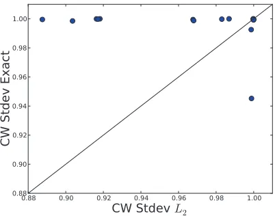
Figure 5: The trained model’s accuracy on the training data for fifteen of the data sets for the exact diagonal andL2 diagonal approximation Stdev methods. Points above the line indicate that the exact algorithm obtained a higher training accuracy than theL2diagonal method. Observe that the exact method almost always obtains a higher training accuracy, and is nearly 100% in every case. Coupled with the results on test data, which are worse for the exact methods, these results indicate that the exact method overfits the training data. These results are typical when comparing the exact algorithms against the diagonal approximations.

is limited. In this setting, we would like an algorithm where individual processors train models on their easily accessible data, and then they combine their models. While this often does not perform as well as a single model trained on all of the data, it is a cost-effective way of learning from very large training sets.

One simple approach is to combine many trained models by averaging their weights (McDonald et al., 2010). However, averaging models trained in parallel assumes that each model has an equally accurate estimate of the model weights. This is obviously not the case where different processors saw different portions of the data, made different updates, or saw features that other processors did not. Rather than taking an average over all models, CW provides a confidence value for each weight, allowing for a more intelligent combination of weights from multiple models.

Since each model is a Gaussian distribution over weights, combining multiple trained CW clas-sifiers is equivalent to combining multiple Gaussian distributions. Specifically, we compute the combined model by finding the Gaussian that minimizes the total divergence to the setCof Gaus-sian distributions (individually trained classifiers) for some divergence operatorD:

min

µ,Σ _c

∑

∈C

D((µ,Σ)_||(µ_c,Σc)),

10 50 100

Number of Parallel Classifiers

90 91 92 93 94 95 96 T e st Ac c u ra c y Reuters

10 50 100

Number of Parallel Classifiers

90 91 92 93 94 95 96 T e st Ac c u ra c y Sentiment Average Uniform Weighted PA Variance

Figure 6: Results for Reuters (800k) and Sentiment (1000k) averaged over 4 runs. Horizontal lines show the test accuracy of a model trained on the entire training set. Vertical bars show the performance ofn (10, 50, 100) classifiers trained on disjoint sections of the data as the average performance, uniform combination, or weighted combination.

This minimization leads to the following weighted combination of individual model means:

µ=

_∑

Σ−_c1 !−1

∑

Σ−_c1µ_c Σ−1=

_∑

Σ−_c1.

We evaluate classifier combination by trainingn(10, 50, 100) models by dividing the example stream intondisjoint parts and report the average performance of each of thenclassifiers (average), the combined classifier from taking the average of thensets of weights (L2) and the combination using the KL divergence on the test data across 4 randomized runs.

Average accuracy on the test sets are reported in Figure 6. As stated above, the PA single model achieves higher accuracy for Reuters, possibly because of the low feature to document ratio. However, combining 10 CW classifiers achieves the best performance. For sentiment, combining 10 classifiers beats PA but is not as good as a single CW model. In every case, combining the classifiers improves over each model individually. On sentiment, the KL combination improves over theL2 combination and in Reuters the models are equivalent. For comparison, we show the accuracy on the test data for a single run on the CW Variance KL model on sentiment data Figure 7. When trained on all of the data and distributed across 10 machines, the classifier loses 1% of its performance which, using Figure 7 as a guide, corresponds to using 22% of the training data.

Finally, we computed the actual run time of both PA and CW on the large data sets to compare the speed of each model. While CW is more complex, requiring more computation per example, the actual speed is comparable to PA; in all tests the run time of the two algorithms was indistin-guishable.

8. Related Work

0 200000 400000 600000 800000 1000000

Number of Training Examples

0.91 0.92 0.93 0.94 0.95

Test Accuracy

Figure 7: Results from CW Variance KL run on the large scale Sentiment data (1000k) averaged over 4 runs. Accuracy on test data is measured every 10k training examples to demon-strate the improvement with increases in training data.

Online additive algorithms have a long history, from the perceptron (Rosenblatt, 1958) to more recent methods (Kivinen and Warmuth, 1997; Crammer et al., 2006b). Our update has a more general form, in which the input vectorxi is linearly transformed using the covariance matrix, both

rotating the input and assigning weight specific learning rates.

The second order perceptron (SOP) (Cesa-Bianchi et al., 2005) demonstrated that second-order techniques can improve first-order online methods. Both SOP and CW maintain second-order in-formation. SOP is mistake driven while CW is passive-aggressive. SOP uses the current example in the correlation matrix for prediction while CW updates after prediction. A variant ofstdevsimilar to SOP follows from our derivation if we fix the Lagrange multiplier in (20) to a predefined value

αi =α, omit the square root, and use a gradient-descent optimization step. Fundamentally, CW algorithms have a probabilistic motivation, while the SOP is geometric: replace the ball around an example with a refined ellipsoid. Shivaswamy and Jebara (2007) used a similar motivation in batch learning.

classifiers, maintaining a multinomial distribution over the experts. We assume linear classifiers as experts and maintain a Gaussian distribution over their weight vectors.

With the growth of available data there is an increasing need for algorithms that process train-ing data very efficiently. A similar approach to ours is to train classifiers incrementally (Bordes and Bottou, 2005). The extreme case is to use each example once, without repetitions, as in the multiplicative update method of Carvalho and Cohen (2006).

In Bayesian modeling, we note few approaches that use parameterized distributions over weight vectors. Borrowing concepts from support vector machines, Jaakkola et al. (1999) developed maxi-mum entropy discrimination, which models the generation of examples with one generative model for each class. The model consisted of distributions over the weights and over margin thresholds. They used Bayesian prediction and set the weights using the maximum-entropy principle. In a more recent approach, Minka et al. (2009) proposed using additional virtual vectors to allow more expressive power beyond Gaussian prior and posterior.

Passing the output of a linear model through a logistic function has a long-history in the statis-tical literature, and is extensively covered in many textbooks (e.g., Hastie et al., 2001). Platt (1998) used similar ideas to convert the output of a support vector machine into probabilistic quantities.

Since the conference versions of this work were published, a few algorithms reminiscent of CW were proposed. Duchi et al. (2010) and McMahan and Streeter (2010) proposed to replace the stan-dard Euclidean distance in stochastic gradient decent with general Mahalanobis distance defined by the second order information, captured by the instantaneous second order moment. Crammer et al. (2009a) proposed to replace the hard constraint enforced by the CW algorithm with a relaxed version, formulated using an additional term in the objective function. They call their algorithm AROW for adaptive regularization of weight vectors. Orabona and Crammer (2010) proposed later a framework for online learning, which contains an algorithm close to AROW as a special case, as well as other new algorithms. From a different perspective, Crammer and Lee (2010) proposed a microscopic view for learning, that tracks individual weight-vectors as opposed only to their macro-scopic quantities, such as mean and covariance. Their algorithm has similar update form as CW ((11) and (13)), yet with different rates.

Finally, Shivaswamy and Jebara (2010b,a) proposed to use second order information, or the variance in the batch setting where an iid distribution over the examples is assumed. Their algorithm both maximizes the (average) margin and at the same time minimizes its variance. Note, that they do not maintain a distribution over weight vectors, and the probability space is induced using the distribution over training examples.

9. Conclusion

Acknowledgments

Most of the work was performed while the authors were in the Department of Computer and Infor-mation Science at the University of Pennsylvania. This research was supported in part by the Israeli Science Foundation grant ISF-1567/10. Koby Crammer is a Horev Fellow, supported by the Taub Foundations.

References

Galen Andrew and Jianfeng Gao. Scalable training of l1-regularized log-linear models. InICML ’07: Proceedings Of The 24th International Conference On Machine Learning, pages 33–40, New York, NY, USA, 2007. ACM. ISBN 978-1-59593-793-3. doi: http://doi.acm.org/10.1145/ 1273496.1273501.

Steffen Bickel. ECML-PKDD discovery challenge overview. In The ECML-PKDD Discovery Challenge Workshop, 2006.

John Blitzer, Mark Dredze, and Fernando Pereira. Biographies, Bollywood, boom-boxes and blenders: Domain adaptation for sentiment classification. In Association For Computational Linguistics (ACL), 2007.

Antoine Bordes and L´eon Bottou. The Huller: a simple and efficient online SVM. InEuropean Conference On Machine Learning( ECML ), LNAI 3720, 2005.

Stephen Boyd and Lieven Vandenberghe.Convex Optimization. Cambridge University Press, 2004. Xavier Carreras, Michael Collins, and Terry Koo. Tag, dynamic programming, and the perceptron for efficient, feature-rich parsing. InConference On Natural Language Learning (CONLL), 2008. Vitor R. Carvalho and William W. Cohen. Single-pass online learning: Performance, voting

schemes and online feature selection. InKDD-2006, 2006.

Nicol´o Cesa-Bianchi and Gabor Lugosi. Prediction, learning, and games. Cambridge University Press, 2006.

Nicol´o Cesa-Bianchi, Yoav Freund, David Haussler, David P. Helmbold, Robert E. Schapire, and Manfred K. Warmuth. How to use expert advice.Journal of the ACM, 44(3):427–485, May 1997. Nicol´o Cesa-Bianchi, Alex Conconi, and Claudio Gentile. A second-order perceptron algorithm.

Siam Journal Of Commutation, 34(3):640–668, 2005.

Chih-Chung Chang and Chih-Jen Lin.LIBSVM: a library for support vector machines, 2001. Soft-ware available athttp://www.csie.ntu.edu.tw/˜cjlin/libsvm.