Discriminative Learning Under Covariate Shift
Steffen Bickel [email protected]
Michael Br ¨uckner [email protected]
Tobias Scheffer [email protected]
University of Potsdam, Department of Computer Science August-Bebel-Str. 89
14482 Potsdam, Germany
Editor: Bianca Zadrozny
Abstract
We address classification problems for which the training instances are governed by an input dis-tribution that is allowed to differ arbitrarily from the test disdis-tribution—problems also referred to as classification under covariate shift. We derive a solution that is purely discriminative: neither training nor test distribution are modeled explicitly. The problem of learning under covariate shift can be written as an integrated optimization problem. Instantiating the general optimization prob-lem leads to a kernel logistic regression and an exponential model classifier for covariate shift. The optimization problem is convex under certain conditions; our findings also clarify the relationship to the known kernel mean matching procedure. We report on experiments on problems of spam filtering, text classification, and landmine detection.
Keywords: covariate shift, discriminative learning, transfer learning
1. Introduction
Most machine learning algorithms are constructed under the assumption that the training data is governed by the exact same distribution which the model will later be exposed to. In practice, control over the data generation process is often less perfect. Training data may be obtained under laboratory conditions that cannot be expected after deployment of a system; spam filters may be used by individuals whose distribution of inbound emails diverges from the distribution reflected in public training corpora; image processing systems may be deployed to foreign geographic regions where vegetation and lighting conditions result in a distinct distribution of input patterns.
The case of distinct training and test distributions in a learning problem has been referred to as covariate shift and sample selection bias—albeit the term sample selection bias actually refers to a case in which each training instance is originally drawn from the test distribution, but is then selected into the training sample with some probability, or discarded otherwise.
The covariate shift model and the missing at random case in the sample selection bias model allow for differences between the training and test distribution of instances; the conditional distri-bution of the class variable given the instance is constant over training and test set.
In the covariate shift problem setting, a training sample is available in matrix XL with row
vectors x1, . . . ,xm. This training sample is governed by an unknown distribution p(x|λ). Vector y
with elements y1, . . . ,ymare the labels for training examples and are drawn according to an unknown
xm+1, . . . ,xm+n. The test data is governed by a different unknown distribution, p(x|θ). Training
and test distribution may differ arbitrarily, but there is only one unknown target conditional class distribution p(y|x).
In discriminative learning tasks such as classification, the classifier’s goal is to produce the correct output given the input. It is widely accepted that this is best performed by discriminative learners that directly maximize a quality measure of the produced output. Model-based optimization criteria such as the joint likelihood of input and output, by contrast, additionally assess how well the classifier models the distribution of input values. This amounts to adding a term to the criterion that is irrelevant for the task at hand.
We contribute a discriminative model for learning under different training and test distribu-tions. The model directly characterizes the divergence between training and test distribution, with-out the intermediate—intrinsically model-based—step of estimating training and test distribution. We formulate the search for all model parameters as an integrated optimization problem. This com-plements the predominant procedure of first estimating the bias of the training sample, and then learning the classifier on a weighted version of the training sample. We show that the integrated optimization can be convex, depending on the model type; it is convex for the exponential model. We derive a Newton gradient descent procedure, leading to a kernel logistic regression and an ex-ponential model classifier for covariate shift.
After reviewing models for differing training and test distributions in Section 2, we introduce our integrated model in Section 3. We derive primal and kernelized classifiers for differing training and test distributions in Sections 4 and 5. In Section 6, we analyze the convexity of the integrated optimization problem. Section 7 describes an approximation to the joint optimization problem and Section 8 reveals a new interpretation of kernel mean matching and analyzes the relationship to our model. In Section 9 we discuss different tuning procedures for learning under covariate shift. Section 10 provides empirical results and Section 11 concludes.
The discriminative model for the logistic loss is described in a prior conference publication (Bickel et al., 2007). Our original results showed that the resulting optimization problem is not con-vex. New findings (Section 6) show that the integrated optimization problem can in fact be convex when the loss function is chosen appropriately. Section 7 describes a two-stage approximation that allows to train virtually any type of classifier under covariate shift. The new Section 8 character-izes the relation to kernel mean matching. New experiments include the exponential target model. Section 10 uses an experimental setting that differs from the setting of Bickel et al. (2007) in the parameter tuning process. In some cases, the new setting has improved the performance of baseline methods.
2. Prior Work
If training and test distributions were known, then the loss on the test distribution could be mini-mized by weighting the loss on the training distribution with an instance-specific factor. Proposi-tion 1 (Shimodaira, 2000) illustrates that the scaling factor has to be pp((xx||θ)λ).
Proposition 1 The expected loss with respect toθequals the expected loss with respect toλwith weights pp((xx|θ)
support of p(x|λ):
E(x,y)∼θ[ℓ(f(x),y)] = E(x,y)∼λ
p(x|θ)
p(x|λ)ℓ(f(x),y)
. (1)
After expanding the expected value into its integral R
ℓ(f(x),y)p(x,y|θ)dθ, the joint distribution p(x,y|λ) is decomposed into p(x|λ)p(y|x,λ). Since p(y|x,λ) =p(y|x) = p(y|x,θ) is the global conditional distribution of the class variable given the instance, Proposition 1 follows. All instances
x with positive p(x|θ)are integrated over. Hence, Equation 1 holds as long as each x with positive
p(x|θ)also has a positive p(x|λ); otherwise, the denominator vanishes. This shows that covariate shift can only be compensated for as long as the training distribution covers the entire support of the test distribution. If a test instance had zero density under the training distribution, the test-to-training density ratio which it would need to be scaled with would incur a zero denominator.
Both, p(x|θ) and p(x|λ) are unknown, but p(x|θ) is reflected in XT, as is p(x|λ) in XL. A
straightforward approach to compensating for covariate shift is to first obtain estimates ˆp(x|θ)and ˆ
p(x|λ) from the test and training data, respectively, using kernel density estimation (Shimodaira, 2000; Sugiyama and M¨uller, 2005). In a second step, the estimated density ratio is used to re-sample the training instances, or to train with weighted examples.
This method decouples the problem. First, it estimates training and test distributions. This step is intrinsically model-based and only loosely related to the ultimate goal of accurate classification. In a subsequent step, the classifier is derived given fixed weights. Since the parameters of the final classifier and the parameters that control the weights are not independent, this decomposition into two optimization steps cannot generally find the optimal setting of the joint parameter vector.
A line of work on learning under sample selection bias has meandered from the statistics and econometrics community into machine learning (Heckman, 1979; Zadrozny, 2004). Sample selec-tion bias relies on a model of the data generaselec-tion process. Test instances are drawn under p(x|θ). Training instances are drawn by first sampling x from the test distribution p(x|θ). A selector vari-ableσthen decides whether x is moved into the training set (σ=1) or moved into the rejected set (σ=−1). For instances in the training set (σ=1) a label is drawn from p(y|x), for the instances in the rejected set the labels are unknown. A typical scenario for sample selection bias is credit scoring. The labeled training sample consists of customers who where given a loan in the past and the rejected sample are customers that asked for but where not given a loan. New customers asking for a loan reflect the test distribution.
In the missing at random case, the selector variable is only dependent on x, but not on y; that is, p(σ=1|x,y,θ,λ) =p(σ=1|x,θ,λ). The distribution of the selector variable then maps the test onto the training distribution:
p(x|λ)∝p(x|θ)p(σ=1|x,θ,λ).
Proposition 2 (Zadrozny, 2004; Bickel and Scheffer, 2007) says that minimizing the loss on in-stances weighted by p(σ|x,θ,λ)−1in fact minimizes the expected loss with respect toθ.
Proposition 2 The expected loss with respect toθis proportional to the expected loss with respect toλwith weights p(σ=1|x,θ,λ)−1 for the loss incurred by each x, provided that the support of p(x|θ)is contained in the support of p(x|λ):
E(x,y)∼θ[ℓ(f(x),y)] ∝ E(x,y)∼λ
1
p(σ=1|x,θ,λ)ℓ(f(x),y)
When the model is implemented, p(σ=1|x,θ,λ) is learned by discriminating the training against the rejected examples; in a second step the target model is learned by following Propo-sition 2 and weighting training examples by p(σ|x,θ,λ)−1. No test examples drawn directly from
p(x|θ) are needed to train the model, only labeled selected and unlabeled rejected examples are required. This is in contrast to the covariate shift model that requires samples drawn from the test distribution, but no selection process is assumed and no rejected examples are needed. Covariate shift models can be applied to learning under sample selection bias in the missing at random setting by treating the selected examples as labeled sample and the union of selected (ignoring the labels) and rejected examples as unlabeled sample.
Propensity scores (Rosenbaum and Rubin, 1983; Lunceford and Davidian, 2004) are applied in settings related to sample selection bias; the training data is again assumed to be drawn from the test distribution p(x|θ)followed by a selection process. The difference to the setting of sample selection bias is that the selected and the rejected examples are labeled. Weighting the selected examples by the inverse of the propensity score p(σ=1|x,λ,θ)−1 and weighting the rejected examples by p(σ=−1|x,λ,θ)−1results in two unbiased samples with respect to the test distribution.
Propensity scoring can precede a variety of analysis steps. This can be the training of a target model on re-weighted data or just a statistical analysis of the two re-weighted samples. A typical application for propensity scores is the analysis of the success of a medical treatment. Patients are selected to be given the treatment and some other patients are selected into the control group. If the selector variable is not independent of x (patients may be chosen for an experimental therapy only if they meet specific requirements), the outcome (e.g., ratio of cured patients) of the two groups cannot be compared directly, propensity scores have to be applied.
Maximum entropy density estimation under sample selection bias has been studied by Dudik et al. (2005). Bickel and Scheffer (2007) impose a Dirichlet process prior on several learning prob-lems with related sample selection bias. Elkan (2001) and Japkowicz and Stephen (2002) investigate the case of training data that is only biased with respect to the class ratio, this can be seen as sample selection bias where the selection only depends on y.
Kernel mean matching (Huang et al., 2007) is a two-step method that first finds weights for the training instances such that the first momentum of training and test sets—that is, their mean value— matches in feature space. The subsequent training step uses these weights. Matching the means in feature space is equivalent to matching all moments of the distributions if a universal kernel is used. Huang et al. (2007) derive a quadratic program from Equation 2 that can be solved with standard optimization tools.Φ(·)is a mapping into a feature space and B is a regularization parameter.
minα
m1∑mi=1αiΦ(xi)−1n∑mi=+mn+1Φ(xi) 2
(2)
subject toαi∈[0,B]and 1
m∑ m
i=1αi−1 ≤ε
Cortes et al. (2008) theoretically analyze the error that gets introduced by estimating sample selection bias from data. Their analysis covers the kernel mean matching procedure and a cluster-based estimation technique.
3. Integrated Model
Our goal is to find model parameters w for a probabilistic classification model f(x) =
argmaxyp(y|x; w). The model should correctly predict labels of the test data XTdrawn from p(x|θ).
A regular maximum a posteriori estimation w′ =argmaxwp(y|XL; w)p(w), would only use the
training data(y,XL)governed by p(x|λ). By ignoring the test data, this estimate will not generally result in a model that predicts the missing labels of the test data with a minimum error because the training distribution p(x|λ)is different from the test distribution p(x|θ).
In the following we devise a probabilistic model that accounts for the difference between train-ing and test distribution. Before we describe the model we define a joint data matrix X that is a concatenation of the matrices XLand XT. The model is based on a binary selector variable s: Given
an instance vector x from the joint matrix X of all available instances, selector variable s decides whether x is drawn into the test data XT (s=−1) or into the training data XL(s=1) in which case y is determined. The variable s is governed by the distribution p(s|x; v). Parameter v characterizes the discrepancy between the training and test distribution. Based on the model for s we can now describe the generative process underlying our model:
1. Draw parameter vectors v and w from prior distributions p(v)and p(w);
2. For each row x in matrix X draw binary variable s from distribution p(s|x; v); accordingly, the likelihood of the vector of all selector variables s is p(s|X; v) =∏m+n
i=1 p(si|xi; v);
3. For all selected training examples (all examples xi with si=1) draw vector y of all labels
from p(y|s,X; w,v).
This generative process corresponds to the following factorization of the joint probability of the vector of labels y, vector of selector variables s, and parameter vectors v and w:
p(y,s,w,v|X) = p(y|s,X; w,v)p(s|X; v)p(w)p(v). (3)
3.1 Maximum A Posteriori Parameter Inference
For parameter inference we want to find parameters w that maximize the posterior probability given all available data (Equation 4). The available data are the data matrix X, the label vector y, and the selection vector s, that splits the data matrix into training and test data. Because the parameter
v is unknown and is not needed for the final classifier the best we can do is to integrate it out
(Equation 5).
w∗ = argmaxwp(w|y,s,X) (4)
= argmaxw
Z
p(w,v|y,s,X)dv. (5)
Integrating over v is computationally infeasible. In Equation 6, the integral is therefore approx-imated by the single assignment of values to the parameters which maximizes the posterior—the
maximum a posteriori (MAP) estimator. In our case, the MAP estimator naturally assigns values to
all parameters, w and v.
(wMAP,vMAP) = argmaxw,vp(w,v|y,s,X) (6)
= argmaxw,vp(y,s,w,v|X) (7)
Equation 7 follows from multiplication with a constant p(y,s|X)and from application of the chain rule. Equation 8 applies the factorization from the generative process of Equation 3.
The class-label posterior p(y|x; wMAP)is conditionally independent of vMAPgiven wMAP. However,
wMAP and vMAP are dependent. Assigning a single MAP value to[w,v]instead of integrating over
v is a common approximation. However, sequential maximization of p(s|X; v) over parameters
v followed by maximization of p(y|s,X; w,v) over parameters w with fixed v would amount to an additional degree of approximation and will not generally coincide with the maximum of the product in Equation 8. Such a sequential maximization corresponds to the predominant two-step procedure for learning under covariate shift.
In the next sections we will discuss the likelihood functions p(y|s,X; w,v)and p(s|X; v)and the optimization problem for parameter inference based on maximization of Equation 8.
3.2 Label Likelihood and Discriminative Weighting Factors
In order to define the label likelihood we first derive a discriminative expression for pp((xx|θ)
|λ) which
will no longer include any density on instances. When p(s=−1)>0, which is implied by the test set not being empty, the definition of s allows us to rewrite the test distribution as p(x|θ) =p(x|s=
−1,θ). Since test instances are only dependent on parameter θbut not on parameter λ, equation
p(x|s=−1,θ) = p(x|s=−1,θ,λ) follows. By an analogous argument, p(x|λ) = p(x|s=1,θ,λ)
when p(s=1)>0. This implies Equation 9.
In Equation 10, Bayes’ rule is applied twice; the two terms of p(x|θ,λ)cancel each other out in Equation 11. Since p(s=−1|x,θ,λ) =1−p(s=1|x,θ,λ), Equation 12 follows.
The conditional p(s=1|x,θ,λ)discriminates training (s=1) against test instances (s=−1).
p(x|θ)
p(x|λ) = p(x|s=−1,θ,λ)
1
p(x|s=1,θ,λ) (9)
= p(s=−1|x,θ,λ)p(x|θ,λ) p(s=−1|θ,λ)
p(s=1|θ,λ)
p(s=1|x,θ,λ)p(x|θ,λ) (10)
= p(s=1|θ,λ) p(s=−1|θ,λ)
p(s=−1|x,θ,λ)
p(s=1|x,θ,λ) (11)
= p(s=1|θ,λ) p(s=−1|θ,λ)
1
p(s=1|x,θ,λ)−1
. (12)
The significance of Equation 12 is that it shows how the optimal example weights, the test-to-training ratio pp((xx||λ)θ), can be determined without knowledge of either training or test density. The right hand side of Equation 12 can be evaluated based on a model that discriminates training against test examples and outputs how much more likely an instance is to occur in the test data than it is to occur in the training data. Instead of potentially high-dimensional densities p(x|θ)and p(x|λ), a conditional distribution of the single binary variable s needs to be modeled.
The expression p(s|x,θ,λ) in Equation 12 corresponds to the parametric model p(s|x; v) of Equation 3. With this model we can predict test-to-training density ratios for the training data in XL
according to Equation 12.
Since our goal is discriminative training, the likelihood function p(y|XL; w)(not taking
training-test difference v into account) would be∏ip(yi|xi; w). By using this likelihood p(y|XL; w)instead
distribution. Intuitively, pp((xx||λ)θ)dictates how many times, on average, x should occur in XLif XLwas
governed by the test distributionθ. When the individual conditional likelihood of x is p(y|x; w), then the likelihood of pp((xx|θ)
|λ) occurrences of x is p(y|x; w)
p(x|θ)
p(x|λ). Using a parametric model p(s|x; v),
according to Equation 12 the test-to-training ratio pp((xx||θ)λ)can be expressed as1
p(s=1) p(s=−1)
1
p(s=1|x; v)−1
.
Therefore, we define the likelihood function as2
p(y|s,X; w,v) = m
∏
i=1p(yi|xi; w)
p(s=1) p(s=−1)
1
p(si=1|xi;v)−1
. (13)
As an immediate corollary of Manski and Lerman (1977), the likelihood function of Equation 13 has the property that when the true value v∗is given, its maximizer over w is a consistent estimator of the true parameter w∗that has produced labels for the test data under the test distributionθ. That is, as the sample grows, the maximizer of Equation 13 converges in probability to the true value w∗ of parameter w.
For the statistical analysis of case-control studies, Prentice and Pyke (1979) estimate the ratio of two odds ratios with a discriminative model using a formula similar to Equation 12. This double odds ratio is a statistical measure of the relative risk of an incidence (e.g., lung cancer) given a specific exposure (e.g., cigarette smoking) based on data from a retrospective study.
3.3 Optimization Problem for Integrated Model
The likelihood function p(s|X; v) resolves to p(si = 1|xi; v) for all training instances and p(si=−1|xi; v)for all test instances:
p(s|X; v) = m
∏
i=1p(si=1|xi; v) m+n
∏
i=m+1p(si=−1|xi; v). (14)
Equation 15 summarizes Equations 6 to 8 and Equation 16 inserts the likelihood models (Equa-tions 13 and 14).
p(w,v|y,s,X) ∝ p(y|s,X; w,v)p(s|X; v)p(w)p(v) (15)
= m
∏
i=1p(yi|xi; w)
p(s=1) p(s=−1)
1
p(si=1|xi;v)−1
!
(16)
m
∏
i=1p(si=1|xi; v) m+n
∏
i=m+1p(si=−1|xi; v) !
p(w)p(v).
Using a logistic model for p(s=1|x; v), we notice that Equation 12 can be simplified as in Equation 17.
p(s=1) p(s=−1)
1
1/(1+exp(−vTx))−1
= p(s=1)
p(s=−1)exp(−v
Tx). (17)
1. For a simplified presentation we drop the conditioning in the prior ratio, that is, p(s|θ,λ) =p(s).
2. The variable s in the prior ratio pp((ss==1)
Optimization Problem 1 is derived from Equation 16 in logarithmic form, using linear mod-els vTxiand wTxi and a logistic model for p(s=1|x; v). Negative log-likelihoods are abbreviated
ℓw(yiwTxi) =−log p(yi|xi; w)andℓv(sivTxi) =−log p(si|xi; v), respectively; this notation
empha-sizes the duality between likelihoods and empirical loss functions. The regularization terms corre-spond to Gaussian priors on v and w with variancesσ2vandσ2w.
Optimization Problem 1 Over all w and v, minimize
m
∑
i=1p(s=1)
p(s=−1)exp(−v
Txi)ℓ
w(yiwTxi) + m+n
∑
i=1ℓv(sivTxi) + 1 2σ2
w
wTw+ 1
2σ2
v
vTv.
4. Primal Learning Algorithm
We derive a Newton gradient descent method that directly minimizes Optimization Problem 1 in the attribute space. To this end, we need to derive the gradient and the Hessian of the objective function. The update rule assumes the form of a set of linear equations that have to be solved for the update vector[∆v,∆w]T. It depends on the current parameters[v,w]T, all combinations of training and test data, and resulting coefficients. In order to express the update rule as a single equation in matrix form, we define
X=
XL XT 0
0 0 XL
,
where XLand XT are the matrices of training vectors and test vectors, respectively.
Theorem 3 The update step for the Newton gradient descent minimization of Optimization Prob-lem 1 is[v′,w′]T←[v,w]T+ [∆
v,∆w]Twith
(XΛXT+S) ∆
v ∆w
=−Xg−S
v w
. (18)
The definitions of coefficientsΛ, S, and g—and the proof of the theorem—can be found in
Ap-pendix A.
Given the parameter w, a test instance x is classified as f(x; w) =sign(wTx).
5. Kernelized Learning Algorithm
We derive a kernelized version of the integrated classifier for differing training and test distributions. A transformationΦmaps instances into a target space in which a kernel function k(xi,xj)calculates
the inner productΦ(xi)TΦ(xj). The update rule (Equation 18) thus becomes
(Φ(X)ΛΦ(X)T+S)
∆ v ∆w
= −Φ(X)g−S
v w
. (19)
Φ(X)is defined by
Φ(X) = Φ
(XL) Φ(XT) 0
0 0 Φ(XL)
According to the Representer Theorem, the optimal separator is a linear combination of exam-ples. Parameter vectorsαandβin the dual space weight the influence of all examples:
v w
= Φ(X)
α β
.
Equation 19 can therefore be rewritten as Equation 20. We now multiply Φ(X)T from the
left to both sides and obtain Equation 21. We replace all resulting occurrences of Φ(X)TΦ(X)
by the kernel matrix K and arrive at Equation 22; S is replaced by S′ such thatΦ(X)TSΦ(X) =
Φ(X)TΦ(X)S′, that is, S′i
,i=σ−v2 for i=1, . . . ,m+n and S′m+n+i,m+n+i=σ−w2 for i=1, . . . ,m. Equation 22 is satisfied when Equation 23 is satisfied. Equation 23 is the update rule for the dual Newton gradient descent.
(Φ(X)ΛΦ(X)T+S)Φ(X)
∆α
∆β
= −Φ(X)g−SΦ(X)
α β
, (20)
Φ(X)T(Φ(X)ΛΦ(X)T+S)Φ(X) ∆α
∆β
= −Φ(X)TΦ(X)g−Φ(X)TSΦ(X)
α β
, (21)
(KΛK+KS′) ∆α
∆β
= −Kg−KS′
α β
, (22)
(ΛK+S′) ∆α
∆β
= −g−S′
α β
. (23)
Given the parameters, test instance x is classified by f(x;β) =sign(∑im=1βik(x,xi)).
6. Convexity Analysis and Solving the Optimization Problems
The following theorem specifies sufficient conditions for convexity of Optimization Problem 1. With this theorem we can easily check whether the integrated classifier for covariate shift is convex for specific models of the negative log-likelihood functions. The negative log-likelihood function
ℓwitself and its first and second derivatives are needed. Equations 31 and 32 in Appendix A define shorthand notation which we will use in the following.
Theorem 4 Optimization Problem 1 is convex if the loss functionℓvis convex andℓwis log-convex
and non-negative. The log-convexity condition is equivalent to
ℓwℓ′′w−ℓ′w2≥0. (24)
Proof Looking at Optimization Criterion 1 we immediately see that the regularizers are convex. If ℓvis convex, the second term is convex as well. We therefore only need to analyze the convexity of the term
m
∑
i=1p(s=1)
p(s=−1)exp(−v
Txi)ℓ
w(yiwTxi).
A sum is convex if the single summands are convex. And a sufficient condition for convexity of a function is that it is non-negative and log-convex. The above expression is non-negative asℓwis non-negative. This means we only need to check whether
log p(s=1)
p(s=−1)−v
Txi+logℓ
is convex. The prior ratio is assumed to be constant. The second term is linear and therefore convex and the third term is the log-convexity condition ofℓw. The second derivative of logℓwis
ℓ−w1ℓ′′w+ℓ−w2ℓ′w2,
thus logℓwis convex ifℓwℓ′′w−ℓ′w2is non-negative.
In order to check Optimization Criterion 1 for convexity we need to choose models of the nega-tive log-likelihoodℓvandℓwand derive their first and second derivatives. These derivations are also needed to actually minimize Optimization Criterion 1 with the Newton update steps derived in the last section.
We use a logistic model ℓv(sivTx) =log(1+exp(−sivTx)); the abbreviations of Appendix A can now be expanded:
ℓ′v,isixi j=−
exp(−sivTxi)
1+exp(−sivTxi)
sixi j; ℓ′′v,ixi jxik=
exp(−sivTxi) (1+exp(−sivTxi))2
xi jxik.
For the target classifier, we detail the derivations for logistic and for exponential models ofℓw. For the logistic model the derivatives ofℓware the same as forℓv, only v needs to be replaced by
w and si by yi. For an exponential model withℓw(yiwTx) =exp(−yiwTx) the abbreviations are
expanded as follows:
ℓ′w,iyixi j =−exp(−yiwTxi)yixi j; ℓ′′w,ixi jxik=exp(−yiwTxi)xi jxik.
Using Theorem 4 we can now easily check the convexity of the integrated classifier with logistic model and with exponential model forℓw.
Corollary 5 With a logistic model for ℓw, the condition of Equation 24 is violated and therefore
Optimization Problem 1 with logistic model forℓwmay not convex in general.
Proof Inserting the logistic function into Equation 24 we get the following solution.
ℓw,iℓ′′w,i−ℓ′w2,i =
exp(−yiwTxi) (1+exp(−yiwTx))2
log(1+exp(−yiwTx))−exp(−yiwTxi). (25)
The fraction in Equation 25 is always positive, the difference term is always negative which violates the condition of Equation 24.
Empirically, we find that it is a good choice to select the parameters of a regular, iid logistic regression classifier as starting point for the Newton gradient search.
One can easily show that the condition of Equation 24 is violated whenℓwis chosen as hinge loss or quadratic loss.
Corollary 6 Optimization Problem 1 with exponential model forℓwis convex.
Proof The exponential loss is non-negative and its logarithm is linear and therefore convex.
This means the global optimum of Optimization Problem 1 with exponential model forℓwcan
7. Two-Stage Approximation to Integrated Model
The previous sections describe a complete solution to the learning problem under covariate shift. Optimization Problem 1 is convex for the exponential model; solving it using the efficient proce-dures derived in Sections 4 and 5 produces a globally optimal solution.
For the logistic model, unfortunately, convexity cannot be guaranteed. Furthermore, the regu-larized regression classifier is deeply embedded in Optimization Problem 1. It would not be easy to replace it by a different type of classifier such as, for instance, a decision tree. We will now discuss an approximation to Optimization Problem 1 which solves two consecutive optimization problems. The first optimization problem produces example-specific weights; the second step generates a clas-sifier from the weighted examples. Both optimization problems are convex for exponential, logistic, and hinge loss as well as for many other loss functions. But most significantly, the two-stage ap-proximation is conceptually simple: the second optimization step can be carried out by any learning procedure that is able to scale the loss incurred by each example using prescribed weight factors. Example-specific weights can easily be incorporated into virtually any learning method. Further-more, as a result of the decomposition into two optimization problems parameter tuning becomes much easier because cross-validation can be used (cf. Section 9).
The derivation in Section 3.1 approximates the integral over v by simultaneously selecting a pair of values which maximize the posterior. This leads to the joint MAP hypothesis over v and w. In the resulting optimization problem, v and w are free parameters. At a higher degree of approximation, one may factorize the posterior (Equation 26) and at first approximate the integral over v by the maximum of p(v|y,s,X)(Equations 29 and 30). Subsequently, the posterior over w is maximized given fixed parameters vMAP′ (Equations 27 and 28).
w∗ = argmaxw
Z
p(w,v|y,s,X)dv
= argmaxw
Z
p(w|y,s,X; v)p(v|y,s,X)dv (26)
≈ argmaxwp(w|y,s,X; vMAP′) (27)
= argmaxwp(y|s,X; w,vMAP′)p(w) (28)
with vMAP′ = argmaxvp(v|y,s,X) (29)
= argmaxvp(s|y,X; v)p(v). (30)
This results in two optimization problems. Only parameter v is free in the first stage (Optimization Problem 2). The test-to-training ratio (Equation 17) can be derived from the resulting value of v.
Optimization Problem 2 Over v, minimize m+n
∑
i=1ℓv(sivTxi) +
1 2σ2
v
vTv.
In the second stage (Optimization Problem 3), the target model parameters w are optimized with constant parameters v and constant example weights. The parameters v are the result of Optimiza-tion Problem 2.
Optimization Problem 3 Over w (v is constant), minimize m
∑
i=1p(s=1)
p(s=−1)exp(−v
Txi)ℓ
w(yiwTxi) +
1 2σ2
w
The criterion of Optimization Problem 3 weights the lossℓw(yiwTxi)that each example incurs such that the sample is matched to the test distribution. The last term 2σ12
ww
Tw is the regularizer of the
regression. Optimization Problem 3 can easily be adapted to virtually any type of classification mechanism by inserting the appropriate loss function ℓw(yiwTxi) and regularizer. Operationally,
an arbitrary classification procedure is applied to a sample that is either resampled from the train-ing data accordtrain-ing to sampltrain-ing distribution pp((s=s=−11))exp(−vTxi), or the classifier is applied to the training data with the example-specific loss scaled according to pp(s(s==−11))exp(−vTxi).
8. Relationship to Kernel Mean Matching
Huang et al. (2007) motivate the kernel mean matching algorithm as a procedure that minimizes the distance between the means of unlabeled and weighted labeled data in feature space. If the kernel is universal this is equivalent to minimizing the difference of the distributions. We derive a new interpretation for kernel mean matching that shows its relation to Optimization Problem 2 and the above two-stage approximation.
Using a hinge loss forℓv(si(vTxi+b))in Optimization Problem 2 and an explicit offset
param-eter b we obtain a regular support vector machine. The kernel matrix of this SVM is
K
(LL) K(LT)
KT
(LT) K(T T)
and the target variables are si∈ {−1,1}. An SVM can heuristically be simplified by setting the dual
parametersαi for the unlabeled examples to a fixed value mn. This can be interpreted as a mixture
between an SVM and a Rocchio classifier. Theαicorresponding to the labeled examples (si=1) are
trained with an SVM; settingαiof all unlabeled examples (si=−1) to mn approximates the negative
class (the unlabeled examples) by their centroid in feature space in accordance with the Rocchio classifier (Joachims, 1997).
The SVM optimization criterion with fixedαi=mn for examples with si=−1 is
min 12αT
LK(LL)αL−mnαTLK(LT)1+12 m2
n21K(T T)1−αTL1−nmn
αL
subject toαi∈
0,σ2
v
and∑mi=1αi=∑ni=1mn =m;
vectorαLdenotes all elementsαiwith i=1, . . . ,m. We can drop the constant terms (αTL1 is constant
because of the second constraint) and arrive at Optimization Problem 4.
Optimization Problem 4
min 12αTLK(LL)αL−mnαTLK(LT)1 subject toαi∈
0,σ2
v
andαTL1=m.
αL
This is the dual objective of kernel mean matching. The only difference is that Huang et al. (2007) relax the second constraint up to a small constantε, their constraint is m(1−ε)≤αT
L1≤m(1+ε).
Empirically we find that setting ε to zero has no impact on the performance. The parameterσ2
v corresponds to parameter B in Equation 2.
In order to solve the second stage (Optimization Problem 3), kernel mean matching does not use re-weighting factors pp((ss==−11))exp(−vTxi−b)but directly uses the dualαiparameters as weights.
9. Parameter Tuning
Optimization Problem 1 relies on hyper-parametersσ2vandσ2wthat need to be tuned. For the two-stage approximation of Section 7 and reference methods like kernel mean matching two similar parameters need to be specified. In addition to the regularization parameters kernel parameters need to be tuned for non-linear kernels. Parameter tuning for covariate shift models is much more difficult than for regular prediction models because in the covariate shift setting there is no labeled data available drawn from the test distribution. Parameter tuning by regular cross-validation on the labeled training data is inappropriate because the labeled training data is not governed by the test distribution.
In the following paragraphs we describe different tuning procedures; two procedures require prior knowledge and one does not require prior knowledge on the hyper-parameters. The tuning procedures with prior knowledge can be used for all described models. The one without prior knowledge cannot be used for kernel mean matching and the one-stage model of Optimization Problem 1.
A typical setting with prior knowledge on the hyper-parameters is when the difference between training and test data is introduced by a covariate shift over time and the input distribution shifts constantly over time. The most recent data is the unlabeled test data and the older data has been labeled and is the training data. In this setting the parameters can be tuned by splitting the labeled training data into two consecutive parts. The tuning models are learned on the part with earlier timestamps and the hyper-parametersσ2v andσ2wand kernel parameters are optimized on the part with later timestamps.
Another setting with prior knowledge is when in addition to the pair of training and test set an additional pair of training and fully labeled test set from a different domain with a similar magnitude of covariate shift is available. This additional set can be used to tune the parameters. Due to the similar magnitude of the covariate shift the optimal parameters for the additional domain are assumed to be a good choice for the parameters of the target domain.
For some two-stage models for covariate shift there is no prior knowledge necessary to tune hyper-parameters. Sugiyama et al. (2008) propose to tune the regularizer of the KLIEP model with cross-validation. In this manner the first stage parameterσ2
v(and kernel parameters) of the two-stage model of Section 7 can be tuned as follows. The training and the test data are both split into training and tuning folds and the hold-out likelihood of the tuning folds is optimized with grid search on σ2
v (and kernel parameters). The hold-out likelihood measures the predictive performance of the model p(s|x; v)with respect to predicting the selector variable s of the hold out examples. Once the regularizer of the first stage is tuned, the second stage parameter σ2w(and kernel parameters) can be tuned with cross-validation on weighted training data (Sugiyama and M¨uller, 2005). The data of training folds as well as the data of tuning folds are weighted with the estimated training-to-test ratio.
Kernel mean matching does not provide out-of-sample predictions and it is therefore difficult to tune the regularization parameter B with cross-validation. The one-stage model of Optimization Problem 1 is also difficult to tune with cross-validation because there is a bidirectional influence between the parametersσ2vandσ2w.
10. Empirical Results
We study the benefit of two versions of the integrated classifier for covariate shift and other reference methods on spam filtering, text classification, and landmine detection problems. The first integrated classifier uses a logistic model forℓw(“integrated log model”), the second an exponential model for
ℓw(“integrated exp model”);ℓvis a logistic model in both cases.
The first baseline is a classifier trained under iid assumption with logisticℓw. All other reference methods consist of a two-stage procedure: first, the difference between training and test distribution is estimated, the classifier is trained on weighted data in a second step. The second method is kernel mean matching (Huang et al., 2007); we setε=√m−1/√m as proposed by the authors. In
the third method, separate density estimates for p(x|λ)and p(x|θ)are obtained using kernel density estimation (Shimodaira, 2000), the bandwidth of the kernel is chosen according to the rule-of-thumb of Silverman (1986).
The last two reference methods rely on the two-stage approximation of Optimization Problems 2 and 3 with a logistic regression (“two-stage LR”) and an exponential model classifier (“two-stage exp model”) as their second stages. The example weights are computed according to Equation 17 using a logistic model in the first stage, p(s=1|x; v)is estimated by training a logistic regression that discriminates training from test examples.
The baselines differ in the first stage, the second stage is based on a logistic regression classifier with weighted examples in all cases but the two-stage exponential model baseline. We use a maxi-mum likelihood estimate of mn for pp((ss==−11)). We use tuning procedures that rely on prior knowledge (cf. Section 9). Short descriptions of the respective tuning data can be found below. For all experi-ments we tune the regularization parameters of all methods (and the variance parameter of the RBF kernels for the landmine experiments) by maximizing AUC on the tuning set.
We use the spam filtering data of Bickel et al. (2007); the collection contains nine different inboxes with test emails (5270 to 10964 emails, depending on inbox) and one set of training emails compiled from various different sources. We use a fixed set of 1000 emails as training data. We randomly select between 32 and 2048 emails from one of the original inboxes. We repeat this process 10 times for 2048 test emails and 20 to 640 times for 1024 to 32 test emails. As tuning data we use the labeled emails from an additional inbox different from the test inboxes.
The performance measure is the rate by which the 1−AUC risk is reduced over the iid baseline (Bickel and Scheffer, 2007); it is computed as 1−11−−AUCAUC
iid. We use linear kernels for all methods.
We analyze the rank of the kernel matrix and find that it fulfills the universal kernel requirement of kernel mean matching; this is due to the high-dimensionality of the data.
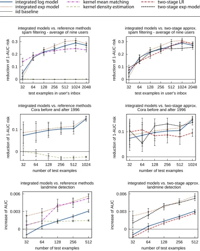
Figure 1 (top row) shows the results for various numbers of unlabeled examples. The left col-umn of Figure 1 compares the integrated classifiers for covariate shift to the kernel mean matching and kernel density estimation baselines. The right column compares the integrated classifiers (Op-timization Problem 1) with the two-stage approximations (Op(Op-timization Problems 2 and 3). The results for a specific number of unlabeled examples are averaged over 10 to 640 random test sam-ples and averaged over all nine inboxes. Averaged over all users and inbox sizes the absolute AUC of the iid classifier is 0.994. Error bars indicate standard errors of the 1−AUC risk.
integrated log model integrated exp model iid baseline
kernel mean matching
kernel density estimation two-stage LRtwo-stage exp model
0 0.1 0.2 0.3
32 64 128 256 512 1024 2048
reduction of 1-AUC risk
test examples in user’s inbox integrated models vs. reference methods
spam filtering - average of nine users
0 0.1 0.2 0.3
32 64 128 256 512 1024 2048
reduction of 1-AUC risk
test examples in user’s inbox integrated models vs. two-stage approx.
spam filtering - average of nine users
0 0.1
32 64 128 256 512 1024
reduction of 1-AUC risk
number of test examples integrated models vs. reference methods
Cora before and after 1996
0 0.1
32 64 128 256 512 1024
reduction of 1-AUC risk
number of test examples integrated models vs. two-stage approx.
Cora before and after 1996
0 0.003 0.006
32 64 128 256 512
increase of AUC
number of test examples integrated models vs. reference methods
landmine detection
0 0.003 0.006
32 64 128 256 512
increase of AUC
number of test examples integrated models vs. two-stage approx.
landmine detection
Figure 1: Average reduction of 1−AUC risk over nine users for spam filtering (top row) and Cora
Machine Learning/Networking classification before and after 1996 (second row) and
convex integrated exponential model performs slightly better than its two-stage approximation; for larger number of test examples (512 to 2048) this difference is statistically significant according to a paired t-test with significance level of 5%. For the logistic model, the two-stage optimization performs similarly well as the integrated version.
We now study text classification using computer science papers from the Cora data set. The task is to discriminate Machine Learning from Networking papers. We select 812 papers written before 1996 from both classes as training examples and 1285 papers written after 1996 as test examples. For parameter tuning we apply an additional time split on the training data; we train on the papers written before 1995 and tune on papers written 1995 (cf. Section 9).
Title and abstract are transformed into tfidf vectors, the number of distinct words is about 40,000. We again use linear kernels (rank analysis verifies the universal kernel property) and aver-age the results over 20 to 640 random test samples for different sizes (1024 for 20 samples to 32 for 640 samples) of test sets. The resulting 1−AUC risk is shown in Figure 1 (second row). The average absolute AUC of the iid classifier is 0.998. The methods based on discriminative density es-timates significantly outperform all other methods. Kernel mean matching is not displayed because its average performance lies far below the iid baseline. The integrated models reduce the 1−AUC risk by 15% for 1024 test examples.
In a third set of experiments we study the problem of detecting landmines using the data set of Xue et al. (2007). The collection contains data of 29 mine fields in different regions. Binary labels (landmine or safe ground) and nine dimensional feature vectors extracted from radar images are provided. There are about 500 examples for each mine field. Each of the fields has a distinct distribution of input patterns, varying from highly foliated to desert areas.
We enumerate all 29×28 pairs of mine fields, using one field as training and the other as test data. For tuning we hold out 4 of the 812 pairs. Results are increases over the iid baseline, averaged over all 29×28−4 combinations. We use RBF kernels with kernel width 0.3 for all methods. The results are displayed in Figure 1 (bottom row). The average absolute AUC of the iid baseline is 0.64 with a standard deviation of 0.07; note, that the error bars are much smaller than the absolute standard deviation because they indicate the standard error of the differences to the iid baseline.
For this problem, the exponential model classifiers and kernel mean matching significantly out-perform all other methods on average. Considering only methods with logistic target model, kernel mean matching is better than all other methods. Integrated logistic regression and two-stage logistic regression are still significantly better than the iid baseline except for 32 and 64 test examples. The integrated classifiers are slightly better than the two-stage variants.
11. Conclusion
We derived a discriminative model for learning under differing training and test distributions. The contribution of each training instance to the optimization problem ideally needs to be weighted with its test-to-training density ratio. We show that this ratio can be expressed—without modeling either training or test density—by a discriminative model that characterizes how much more likely an instance is to occur in the test sample than it is to occur in the training sample.
the joint optimization problem. Theorem 4 specifies the condition for the convexity of Optimiza-tion Problem 1. Checking the condiOptimiza-tion using popular loss funcOptimiza-tions as models of the negative log-likelihoods reveals that Optimization Problem 1 is convex with exponential loss.
We gave a new interpretation for kernel mean matching and show that it is also based on a discriminative model similar to Optimization Problem 2.
Empirically, we found that the integrated and the two-stage models as well as kernel mean matching outperform the iid baseline and the kernel density estimation model in almost all cases. In some cases, the integrated models perform slightly better than their two-stage counterparts. The performance of kernel mean matching depends on the problem; for one out of three problems it did not beat the iid baseline, for the others it yielded comparable results to the integrated models.
The two-stage model is conceptually simpler than the integrated model, and may in some cases have the greatest practical utility. The main advantage compared to the integrated model is that regu-larization parameters can be tuned without prior knowledge by cross-validation. Another advantage of the two-stage model is that in the second stage, after the example-specific weights have been derived, virtually any learning mechanism can be employed to produce the final classifier from the weighted training sample. This comes at the cost of only a marginal loss of performance compared to the integrated model.
Acknowledgments
We gratefully acknowledge support from the German Science Foundation DFG and from STRATO AG. We thank Google for supporting us with a Google Research Award. We also thank the anony-mous reviewers for their helpful comments. We wish to thank Jiayuan Huang, Alex Smola, Arthur Gretton, Karsten Borgward, and Bernhard Sch¨olkopf who provided their implementation of the kernel mean matching algorithm.
Appendix A. Newton Gradient Descent—Proof of Theorem 3
In this Appendix, we derive Newton gradient descent updates for Optimization Problem 1 and thereby prove Theorem 3. We abbreviate
ℓv,i=ℓv(sivTxi); ℓ′v,isixi j=∂
ℓv(sivTxi) ∂vj
; ℓ′′v,ixi jxik=∂ 2ℓ
v(sivTxi)
∂vjvk
; (31)
ℓw,i=ℓw(yiwTxi); ℓ′w,iyixi j=
∂ℓw(yiwTxi)
∂wj
; ℓ′′w,ixi jxik=
∂2ℓ
w(yiwTxi)
∂wjwk
; (32)
ωi=
p(s=1)
p(s=−1)exp(−v
Tx
i)
and denote the objective function of Optimization Problem 1 by
F(v,w) = m
∑
i=1ωiℓw,i+ m+n
∑
i=1ℓv,i+
1 2σ2
w
wTw+ 1
2σ2
v
We compute the gradient with respect to v and w.
∂F(v,w)
∂vj
= − m
∑
i=1ωiℓw,ixi j+ m+n
∑
i=1ℓ′v,isixi j+
1 σ2
v
vj
∂F(v,w)
∂wj =
m
∑
i=1ωiℓ′w,iyixi j+
1 σ2
w
wj.
The Hessian is the matrix of second derivatives.
∂2F(v,w)
∂vj∂vk =
m
∑
i=1ωiℓw,ixi jxik+ m+n
∑
i=1ℓ′′v,ixi jxik+
1 σ2
v δjk
∂2F(v,w)
∂vj∂wk
= − m
∑
i=1ωiℓ′w,iyixi jxik
∂2F(v,w)
∂wj∂wk =
m
∑
i=1ωiℓ′′w,ixi jxik+
1 σ2
w δjk.
We can rewrite the gradient as Xg+S
v w
and the Hessian as XΛXT+S using the following
defini-tions, where d is the dimensionality of XT and XL.
gi=−ωiℓw,i+ℓ′v,i for i=1, . . . ,m;
gm+i=−ℓ′v,m+i for i=1, . . . ,n;
gm+n+i=ωiℓw′ ,iyi for i=1, . . . ,m;
Si,i=σ−v2 for i=1, . . . ,d;
Sd+i,d+i=σ−w2 for i=1, . . . ,d;
Λ= diag
i=1,...,m
ωiℓw,i+ℓ′′v,i
0 − diag
i=1,...,m
(ωiℓ′w,iyi)
0 diag
i=1,...,n ℓ′′
v,m+i
0
− diag
i=1,...,m
(ωiℓ′w,iyi) 0 diag i=1,...,m
(ωiℓ′′w,i) .
The update step for the Newton gradient descent minimization of Optimization Problem 1 is[v′,w′]T←
[v,w]T+ [∆
v,∆w]Twith
(XΛXT+S) ∆
v ∆w
=−Xg−S v w . References
S. Bickel and T. Scheffer. Dirichlet-enhanced spam filtering based on biased samples. In Advances
in Neural Information Processing Systems, 2007.
C. Cortes, M. Mohri, M. Riley, and A. Rostamizadeh. Sample selection bias correction theory. In
Proceedings of the International Conference on Algorithmic Learning Theory, 2008.
M. Dudik, R. Schapire, and S. Phillips. Correcting sample selection bias in maximum entropy density estimation. In Advances in Neural Information Processing Systems, 2005.
C. Elkan. The foundations of cost-sensitive learning. In Proceedings of the International Joint
Conference on Artificial Intellligence, 2001.
J. Heckman. Sample selection bias as a specification error. Econometrica, 47:153–161, 1979.
J. Huang, A. Smola, A. Gretton, K. Borgwardt, and B. Sch¨olkopf. Correcting sample selection bias by unlabeled data. In Advances in Neural Information Processing Systems, 2007.
N. Japkowicz and S. Stephen. The class imbalance problem: A systematic study. Intelligent Data
Analysis, 6:429–449, 2002.
T. Joachims. A probabilistic analysis of the Rocchio algorithm with TFIDF for text categorization. In Proceedings of the 14th International Conference on Machine Learning, 1997.
J. Lunceford and M. Davidian. Stratification and weighting via the propensity score in estimation of causal treatment effects: a comparative study. Statistics in Medicine, 23(19):2937–2960, 2004.
C. Manski and S. Lerman. The estimation of choice probabilities from choice based samples.
Econometrica, 45(8):1977–1988, 1977.
R. Prentice and R. Pyke. Logistic disease incidence models and case-control studies. Biometrika, 66(3):403–411, 1979.
P. Rosenbaum and D. Rubin. The central role of the propensity score in observational studies for causal effects. Biometrika, 70(1):41–55, 1983.
H. Shimodaira. Improving predictive inference under covariate shift by weighting the log-likelihood function. Journal of Statistical Planning and Inference, 90:227–244, 2000.
B. Silverman. Density Estimation for Statistics and Data Analysis. Chapman & Hall, London, 1986.
M. Sugiyama and K.-R. M¨uller. Input-dependent estimation of generalization error under covariate shift. Statistics and Decision, 23(4):249–279, 2005.
M. Sugiyama, S. Nakajima, H. Kashima, P. von B¨unau, and M. Kawanabe. Direct importance estimation with model selection and its application to covariate shift adaptation. In Advances in
Neural Information Processing Systems, 2008.
J. Tsuboi, H. Kashima, S. Hido, S. Bickel, and M. Sugiyama. Direct density ratio estimation for large-scale covariate shift adaptation. In Proceedings of the SIAM International Conference on
Data Mining, 2008.
Y. Xue, X. Liao, L. Carin, and B. Krishnapuram. Multi-task learning for classification with Dirichlet process priors. Journal of Machine Learning Research, 8:35–63, 2007.
B. Zadrozny. Learning and evaluating classifiers under sample selection bias. In Proceedings of the