Multi-Task Learning for Classification with Dirichlet Process Priors
Ya Xue [email protected]
Xuejun Liao [email protected]
Lawrence Carin [email protected]
Department of Electrical and Computer Engineering Duke University
Durham, NC 27708, USA
Balaji Krishnapuram [email protected]
Siemens Medical Solutions USA, Inc. Malvern, PA 19355, USA
Editor: Peter Bartlett
Abstract
Consider the problem of learning logistic-regression models for multiple classification tasks, where the training data set for each task is not drawn from the same statistical distribution. In such a multi-task learning (MTL) scenario, it is necessary to identify groups of similar tasks that should be learned jointly. Relying on a Dirichlet process (DP) based statistical model to learn the extent of similarity between classification tasks, we develop computationally efficient algorithms for two different forms of the MTL problem. First, we consider a symmetric multi-task learning (SMTL) situation in which classifiers for multiple tasks are learned jointly using a variational Bayesian (VB) algorithm. Second, we consider an asymmetric multi-task learning (AMTL) formulation in which the posterior density function from the SMTL model parameters (from previous tasks) is used as a prior for a new task: this approach has the significant advantage of not requiring storage and use of all previous data from prior tasks. The AMTL formulation is solved with a simple Markov Chain Monte Carlo (MCMC) construction. Experimental results on two real life MTL problems indicate that the proposed algorithms: (a) automatically identify subgroups of related tasks whose training data appear to be drawn from similar distributions; and (b) are more accurate than simpler approaches such as single-task learning, pooling of data across all tasks, and simplified approximations to DP.
Keywords: classification, hierarchical Bayesian models, Dirichlet process
1. Introduction
tasks may be highly correlated (dependent on each other), but the strategy of isolating each task and learning the corresponding classifier independently does not exploit the potential information one may acquire from other classification tasks.
The fact that some of the classification tasks are correlated (dependent) implies that what is learned from one task is transferable to another. By learning the classifiers in parallel under a unified representation, the transferability of expertise between tasks is exploited to the benefit of all. This expertise transfer is particularly important when we are provided with only a limited amount of training data for learning each classifier. By exploiting data from related tasks, the training data for each task is strengthened and the generalization of the resulting classifier-estimation algorithm is improved.
1.1 Previous Work on MTL
Multi-task learning has been the focus of much interest in the machine learning community over the last decade. Typical approaches to information transfer among tasks include: sharing hidden nodes in neural networks (Baxter, 1995, 2000; Caruana, 1997); placing a common prior in hierarchical Bayesian models (Yu et al., 2003, 2004, 2005; Zhang et al., 2006); sharing parameters of Gaussian processes (Lawrence and Platt, 2004); learning the optimal distance metric for K-Nearest Neighbors (Thrun and O’Sullivan, 1996); sharing a common structure on the predictor space (Ando and Zhang, 2005); and structured regularization in kernel methods (Evgeniou et al., 2005), among others.
In statistics, the problem of combining information from similar but independent experiments has been studied under the category of meta-analysis (Glass, 1976) for a variety of applications in medicine, psychology and education. Researchers collect data from experiments performed at different sites or times—including information from related experiments published in literature—to obtain an overall evaluation on the significance of an experimental effect. Therefore, meta-analysis is also referred to as quantitative synthesis, or overview. The objective of multi-task learning is different from that of meta analysis. Instead of giving an overall evaluation, our objective is to learn multiple tasks jointly, either to improve the learning performance (i.e., classification accuracy) of each individual task, or to boost the performance of a new task by transferring domain knowledge learned from previously observed tasks. Despite the difference in objectives, many of the techniques employed in the statistical literature on meta-analysis can be applied to multi-task learning as well.
Often, the common prior in a hierarchical Bayesian model is specified in a parametric form with unknown hyper-parameters, for example, a Gaussian distribution with unknown mean and variance. Information is transferred between tasks by learning those hyper-parameters using data from all tasks. However, it is preferable to also learn the functional form of the common prior from the data, instead of being pre-defined. In this paper, we provide such a nonparametric hierarchical Bayesian model for jointly learning multiple logistic regression classifiers. Such nonparametric approaches are desirable because it is often difficult to know what the true distribution should be like, and an inappropriate prior could be misleading. Further, the model parameters of individual tasks may have high complexity, and therefore no appropriate parametric form can be found easily.
In the proposed nonparametric hierarchical Bayesian model, the common prior is drawn from the Dirichlet process (DP). The advantage of applying the DP prior to hierarchical models has been addressed in the statistics literature, see for example Mukhopadhyay and Gelfand (1997), Mallick and Walker (1997) and M ¨uller et al. (2004). Research on the Dirichlet process model goes back to Ferguson (1973), who proved that there is positive (non-zero) probability that some sample function of the DP will be as close as desired to any probability function defined on the same support set. Therefore, the DP is rich enough to model the parameters of individual tasks with arbitrarily high complexity, and flexible enough to fit them well without any assumption about the functional form of the prior distribution.
1.1.2 IDENTIFYING THEEXTENT OFSIMILARITIES BETWEENTASKS INMTL
A common assumption in the previous literature on MTL work is that all tasks are (equally) related to each other, but recently there have been a few investigations concerning the extent of relatedness between tasks. An ideal MTL algorithm should be able to automatically identify similarities be-tween tasks and only allow similar tasks to share data or information. Thrun and O’Sullivan (1996) first presented a task-clustering algorithm with K-Nearest Neighbors. Bakker and Heskes (2003) model the common prior in the hierarchical model as a mixture distribution, but two issues exist in that work: (i) Extra “high-level” task characteristics, other than the features used for learning the model parameters of individual tasks, are needed to decide the relative weights of mixture compo-nents; and (ii) the number of mixtures is a pre-defined parameter. Both these issues are avoided in the models presented here. Based only on the features and class labels, the proposed statistical models automatically identify the similarities between the various tasks and adjust the complexity of the model, that is, the number of task clusters, relying on the implicit nonparametric clustering mechanism of the DP (see Sec. 2).
Before we proceed with the technical details, we clarify two issues about task-similarity. First, we define two classification tasks as similar when the two classification boundaries are close, that is, when the weight vectors of two classifiers are similar. Note that this is different from some previous work such as Caruana (1997) where two tasks are defined to be similar if they use the same features to make their decision.
encourages the fitting of the parameters of individual classifiers to their own data. Therefore, the model parameters learned for any task are the result of the tradeoff between sharing with other tasks and retaining the individuality of the current task. This gives similar tasks the chance to share the same model parameters.
As discussed above, the direct use of DP yields identical parameter estimates to similar tasks. One may more generally wish to give similar (but not identical) parameters to similar tasks. This may be accomplished by adding an additional layer of randomness, that is, modeling the prior of the model parameters as a DP mixture (DPM) (Antoniak, 1974), which is a usual solution to the discrete character of DP. We have compared the models with the DPM prior and the DP prior and found that the former underperforms the latter in all our empirical experiments. We hypothesize that this result is attributable to the increase in model complexity, since the DPM prior introduces one more layer in the hierarchical model than the DP prior. Therefore, in this paper we only present the approach of placing a DP prior on the the model parameters of individual tasks.
1.2 Novel Contributions of this Paper
We develop novel solutions to the following problems: (i) joint learning of multiple classification tasks, which may differ in data statistics due to temporal, geographical or other variations; (ii) effi-cient transfer of the information learned from (i) to a new observed task for the purpose of improving the new task’s learning performance. For notational simplification, problem (i) is referred as SMTL (symmetric multi-task learning) and problem (ii) as AMTL (asymmetric multi-task learning). Our discussion is focused on classification tasks, although the proposed methods can be extended di-rectly to regression problems.
The setting of the SMTL is similar to that used in meta analysis. Most meta-analysis work considers only simple linear models for regression problems. Mukhopadhyay and Gelfand (1997) and Ishwaran (2000) discuss the application of DP priors in the general framework of generalized linear models (GLMs). They use the mixed random effects model to capture heterogeneity in the population studied in an experiment. The fixed effects are modeled with a parametric prior while the random effects are mixed over DP. Our work is closely related to their research, in that the logistic regression model, which we use for classification, is a special case of GLMs. Yet, we modify the model to suit the multi-task setting. First, we group the population by task and add an additional constraint that each group share the same model. Second, we place a DP prior on the whole vector of linear coefficients, including both fixed effects and random effects. The linear coefficients of covariates in the logistic regression model correspond to the classifiers in linear classification problems. For our problem, it is too limiting to consider only the variability in the random effect, that is, the intercept of the classification boundary; the variability in the orientation of the classification boundary should be considered as well.
The AMTL problem addressed here is a natural extension of SMTL. In AMTL the compu-tational burden is relatively small and thus a means of Monte Carlo integration with acceptance-rejection is suggested to make predictions for the new task. We note that Yu et al. (2004) propose a hierarchical Bayesian framework for information filtering, which similarly applies a DP prior on individual user profiles. However, due to limitations of the approximate DP prior employed in Yu et al. (2004), their approach differs from ours in two respects: (i) it cannot be used to improve the classification performance of multiple tasks by learning them in parallel, that is, it is not a solution to the SMTL problem; and (ii) in the AMTL case, their approach conducts an effective information transfer to the new observed task only when the size of the training set is large in previous tasks. These points are clarified further in Section 4.
1.3 Organization of the Paper
The remainder of this paper is organized as follows. Section 2 provides an introduction to the Dirichlet process and its application to data clustering. The SMTL problem is addressed in Section 3, which describes the proposed Bayesian hierarchical framework and presents a variational infer-ence algorithm. Section 4 develops an efficient method of information transfer for the AMTL case and compares it with the method presented by Yu et al. (2004). Experimental results are reported in Section 5, demonstrating the application of the proposed models to a landmine detection and an art image retrieval problem. Section 6 concludes the work and outlines future directions.
2. Dirichlet Process
Assume the model parameters of individual tasks, denoted by w, are drawn from a common prior distribution G. The distribution G itself is sampled from a Dirichlet process DP(α,G0), where α is a positive scaling (innovation) parameter and G0 is a base distribution. The mathematical representation of the DP model is
wm|G ∼ G,
G ∼ DP(α,G0).
where m=1, . . . ,M for M tasks.
Integrating out G, the conditional distribution of wm, given observations of the other M−1 w
values w−m={w1,· · ·,wm−1,wm+1,· · ·,wM}, is
p(wm|w−m,α,G0) =
α
M−1+αG0+
1
M−1+α
M
∑
j=1,j6=m
δwj, (1)
whereδwj is the distribution concentrated at the single point wj.
Let w∗k, k=1, . . . ,K, denote the K distinct values among w1, . . . ,wMand n−m,k denote the
num-ber of w’s equal to w∗k, excluding wm. Equation (1) can be rewritten as
p(wm|w−m,α,G0) =
α
M−1+αG0+
1
M−1+α
K
∑
k=1
n−m,kδw∗
k. (2)
population; (ii) the model is flexible, creating new clusters or merging existing clusters to fit the observed data better; (iii) parameterαcontrols the probability of creating a new cluster, with larger αyielding more clusters; (iv) in the limit asα→∞there is a cluster for each w, and since w are drawn from G0, limα→∞G=G0.
The Dirichlet Process has the following important properties:
1. E[G] =G0; the base distribution represents our prior knowledge or expectation concerning G. 2. p(G|w1, . . . ,wM,α,G0) = DP(α+M,Mα+αG0+M+α1
M
∑
j=1
δwj); the posterior of G is still a
Dirichlet process with the updated base distribution Mα+αG0+ 1
M+α
M
∑
j=1
δwj, and a confidence
in this base distribution that is enhanced relative to the confidence in the original base distri-bution G0, reflected in the increased parameterα→α+M.
The lack of an explicit form of G is addressed with the stick-breaking view of the Dirichlet process. Sethuraman (1994) introduces a constructive definition of the Dirichlet process, based upon which Ishwaran and James (2001) characterize the DP priors with a stick-breaking representation
G=
∞
∑
k=1
πkδw∗
k, (3)
where
πk=vk
k−1
∏
i=1
(1−vi).
For each k, vkis drawn from a Beta distribution Be(1,α);1simultaneously another random variable
w∗k is drawn independently from the base distribution G0; w∗k and πk represents the location and
weight of the kth stick.
If vKis set to one instead of being drawn from the beta distribution, it yields a truncated
approx-imation to the Dirichlet process
G=
K
∑
k=1
πkδw∗k.
Ishwaran and James (2001) establish two theorems for selecting an appropriate truncation level, leading to a model virtually indistinguishable from the infinite DP model; the truncated DP model is computationally more efficient in practice.
3. Learning Multiple Classification Tasks Jointly (SMTL)
In this section we propose a Bayesian multi-task learning model for jointly estimating classifiers for several data sets. The model automatically identifies relatedness by task clustering with nonparamet-ric methods. A variational Bayesian (VB) approximation is used to learn the posterior distributions of the model parameters.
3.1 Mathematical Model
Consider M tasks, indexed as 1,· · ·,M. Let the data set of task m be
D
m={(xm,n,ym,n): n=1,· · ·,Nm}, where xm,n∈Rd, ym,n∈ {0,1}, and (xm,n,ym,n) are drawn i.i.d. from the underlying
distribution of task m. For task m the conditional distribution of ym,n given xm,n is modeled via
logistic regression as,
p(ym,n|wm,xm,n) =σ(wTmxm,n)ym,n[1−σ(wTmxm,n)]1−ym,n (4)
whereσ(x) =1+exp1(−x)and wmparameterizes the classifier for task m. The goal is to learn{wm}Mm=1 jointly, sharing information between tasks as appropriate, so that the resulting classifiers can accu-rately predict class labels for new test samples for tasks m=1,· · ·,M.
To complete the hierarchical model, we place a Dirichlet process prior on the parameters wm,
which based on the discussion in Section 2 implies clustering of the tasks. The base distribution G0is specified as a d-dimensional multivariate normal distribution Nd(µ,Σ). We define an indicator
variable cm= [cm,1, . . . ,cm,∞]T, which is an all-zero vector except that the kth entry is equal to one if task m belongs to cluster k, using the infinite set of mixture components (clusters) reflected in (3). The data can be seen as drawn from the following generative model, obtained by employing the stick-breaking view of DP:
SMTL Model. Given the parametersα, µ andΣ,
1. Draw vkfrom the Beta distribution Be(1,α)and independently draw w∗k from the base
distri-bution Nd(µ,Σ), k=1, . . . ,∞.
2. πk=vk
k−1
∏
i=1
(1−vi), k=1, . . . ,∞.
3. Draw the indicators(cm,1, . . . ,cm,∞)from a multinomial distribution M∞(1;π1, . . . ,π∞), m= 1, . . . ,M
4. wm= ∞
∏
k=1
(w∗k)cm,k, or in an equivalent form w
m=
∞
∑
k=1
cm,kw∗k, m=1, . . . ,M.
5. Draw ym,nfrom a Binomial distribution B(1,σ(wTmxm,n)), m=1, . . . ,M, n=1,· · ·,Nm.
We refer to this as symmetric multi-task learning (SMTL) because all tasks are treated symmet-rically; asymmetric multi-task learning (AMTL) is addressed in Section 4.
3.1.1 HYPER-PRIORS
In the SMTL model,α, µ andΣare given parameters. The scaling parameterαoften has a strong impact on the number of clusters, as analyzed in Section 2. To make the algorithm more robust, it is suggested by West et al. (1994) thatα be integrated over a diffuse hyper-prior. This leads to a modified SMTL model:
SMTL-1 Model. Given the parameters µ,Σand hyper-parametersτ10,τ20,
• Drawαfrom a Gamma distribution Ga(τ10,τ20).
Similarly, we are also interested in the effects of integrating µ and Σ, the parameters of the base distribution, over a diffuse prior. For notational simplification, we useΛ, the precision matrix of the base distribution, instead of the covariance matrix Σ, where Λ=Σ−1. We assume Λ is a diagonal matrix with diagonal elementsλ1,· · ·,λd. The conjugate prior for the mean and precision
of a normal distribution is a Normal-Gamma distribution. Hence, the SMTL-1 model can be further modified as
SMTL-2 Model. Given the hyper-parametersτ10,τ20,γ10,γ20andβ0,
• Drawλjfrom a Gamma distribution Ga(γ10,γ20), j=1, ...,d.
• Draw µ from a Normal distribution Nd(0,(β0Λ)−1); draw α from a Gamma distribution
Ga(τ10,τ20).
• Follow Step 1-5 in the SMTL model.
The performance of the SMTL-1 and SMTL-2 models is analyzed in Section 5.1.1.
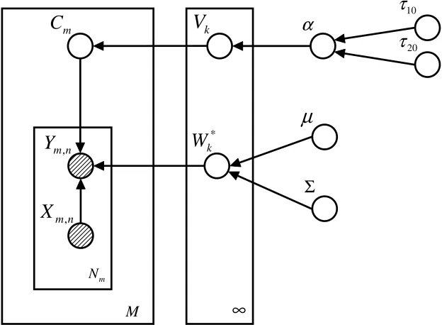
3.1.2 GRAPHICALREPRESENTATION
Figure 1 shows a graphical representation of the SMTL models with the Dirichlet process prior; the two SMTL models differ in the ancestor nodes of w∗k.
In the graph, each node denotes a random variable in the model. The nodes for ym,n and xm,n
are shaded because they are observed data. An arrow indicates dependence between variables, that is, the conditional distribution of a variable given its parents. The number, for example, M, at the lower right corner of a box indicates the nodes in that box have M iid copies.
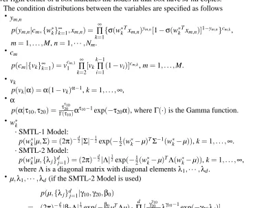
The condition distributions between the variables are specified as follows
·
ym,np(ym,n|cm,{wk∗}∞k=1,xm,n) = ∞
∏
k=1
{σ(w∗
kTxm,n)ym,n[1−σ(w∗kTxm,n)]1−ym,n}cm,k,
m=1, . . . ,M, n=1,· · ·,Nm.
·
cmp(cm|{vk}∞k=1) =v
cm,1
1
∞
∏
k=2
[vk
k−1
∏
i=1
(1−vi)]cm,k, m=1, . . . ,M.
·
vkp(vk|α) =α(1−vk)α−1, k=1, . . . ,∞,
·
αp(α|τ10,τ20) = τ
τ10
20
Γ(τ10)α
τ10−1exp(−τ20α), whereΓ(·)is the Gamma function.
·
w∗k·SMTL-1 Model: p(w∗
k|µ,Σ) = (2π)− d
2|Σ|−12exp(−1
2(w∗k−µ)TΣ−1(w∗k−µ)), k=1, . . . ,∞. ·SMTL-2 Model:
p(w∗k|µ,{λj}dj=1) = (2π)− d
2|Λ| 1
2exp(−1
2(w
∗
k−µ)TΛ(w∗k−µ)), k=1, . . . ,∞,
whereΛis a diagonal matrix with diagonal elementsλ1,· · ·,λd.
·
µ,λ1,· · ·,λd(if the SMTL-2 Model is used)p(µ,{λj}dj=1|γ10,γ20,β0)
= (2π)−d
2|β0Λ| 1
2exp(−β0
2µTΛµ)·
d
∏
j=1
[ γγ2010
Γ(γ10)λ
γ10−1
m
N
∞
M
k
V
α
n m
X
,n m
Y
,m
C
* k
W
10
τ
20
τ
Σ
µ
(a) Graphical representation of the SMTL-1 model.
m
N
∞
M
k
V
α
n m
X
,n m
Y
,m
C
* k
W
10
τ
20
τ
j
λ
µ
d
0 β
10
γ
20
γ
(b) Graphical representation of the SMTL-2 model.
Figure 1: Graphical representation of the SMTL models with the Dirichlet process prior.
andΦ={τ10,τ20,µ,Σ}; for the SMTL-2 model, Z={{cm}Mm=1,{vk}∞k=1,α,{w∗k}∞k=1,µ,{λj}dj=1} andΦ={τ10,τ20,γ10,γ20,β0}.
3.2 Variational Bayesian Inference
In the Bayesian approach, we are interested in p(Z|{
D
m}Mm=1,Φ), the posterior distribution of the latent variables given the observed data and hyper-parameters,p(Z|{
D
m}Mm=1,Φ) =p({
D
m}Mm=1|Z,Φ)p(Z|Φ) p({D
m}Mm=1|Φ),
where p({
D
m}Mm=1|Φ) = Rp({
D
m}Mm=1|Z,Φ)p(Z|Φ)dZ is the marginal distribution, and evaluation of this integration is the principal computational challenge; the integral does not have an analytic form in most cases. The Markov Chain Monte Carlo (MCMC) method is a powerful and popu-lar simulation tool for Bayesian inference. To date most research on applications of the Dirichlet process has been implemented with Gibbs sampling, an MCMC method (Escobar and West, 1995; Ishwaran and James, 2001). However, slow speed and difficult-to-evaluate convergence of the DP Gibbs sampler impede its application in many practical situations.In this work, we employ a computationally efficient approach, mean-field variational Bayesian (VB) inference (Ghahramani and Beal, 2001). The VB method approximates the true posterior p(Z|{
D
m}Mm=1,Φ) by a variational distribution q(Z). It converts computation of posteriors intoan optimization problem of minimizing the Kullback-Leibler (KL) distance between q(Z) and p(Z|{
D
m}Mm=1,Φ), which is equivalent to maximizing a lower bound of log p({D
m}Mm=1|Φ), the log likelihood. To make the optimization problem tractable, it is assumed that the variational distribu-tion q(Z)is sufficiently simple - fully factorized with each factorized component in the exponential family. Under this assumption, an analytic solution of the optimal q(Z)can be obtained by taking functional derivatives; refer to Ghahramani and Beal (2001) and Jordan et al. (1999) for more details about VB.3.2.1 LOCALCONVEXBOUND
One difficulty of applying VB inference to the SMTL models is that the sigmoid function in (4) does not lie within the conjugate-exponential family. We use a variational method based on bounding log convex functions (Jaakkola and Jordan, 1997).
Consider the logistic regression model p(y|w,x) =σ(wTx)y[1−σ(wTx)]1−y. The prior distri-bution of w is assumed to be normal with mean ˜µ0 and variance ˜Σ0. We want to estimate the posterior distribution of w given the data(x,y). This does not have an analytic solution due to the non-exponential property of the logistic regression function. Jaakkola and Jordan (1997) present a method that uses an accurate variational transformation of p(y|w,x)as follows
p(y|w,x)≥σ(ξ)exp((2y−1)w
Tx−ξ
2 +ρ(ξ)(x
TwwTx−ξ2))
,
whereρ(ξ) =
1 2−σ(ξ)
2ξ andξis a variational parameter. The equality holds whenξ=±w
Tx.
The posterior p(w|x,y,˜µ0,Σ0˜ ) remains the normal form with this variational approximation. Given the variational parameter ξ, the mean ˜µ and variance ˜Σ of the normal distribution can be computed as
˜
Σ= (Σ˜−1
0 +2|ρ(ξ)|xx
T)−1
, ˜µ=Σ[˜ Σ˜−1
0 ˜µ0+ (y− 1
Note that we use the top script ˜ to avoid confusion with the usage of µ andΣas the mean and variance of the DP base distribution G0in other sections of this paper.
Since the optimal value ofξdepends on w, an EM algorithm is devised in Jaakkola and Jordan (1997) to optimizeξ. The E step updates ˜µ and ˜Σfollowing (5), given the estimate ofξin the last iteration; the M step computes the optimal value ofξas
ξ2=xT(Σ˜+˜µ˜µT)x
.
This EM algorithm is assured to converge and has been verified to be fast and stable in Jaakkola and Jordan (1997).
The variational method can give us a lower bound of the predictive likelihood as
p(y|x,˜µ0,Σ0˜ )≥exp(logσ(ξ)−ξ
2−ρ(ξ)ξ 2−1
2˜µ
T
0Σ˜−01˜µ0+ 1 2˜µ
TΣ˜−1˜µ+1
2log
|Σ˜|
|Σ0˜ |). (6)
3.2.2 TRUNCATEDVARIATIONALDISTRIBUTION
Another difficulty that must be addressed is the computational complexity of the infinite stick-breaking model. Following Blei and Jordan (2005), we employ a truncated stick-stick-breaking represen-tation for the variational distribution. It is worth noting that in the VB framework, the model is a non-truncated full Dirichlet process while the variational distribution is truncated. Empirical results on truncation level selection are given by Blei and Jordan (2005), but no theoretical criterion has been developed in the VB framework up to now. In all the experiments presented here we set the truncation level equal to the number of tasks. There is no loss of generality with this approach but it is computationally expensive if there are a large number of tasks.
Let K denote the truncation level. In the SMTL-1 model, the factorized variational distribution is specified as
q(Z) = [
M
∏
m=1
qcm(cm)]·[ K
∏
k=1
qvk(vk)]·qα(α)·[( K
∏
k=1
qw∗k(w∗k)],
where
• qcm(cm)is a multinomial distribution,
cm∼MK(1;φm,1, . . . ,φm,K),m=1, . . . ,M. • qvk(vk)is a Beta distribution
vk∼Be(ϕ1,k,ϕ2,k),k=1, . . . ,K−1.
Note qvK(vK) =δ1(vK).
• qα(α)is a Gamma distribution
α∼Ga(τ1,τ2).
• qw∗k(w∗k)is a normal distribution,
Similarly, in the SMTL-2 model, the factorized variational distribution is specified as
q(Z) = [
M
∏
m=1
qcm(cm)]·[ K
∏
k=1
qvk(vk)]·qα(α)·[( K
∏
k=1
qw∗k(w∗k)]·qµ,{λj}dj=1(µ,{λj}
d
j=1).
where qcm(cm), qvk(vk), qα(α)and qw∗k(w ∗
k)are the same as the specifications above.
The distribution qµ,{λj}d
j=1(µ,{λj}
d
j=1)is Normal-Gamma, (µ,{λj}dj=1)∼Nd(η,(βΛ)−1)
d
∏
j=1
Ga(γ1 j,γ2 j). (7)
A coordinate ascent algorithm is developed for the SMTL model by applying the mean-field method (Ghahramani and Beal, 2001). Each factor in the factorized variational distribution andξ, the variational parameter of the sigmoid function, are re-estimated iteratively conditioning on the current estimate of all the others, assuring the lower bound of the log likelihood increases monoton-ically until it converges. The re-estimation equations can be found in the Appendix.
3.3 Prediction for Test Samples
The prediction function for a new test sample xm,?is
p(ym,?=1|cm,{w∗k}Kk=1,xm,?) =
K
∑
k=1
cm,kσ(w∗k T
xm,?). (8)
Integrating (8) over the variational distributions qw∗k(w∗k)and qcm(cm)yields
p(ym,?=1|{{φm,k}Kk=1}Mm=1,{θk}Kk=1,{Γk}Kk=1,xm,?) = ∑K
k=1
φm,k
Rσ(w∗
k
Tx
m,?)Nd(θk,Γk)dw∗k.
(9)
The integral in (9) does not have an analytic form. The variational method described in Section 3.2.1 could give us a lower bound of the integral in the form of (6), if we apply the EM algorithm by taking Nd(θk,Γk)as the prior of w∗k and(xm,?,ym,?=1)as the observation. However, we prefer an accurate estimate of the integral instead of the lower bound of it. In addition, the iterative EM algorithm might be inefficient in some applications that have a strict requirement to the testing speed. Therefore, we use the approximate form of the integral in MacKay (1992)
Z σ(w∗
kTxm,?)Nd(θk,Γk)dw∗k≈σ(
θT
kxm,?
q
1+PI
8xmT,?Γkxm,?
), (10)
where PI is the constant approximately 3.1416 (here PI is used instead ofπto avoid confusion with πused in the stick-breaking representation of the DP).
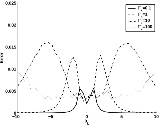
We design a simple experiment to empirically evaluate accuracy of the approximation. Assume xm,? is a 1-dimensional vector. Let the value ofθk be −10,−9.5,· · ·,10 and the value ofΓk be
10−1,100,101and 102. For any combination of the values ofθ
k andΓk, we compare the average
error between the approximation and the true value of the integration over the range of xm,? from
−100 −5 0 5 10 0.005
0.01 0.015 0.02 0.025
θk
Error
Γk=0.1
Γk=1
Γk=10
Γk=100
Figure 2: The error between the approximation and the true value of the integral in (10), averaged over the range of xm,?from−10 to 10 with an interval of 0.5.
method, that is, we randomly draw 104 samples of w∗k from the normal distribution Nd(θk,Γk),
substitute the samples into the logistic functionσ(w∗kTxm,?) and take the average of the function values. The results are plotted in Fig. 2, which shows the approximation is rather accurate.
Substituting (10) into (9) yields the prediction function as
p(ym,?=1|{{φm,k}Kk=1}Mm=1,{θk}Kk=1,{Γk}Kk=1,xm,?)≈
K
∑
k=1
φm,kσ(
θT
kxm,?
q
1+PI
8xTm,?Γkxm,? ).
4. Information Transfer to a New Task (AMTL)
4.1 Prior Learned from Previous Tasks
From (2), we know that the conditional distribution of the classifier wM+1givenα, G0and the other M classifiers is
p(wM+1|w1,· · ·,wM,α,G0) =
α
M+αG0+
1
M+α
K
∑
k=1
nkδw∗
k, (11)
where nk= M
∑
m=1
cm,k is the number of wmwhich are equal to w∗k.
Assume the SMTL-1 model has been applied to M previous tasks and thus the variational distri-butions qcm(cm), qα(α)and qw∗k(w
∗
k)have been optimized. We have Eq[cm,k] =φm,k, Eq[α] =ττ12 and
Eq[w∗k] =θk, where Eqis the expectation with respect to the variational distributions. Substituting
the expectations into (11) yields
p(wM+1|{{φm,k}Kk=1}Mm=1,{θk}Kk=1,τ1,τ2,G0)≈
τ1
τ2
M+τ1
τ2
G0+ 1
M+τ1
τ2
K
∑
k=1
¯nkδθk, (12)
where ¯nk= M
∑
m=1
φm,k. For future convenience, we defineΩ={{{φm,k}Kk=1}Mm=1,{θk}kK=1,τ1,τ2}. Equation (12) represents our belief about the classifier wM+1 before we actually see the data
D
M+1. Therefore, by taking it as a prior for wM+1, information learned from previous tasks canbe transferred to the new task. The posterior of wM+1, after observing the data
D
M+1, is computedaccording to the Bayes Theorem
p(wM+1|
D
M+1,Ω,G0) =p(
D
M+1|wM+1)p(wM+1|Ω,G0) p(D
M+1|Ω,G0), (13)
where
p(
D
M+1|wM+1) = N∏M+1n=1
p(yM+1,n|wM+1,xM+1,n),
= N∏M+1
n=1
σ(wT
M+1xM+1,n)yM+1,n[1−σ(wTM+1xM+1,n)]1−yM+1,n.
(14)
Note in Section 4 we limit the discussion on learning from previous tasks to the SMTL-1 model, for which the parameters of G0are given; the approach developed in this section can be extended to the SMTL-2 model by substituting the expectations on the parameters of G0into (12).
4.2 Sampling Posterior Using Metropolis-Hastings Algorithm
Metropolis-Hastings Algorithm
1. Draw a sample ˙w from (12).
2. Draw a candidate ˆw also from (12).
3. Compute the acceptance probability a(wˆ,w) =˙ min[1,pp((DDM+1|wˆ)
M+1|w˙)].
4. Set the new value of ˙w to ˆw with this probability; otherwise let the new value of ˙w be the same as the old value.
5. Repeat Step 2-4 until the required number of samples, denoted by NSAM, are taken.
This yields an approximation to the posterior in (13)
p(wM+1|
D
M+1,Ω,G0)≈ 1NSAM
NSAM
∑
i=1
δw˙i.
4.3 Prediction Algorithm for Test Samples in New Task
Our goal is to learn wM+1so that the resulting classifier can accurately predict the class label for a new test sample xM+1,?. The prediction function is
p(yM+1,?=1|xM+1,?,Ω,G0) = R
p(yM+1,?=1|xM+1,?,wM+1)p(wM+1|
D
M+1,Ω,G0)dwM+1,≈ 1
NSAM
NSAM
∑
i=1
p(yM+1,?=1|xM+1,?,w˙i),
= 1
NSAM
NSAM
∑
i=1
σ w˙Ti xM+1,?
.
(15)
Hence, the entire learning procedure for a new task is
AMTL-1 Algorithm GivenΩand G0,
1. Compute the parameters in (12) - the prior learned from previous M tasks.
2. Draw samples ˙w1,· · ·,w˙NSAM with the Metropolis-Hastings algorithm.
3. Predict for test samples using (15).
4.4 Comparison with Method of Yu et al. (2004)
Yu et al. (2004) present a hierarchical Bayesian framework for information filtering. Their purpose is to find the right information item for an active user, utilizing both item content information and an accumulated database of item ratings cast by a large set of users. The problem is modeled as a classification problem by labeling the items a user likes “1” and “0” otherwise. The learning situation is similar to our AMTL case, if each user is treated as a task. In Yu’s approach, a Dirichlet process prior is learned from the database
p(wM+1|{Dm}Mm=1,α0,G0) = α0
M+α0G0+
1
M+α0
M
∑
m=1
whereα0 and G0 are pre-defined. They treat ˆwmas the maximum a posteriori (MAP) estimate of
task m. The weightsζmare learned with an Expectation Maximization (EM) algorithm presented in
Yu et al. (2004, Section 3).
From the stick-breaking view of DP, the prior in (16) is an approximation to the standard DP, in that the locations of sticks are fixed, at the classifiers learned from individual models, while the weights are inferred with the EM algorithm. This approximation is inappropriate if the training samples in each previous task are not sufficient, so that each task cannot learn an accurate classifier by only using the corresponding user’s profile. In other words, it is not a good use of the information in previous tasks.
Some other approximations are made in the prediction step of Yu’s approach, although they are relatively trivial compared to the approximation to the DP prior mentioned above. For comparison, we develop the second AMTL algorithm with the approximate DP prior.
AMTL-2 Algorithm Given ˆw1,· · ·,wˆM,α0and G0,
1. Optimize the weightsζmin (16) with the EM algorithm in Yu et al. (2004, Section 3).
2. Substitute (12) with (16), then draw samples ˙w1,· · ·,w˙NSAM with the Metropolis-Hastings
al-gorithm.
3. Predict for test samples using (15).
Empirical comparisons of the two AMTL algorithms are reported in Section 5.1.2.
5. Experiments and Results Analysis
An empirical study of the proposed methods is conducted on two real applications: (i) a landmine detection problem, and (ii) an art image retrieval problem.
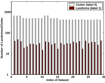
5.1 Landmine Detection
0 5 10 15 20 25 30
1 10 100 1000
Index of Dataset
Number of Landmines/Clutter
Clutter (label 0) Landmine (label 1)
Data from 29 tasks are collected from various landmine fields.2 Each object in a given data set is represented by a 9-dimensional feature vector and the corresponding binary label (1 for landmine and 0 for clutter). The feature vectors are extracted from radar images, concatenating four moment-based features, three correlation-moment-based features, one energy ratio feature and one spatial variance feature. Figure 3 shows the number of landmines/clutter in each data set.
The landmine detection problem is modeled as a binary classification problem. The objective is to learn a classifier from the labeled data, with the goal of providing an accurate prediction for an unlabeled feature vector. We treat classification of each data set as a learning task and evaluate the proposed SMTL and AMTL methods on this landmine detection problem.
Among these 29 data sets, 1-15 correspond to regions that are relatively highly foliated and 16-29 correspond to regions that are bare earth or desert. Thus we expect that there are approximately two clusters of tasks corresponding to two classes of ground surface conditions. We first evaluate the SMTL models using data sets 1-10 and 16-24; next, for the AMTL setting, these data are treated as previous tasks and data sets 11-15 and 25-29 are treated as new observed tasks.
5.1.1 SMTL
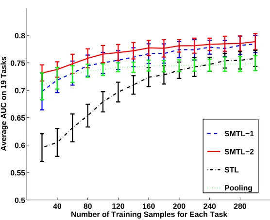
Data sets 1-10 and 16-24 are used for the SMTL experiment, so there are a total of 19 tasks. We ex-amine the performance of four methods on accuracy of label prediction: (i) SMTL-1, (ii) SMTL-2, (iii) the STL method—learn each classifier using the corresponding data set only—with the varia-tional approach to logistic regression models in Section 3.2.1, and (iv) simply pooling the data in all tasks and then learning a single classifier with the variational approach as for (iii).
The performance is measured by average AUC on 19 tasks, where AUC denotes area under the Receiver Operation Characteristic (ROC) curve. A larger AUC value indicates a better classification performance. To have a comprehensive evaluation, we test the algorithms with different sizes of training sets. The number of training samples for every task is set as 20, 40, · · ·, 300. For each task, the training samples are randomly chosen from the corresponding data set and the remaining samples are used for testing. Since the data have severely unbalanced labels, as shown in Fig. 3, we have a special setting that assures there is at least one “1” and one “0” sample in the training set of each task.
Hyper-parameter settings are as follows: (i)τ10=5e−2,τ20=5e−2,γ10=1e−2,γ20=1e−3and β0=1e−2, (ii)τ10=5e−2,τ20=5e−2, µ=0 andΣ=10I, (iii) and (iv) ˜µ0=0 and ˜Σ0=10I. We also tested with other choices of hyper-parameters and found that the algorithms are not sensitive to the hyper-parameter settings as long as the hyper-priors are rather diffuse.
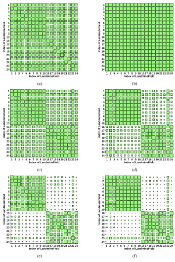
We plot the results of 100 random runs in Fig. 4. The two SMTL methods generally outperform the STL method and simple pooling. To gain insight into how the SMTL method identifies the clustering structure of tasks, we calculate the between-task similarity matrix as follows: at a certain setting of the size of training set (e.g., 20 training samples per task), for each random run, the SMTL algorithm outputs the variational distribution qcm(cm) with the optimized variational parameters
{φm,k}Kk=1, whereφm,k indicates the probability that task m belongs to cluster k, and then we take
km∗ =arg maxkφm,k as the membership of task m. The element at the ith row and jth column in
the between-task similarity matrix records number of occurrences, among 100 random runs, that task i and task j are grouped into the same cluster. Fig. 5 shows the Hinton diagram (Hinton and Sejnowski, 1986) for the between-task similarity matrices corresponding different experiment
40 80 120 160 200 240 280 0.5
0.55 0.6 0.65 0.7 0.75 0.8
Number of Training Samples for Each Task
Average AUC on 19 Tasks
SMTL−1
SMTL−2
STL
Pooling
Figure 4: Average AUC on 19 tasks in the landmine detection problem.
settings: (a)(c)(e) learned by using the SMTL-1 model with 20, 100 and 300 training samples per task; (b)(d)(f) learned by using the SMTL-2 model with 20, 100 and 300 training samples per task. In a Hinton diagram, the size of blocks is proportional to the value of the corresponding matrix elements.
With the help of Fig. 5, we have the following analysis on the behavior of the curves in Fig. 4.
1. When very few training samples are available, for example, 20 per task, the STL method performs poorly. The simple pooling method significantly improves the performance because its effective training size is 18 times larger than that for each individual task. The training samples are so few that although both SMTL methods find that all tasks are similar, they cannot identify the extent of similarity between tasks (see (a) and (b) in Fig. 5). As a result, they perform similar to the simple pooling method. The SMTL-2 performs slightly better due to additional robustness introduced by integrating over the parameters of G0.
2. When there are a few training samples available, for example, 100 per task, the simple pooling method does not improve further as more training samples are pooled together, because it ignores the statistical differences between tasks. Both SMTL methods begin to learn the clustering structure (see (c) and (d) in Fig. 5) and this leads to better performance than the simple pooling. The clustering structure in (d) is more obvious than that in (c), therefore the SMTL-2 method works slightly better than the SMTL-1 method.
1 2 3 4 5 6 7 8 9 10 16 17 18 19 20 21 22 23 24 24 23 22 21 20 19 18 17 16 10 9 8 7 6 5 4 3 2 1
Index of LandmineField
Index of LandmineField
(a)
1 2 3 4 5 6 7 8 9 10 16 17 18 19 20 21 22 23 24 24 23 22 21 20 19 18 17 16 10 9 8 7 6 5 4 3 2 1
Index of LandmineField
Index of LandmineField
(b)
1 2 3 4 5 6 7 8 9 10 16 17 18 19 20 21 22 23 24 24 23 22 21 20 19 18 17 16 10 9 8 7 6 5 4 3 2 1
Index of LandmineField
Index of LandmineField
(c)
1 2 3 4 5 6 7 8 9 10 16 17 18 19 20 21 22 23 24 24 23 22 21 20 19 18 17 16 10 9 8 7 6 5 4 3 2 1
Index of LandmineField
Index of LandmineField
(d)
1 2 3 4 5 6 7 8 9 10 16 17 18 19 20 21 22 23 24 24 23 22 21 20 19 18 17 16 10 9 8 7 6 5 4 3 2 1
Index of LandmineField
Index of LandmineField
(e)
1 2 3 4 5 6 7 8 9 10 16 17 18 19 20 21 22 23 24 24 23 22 21 20 19 18 17 16 10 9 8 7 6 5 4 3 2 1
Index of LandmineField
Index of LandmineField
(f)
in (e) and (f) that the 19 tasks are roughly grouped into two clusters, which agree with the ground truth discussed above.
5.1.2 AMTL
In this experiment, the data sets used in Section 5.1.1 are treated as previous tasks and data sets 11-15 and 25-29 as the new observed tasks. We compare three approaches:
1. AMTL-1: First we apply the SMTL-1 model to those previous tasks and learn the variational parametersΩ, and then run the AMTL-1 algorithm on each new task.
2. AMTL-2: First we apply the variational logistic regression approach in Section 3.2.1 to each previous task and learn the individual classifiers ˆw1, . . . ,wˆM, and then run the AMTL-2
algo-rithm on each new task.
3. STL: Each new task learns by itself.
In the two AMTL methods, the mean and variance of the base distribution G0 are specified as µ=0 andΣ=10I. The parameters τ1 and τ2 in the AMTL-1 model can be estimated from previous tasks, whileα0in the AMTL-2 model is a predefined parameter, which represents a prior belief about the relatedness between the new task and previous tasks. We have two settings: (i) α0=τ1
τ2 =0, which represents a belief that the new task is closely related to previous tasks, and (ii)
α0=τ1
τ2, whereτ1andτ2are estimated from previous tasks.
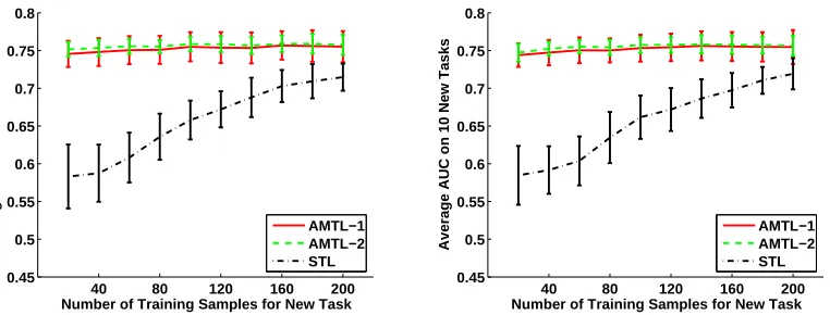
The performance of the three approaches is measured by the average AUC over the 10 new tasks. Experimental results of 100 random runs are shown in Fig. 6. Two factors affecting learning performance are considered: (i) number of training samples per previous task, used for learning the prior of wM+1, and (ii) number of training samples per new task. The first factor is evaluated at 40,
160 and all samples in each previous task used for training, corresponding to (a)(b), (c)(d) and (e)(f) in Fig. 6 respectively. The second factor is evaluated at 20, 40,· · ·, 200 training samples in each new task, plotted along the horizonal axis in each subplot of Fig. 6.
We have the following observations from Fig. 6:
1. In the case α0=τ1
τ2 =0 (see (a)(c)(e)), the prior belief is that the new task is closely related
previous tasks and the purpose of this setting is to focus on the comparison of information transferability of the two AMTL approaches, given the ground truth that the new tasks are quite similar to some of previous tasks. The AMTL-1 approach efficiently transfers informa-tion from previous tasks to the new task. The SMTL method can learn an informative prior for the new task, with only 40 training samples for each previous task (see (a) in Fig. 6). The learning performance is slightly improved by using more training samples for each previous task. The performance has almost no change as the number of training samples in the new task increases, because we use the linear classier and thus the matching classifier can be found with even only a pair of “1” and “0” labeled samples.
40 80 120 160 200 0.45 0.5 0.55 0.6 0.65 0.7 0.75 0.8
Number of Training Samples for New Task
Average AUC on 10 New Tasks
AMTL−1 AMTL−2 STL
(a) α0= ττ12=0; 40 training samples for each previous
task.
40 80 120 160 200
0.45 0.5 0.55 0.6 0.65 0.7 0.75 0.8
Number of Training Samples for New Task
Average AUC on 10 New Tasks
AMTL−1 AMTL−2 STL
(b)α0=ττ12, whereτ1andτ2are estimated from previous
tasks; 40 training samples for each previous task.
40 80 120 160 200
0.45 0.5 0.55 0.6 0.65 0.7 0.75 0.8
Number of Training Samples for New Task
Average AUC on 10 New Tasks
AMTL−1 AMTL−2 STL
(c) α0= ττ12 =0; 160 training samples for each previous
task.
40 80 120 160 200
0.45 0.5 0.55 0.6 0.65 0.7 0.75 0.8
Number of Training Samples for New Task
Average AUC on 10 New Tasks
AMTL−1 AMTL−2 STL
(d)α0=ττ12, whereτ1andτ2are estimated from previous
tasks; 160 training samples for each previous task.
40 80 120 160 200
0.45 0.5 0.55 0.6 0.65 0.7 0.75 0.8
Number of Training Samples for New Task
Average AUC on 10 New Tasks
AMTL−1 AMTL−2 STL
(e) α0= ττ12=0; all samples in previous tasks used for
training.
40 80 120 160 200
0.45 0.5 0.55 0.6 0.65 0.7 0.75 0.8
Number of Training Samples for New Task
Average AUC on 10 New Tasks
AMTL−1 AMTL−2 STL
(f) α0=ττ12, whereτ1andτ2are estimated from previous
tasks; all samples in previous tasks used for training.
of training samples in previous tasks, the AMTL-2 approach works slightly better than the AMTL-1 approach (see (e)), because the former can tell the subtle difference between very similar tasks, while the latter treats them as identical.
2. Next, we recover G0 by using the parametersτ1andτ2estimated from previous tasks in the AMTL-1 model and settingα0= τ1
τ2 in the AMTL-2 model (see (b)(d)(f)). That enables the
new task to discover a new classifier by itself as well as use those learned from previous tasks. Information transferability of the AMTL-2 approach is weak when there are only a few training samples for each previous task, as disussed above. In such a case, the AMTL-2 approach works just as the STL approach because the new task has to learn by itself (see (b)). In contrast, the AMTL-1 approach benefits from previous tasks so that incorporation of G0 has a relatively small effect on its performance.
5.2 Art Image Retrieval
A web survey is built to collect user ratings on 642 paintings from 30 artists.3 A user chooses his rating of an image from “like”,“dislike” or “not sure”. Every user may give ratings only on a subset of all images. In total 203 user ratings are collected.
Our objective is to estimate a user’s preference on unrated images. We model this as a binary classification problem. Each user corresponds to a classification task. The images he rates as “like” are labeled “1”, “dislike” labeled “0” and the images with the rating “not sure” are not included. The content of an image is described by a 275-dimensional (275-D) feature vector concatenating a 256-D correlagram, a 10-D Pyramid wavelet texture and 9-D first and second color moments.
The painting image data differ with the landmine data in two respects. First, the low-level features of image content, for example, color and texture, are weak indicators of human preferences, therefore the content of an image is less helpful than ratings on that image from other users with similar interests. Second, because user preferences are very diverse, the clustering structure of tasks is expected to be more complex than that of the landmine detection tasks.
We use the 68 users who rate more than 100 images for the SMTL experiment. Then we take these as previous tasks and those 50 users who rate between 50 and 100 images are treated as new tasks in the AMTL experiment.
5.2.1 SMTL
In the SMTL experiment, two methods are compared: (i) SMTL-1, and (ii) the single-task learning (STL) method using the variational logistic regression approach in Section 3.2.1. The simple pool-ing method is not feasible because different users may look at the same image and give different ratings. The SMTL-2 model is also excluded, because the feature dimension (275) is high relative to the number of training samples for each task, so that it is hard to get an accurate estimation on the variational distribution ofλj in (7), which is the precision on each feature dimension.
Hyper-parameter settings are as follows: (i) τ10=5e−2, τ20=5e−2, µ=0 and Σ=10I, and (ii) ˜µ0=0 and ˜Σ0=10I. Similar to the landmine experiments, the performance is measured by the average AUC on all tasks and evaluated at 10, 20, 30, 40 or 50 randomly selected training samples for each task. Figure 7 plots the results of 10 random runs.
10 20 30 40 50 0.52
0.53 0.54 0.55 0.56 0.57 0.58 0.59 0.6
Number of Training Samples for Each Task
Average AUC on 68 Tasks
SMTL−1 STL
Figure 7: Average AUC on 68 tasks in the art image retrieval problem.
10 20 30 40 50
20 25 30 35 40
Number of Training Samples for Each Task
Number of Clusters among 68 Tasks
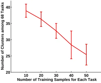
Figure 8: Number of clusters among 68 tasks in the art image retrieval problem.
As mentioned above, the tasks in the art image database are more diverse than those in the landmine data sets. To get a clear view of this, we observe the number of clusters among 68 tasks instead of the between-task similarity matrix. As in Section 5.1.1, we make a hard decision on membership of each task, for each evaluation point and each random run, and then we obtain the statistics of number of clusters among 68 tasks, which is shown in Fig. 8. When the training size is small, the algorithm weakly finds the similarity between tasks and most of the tasks learn by themselves, therefore the SMTL-1 method works similar to the single-task learning. As the number of training samples increases, the clustering structure becomes more clear and information is shared between the users/tasks with similar interests, leading to improvement in learning performance.
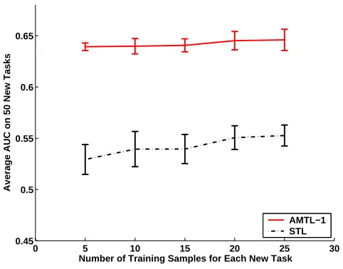
5.2.2 AMTL
0 5 10 15 20 25 30 0.45
0.5 0.55 0.6 0.65
Number of Training Samples for Each New Task
Average AUC on 50 New Tasks
AMTL−1 STL
Figure 9: Average AUC on 50 new tasks in the art image retrieval problem.
algorithm in Section 4.2, NSAM, is set to be 1e3. The results of 10 random runs are shown in Fig. 9.
The curves indicate that the AMTL-1 approach outperforms the STL approach.
6. Conclusions and Future Work
A DP-based multi-task learning algorithm has been applied to the problem of designing logistic-regression classifiers for multiple tasks, for cases in which there is the potential of enhancing individual-task performance via appropriate sharing of inter-task data. Two overarching formu-lations have been considered. In the symmetric multi-task learning (SMTL) formulation all of the task-dependent classifiers are learned jointly. While this is a useful formulation in many cases, it requires one to store all data across previous tasks. In many cases we may undertake a new task and we would like this task to benefit from experience acquired from previous tasks, without having to return to all data observed previously. This has motivated what we have termed an asymmetric multi-task learning (AMTL) formulation. In addition to the overarching SMTL and AMTL for-mulations, we have considered different forms of these algorithms based on how the DP priors are handled.
MTL classification performance has been presented on two data sets: (i) a landmine sensing problem based on measured data, and (ii) an art-preference database. Concerning (i), the MTL formulation yielded a clear indication of how the data from the multiple tasks clustered into related physical phenomena. For this data we know the task-dependent environmental conditions under which the sensing was performed, and the task relatedness reflected in Hinton maps demonstrated close agreement with physical expectations. This provides a powerful confirmation of the utility of the DP formulation for a case in which “truth” is known, yielding confidence for new multi-task data sets for which the DP formulation may be used to infer truth.
formula-tion). For the examples presented here we found the performance of the latter formulation to be slightly better than the former. We also compared the DP MTL formulation to several simpler learning approaches: (i) single-task learning in which no data are shared, (ii) pooling in which all data are shared indiscriminately, and (iii) a simplification to DP developed by Yu et al. (2004). For the data considered, the DP-based MTL formulations developed here outperformed these simpler approaches.
In future research we plan to extend the MTL approach to more-general settings. For exam-ple, in the MTL classifier formulation it is assumed that labeled data are available for each of the tasks. More realistically, labeled data may be available from previous tasks, but the new task un-der investigation may only contain unlabeled data. Based on examining the relationship of the data manifold of the new unlabeled data relative to the manifolds of the previous tasks, it may be possible to ascertain which labeled data, from previous tasks, are relevant for the new unlabeled data under test. In such a heterogeneous MTL setting, involving tasks characterized by labeled and unlabeled data, it may be possible to label the new data under test (from the new task) without requiring any associated labeled data.
In this context one may also consider an active-learning setting, in which labels are acquired selectively from the new task of interest, such that after active learning all tasks have labeled data and the MTL formulations presented here may be applied directly. In this context we note that such an approach was examined in the course of the research presented here, with active learning performed using query by committee (QBC) (McCallum and Nigam, 1998). For the data considered in this paper, we found that as long as at least one label was acquired from each of the two labels (we here considered binary labels), the MTL algorithm performed well. Consequently, while the QBC results were good, even a random acquisition of labels yielded good MTL performance, as long as at least one (randomly acquired) label existed from each of the two labels. This suggests a significant robustness of the MTL formulation, in its ability to use a small amount of labeled data for a given task to still yield good task-dependent classification performance, by appropriately sharing labeled data from other tasks. Nevertheless, this phenomenon is worth further examination, with other data sets, to further examine the utility of active learning as applied to unlabeled data from a new task (relative to simply using random sampling to determine which data to acquire labels on).
Acknowledgments
We would like to acknowledge Kai Yu and Volker Tresp for providing the art image data.
Appendix A. Re-Estimation Equations in Coordinate Ascent Algorithm
• qcm(cm):
sm,k =
Nm
∑
n=1
[−ρ(ξm,n)xTm,n(θkθTk +Γk)xm,n+ (ym,n−12)θTkxm,n
+log(σ(ξm,n))−12ξm,n+ρ(ξm,n)ξ2m,n]
+1(k<K)[Ψ(ϕ1,k)−Ψ(ϕ1,k+ϕ2,k)]
+1(k>1){
k−1
∑
i=1
[Ψ(ϕ2,i)−Ψ(ϕ1,i+ϕ2,i)]}
,
φm,k=
exp(sm,k) K
∑
k=1
exp(sm,k)
,
m=1, . . . ,M,k=1, . . . ,K,
whereΨ(x) =d lndxΓ(x);Γ(x)is the Gamma function; 1(E)is equal to 1 if the logic expression E is true and 0 otherwise.
• qvk(vk):
ϕ1,k=1+ M
∑
m=1
φm,k,
ϕ2,k=
τ1 τ2+
M
∑
m=1
K
∑
i=k+1
φm,i,
k=1, . . . ,K−1.
• q(α):
τ1=τ10+K−1,
τ2=τ20−
K−1
∑
k=1
[Ψ(ϕ2,k)−Ψ(ϕ1,k+ϕ2,k)].
• qw∗k(w∗k):
Γk= [Σ−1+2 M
∑
m=1
φm,k
Nm
∑
n=1
|ρ(ξm,n)|xm,nxTm,n]−1,
θk=Γk[Σ−1µ+ M
∑
m=1
φm,k
Nm
∑
n=1
(ym,n−
1 2)xm,n],
k=1, . . . ,K. (17)
• ξm,n:
ξm,n=
s
K
∑
k=1
φm,kxTm,n(θkθTk +Γk)xm,n,
For the SMTL-2 model, we only need to modify (17) and add an update step for µ andλ1,· · ·,λd
• qw∗k(w∗k):
Γk= [∆+2 M
∑
m=1
φm,k
Nm
∑
n=1
|ρ(ξm,n)|xm,nxTm,n]−1,
θk=Γk[∆η+ M
∑
m=1
φm,k
Nm
∑
n=1
(ym,n−
1 2)xm,n], k=1, . . . ,K,
where∆is a diagonal matrix with diagonal elements γ1,1
γ2,1, . . . ,
γ1,d
γ2,d.
• qµ,{λ
j}dj=1(µ,{λj}
d
j=1):
β=β0+K,
η=
K
∑
k=1
θk
β , γ1,j=γ10+
K 2, γ2,j=γ20+
1 2
K
∑
k=1
(θ2
k,j+Γk,j)−
1 2βη
2
j,
j=1, . . . ,d,
whereθk,j denotes the jth element of the vectorθk (same for ηj), andΓk,j denotes the jth
diagonal element of the matrixΓk.
References
R.K. Ando and T. Zhang. A framework for learning predictive structures from multiple tasks and unlabeled data. Journal of Machine Learning Research, 6:1817C1853, 2005.
C.E. Antoniak. Mixtures of Dirichlet processes with applications to Bayesian nonparametric prob-lems. Annals of Statistics, 2:1152–1174, 1974.
B. Bakker and T. Heskes. Task clustering and gating for Bayesian multitask learning. Journal of Machine Learning Research, 4:83–99, 2003.
J. Baxter. Learning internal representations. In COLT: Proceedings of the Workshop on Computa-tional Learning Theory, 1995.
J. Baxter. A model of inductive bias learning. Journal of Artificial Intelligence Research, 2000.