Dual Averaging Methods for Regularized Stochastic Learning and
Online Optimization
Lin Xiao [email protected]
Microsoft Research 1 Microsoft Way
Redmond, WA 98052, USA
Editor: Sham Kakade
Abstract
We consider regularized stochastic learning and online optimization problems, where the objective function is the sum of two convex terms: one is the loss function of the learning task, and the other is a simple regularization term such asℓ1-norm for promoting sparsity. We develop extensions of Nesterov’s dual averaging method, that can exploit the regularization structure in an online setting. At each iteration of these methods, the learning variables are adjusted by solving a simple mini-mization problem that involves the running average of all past subgradients of the loss function and the whole regularization term, not just its subgradient. In the case ofℓ1-regularization, our method is particularly effective in obtaining sparse solutions. We show that these methods achieve the op-timal convergence rates or regret bounds that are standard in the literature on stochastic and online convex optimization. For stochastic learning problems in which the loss functions have Lipschitz continuous gradients, we also present an accelerated version of the dual averaging method.
Keywords: stochastic learning, online optimization,ℓ1-regularization, structural convex optimiza-tion, dual averaging methods, accelerated gradient methods
1. Introduction
In machine learning, online algorithms operate by repetitively drawing random examples, one at a time, and adjusting the learning variables using simple calculations that are usually based on the single example only. The low computational complexity (per iteration) of online algorithms is often associated with their slow convergence and low accuracy in solving the underlying optimization problems. As argued by Bottou and Bousquet (2008), the combined low complexity and low accu-racy, together with other tradeoffs in statistical learning theory, still make online algorithms favorite choices for solving large-scale learning problems. Nevertheless, traditional online algorithms, such as stochastic gradient descent, have limited capability of exploiting problem structure in solving
regularized learning problems. As a result, their low accuracy often makes it hard to obtain the
desired regularization effects, for example, sparsity underℓ1-regularization.
1.1 Regularized Stochastic Learning
The regularized stochastic learning problems we consider are of the following form:
minimize
w
n
φ(w),Ezf(w,z) +Ψ(w)
o
(1)
where w∈Rnis the optimization variable (often called weights in learning problems), z= (x,y)is
an input-output pair of data drawn from an (unknown) underlying distribution, f(w,z) is the loss
function of using w and x to predict y, and Ψ(w) is a regularization term. We assume Ψ(w) is
a closed convex function (Rockafellar, 1970, Section 7), and its effective domain, domΨ={w∈
Rn|Ψ(w)<+∞}, is closed. We also assume that f(w,z)is convex in w for each z, and it is
subdif-ferentiable (a subgradient always exists) on domΨ. Examples of the loss function f(w,z)include:
• Least-squares: x∈Rn, y∈R, and f(w,(x,y)) = (y−wTx)2.
• Hinge loss: x∈Rn, y∈ {+1,−1}, and f(w,(x,y)) =max{0,1−y(wTx)}.
• Logistic regression: x∈Rn, y∈{+1,−1}, and f(w,(x,y)) =log 1+exp −y(wTx)
.
Examples of the regularization termΨ(w)include:
• ℓ1-regularization: Ψ(w) =λkwk1withλ>0. Withℓ1-regularization, we hope to get a
rela-tively sparse solution, that is, with many entries of the weight vector w being zeroes.
• ℓ2-regularization: Ψ(w) = (σ/2)kwk22, withσ>0. Whenℓ2-regularization is used with the
hinge loss function, we have the standard setup of support vector machines.
• Convex constraints:Ψ(w)is the indicator function of a closed convex set
C
, that is,Ψ(w) =IC(w),
0, if w∈
C
,+∞, otherwise.
We can also consider mixed regularizations such asΨ(w) =λkwk1+ (σ/2)kwk22. These examples
cover a wide range of practical problems in machine learning.
A common approach for solving stochastic learning problems is to approximate the expected
loss functionφ(w)by using a finite set of independent observations z1, . . . ,zT, and solve the
follow-ing problem to minimize the empirical loss:
minimize
w
1
T T
∑
t=1
f(w,zt) +Ψ(w). (2)
By our assumptions, this is a convex optimization problem. Depending on the structure of particular problems, they can be solved efficiently by interior-point methods (e.g., Ferris and Munson, 2003; Koh et al., 2007), quasi-Newton methods (e.g., Andrew and Gao, 2007), or accelerated first-order methods (Nesterov, 2007; Tseng, 2008; Beck and Teboulle, 2009). However, this batch optimization approach may not scale well for very large problems: even with first-order methods, evaluating one single gradient of the objective function in (2) requires going through the whole data set.
In this paper, we consider online algorithms that process samples sequentially as they become
calculate a sequence w1,w2,w3, . . .. Suppose at time t, we have the most up-to-date weight vector wt.
Whenever zt is available, we can evaluate the loss f(wt,zt), and also a subgradient gt ∈∂f(wt,zt)
(here∂f(w,z)denotes the subdifferential of f(w,z)with respect to w). Then we compute wt+1based
on these information.
The most widely used online algorithm is the stochastic gradient descent (SGD) method.
Con-sider the general caseΨ(w) =IC(w) +ψ(w), where IC(w)is a “hard” set constraint andψ(w)is a
“soft” regularization. The SGD method takes the form
wt+1=ΠC wt−αt(gt+ξt)
, (3)
where αt is an appropriate stepsize, ξt is a subgradient of ψat wt, andΠC(·) denotes Euclidean
projection onto the set
C
. The SGD method belongs to the general scheme of stochasticapproxima-tion, which can be traced back to Robbins and Monro (1951) and Kiefer and Wolfowitz (1952). In
general we are also allowed to use all previous information to compute wt+1, and even second-order
derivatives if the loss functions are smooth.
In a stochastic online setting, each weight vector wt is a random variable that depends on
{z1, . . . ,zt−1}, and so is the objective value φ(wt). Assume an optimal solution w⋆ to the
prob-lem (1) exists, and letφ⋆=φ(w⋆). The goal of online algorithms is to generate a sequence{wt}∞t=1
such that
lim
t→∞Eφ(wt) =φ
⋆,
and hopefully with reasonable convergence rate. This is the case for the SGD method (3) if we
choose the stepsize αt =c/√t, where c is a positive constant. The corresponding convergence
rate is O(1/√t), which is indeed best possible for subgradient schemes with a black-box model,
even in the case of deterministic optimization (Nemirovsky and Yudin, 1983). Despite such slow convergence and the associated low accuracy in the solutions (compared with batch optimization using, for example, interior-point methods), the SGD method has been very popular in the machine learning community due to its capability of scaling with very large data sets and good generalization performances observed in practice (e.g., Bottou and LeCun, 2004; Zhang, 2004; Shalev-Shwartz et al., 2007).
Nevertheless, a main drawback of the SGD method is its lack of capability in exploiting prob-lem structure, especially for probprob-lems with explicit regularization. More specifically, the SGD
method (3) treats the soft regularizationψ(w)as a general convex function, and only uses its
sub-gradient in computing the next weight vector. In this case, we can simply lumpψ(w)into f(w,zt)
and treat them as a single loss function. Although in theory the algorithm converges to an optimal solution (in expectation) as t goes to infinity, in practice it is usually stopped far before that. Even in the case of convergence in expectation, we still face (possibly big) variations in the solution due to the stochastic nature of the algorithm. Therefore, the regularization effect we hope to have by solving the problem (1) may be elusive for any particular solution generated by (3) based on finite random samples.
An important example and main motivation for this paper is ℓ1-regularized stochastic
learn-ing, whereΨ(w) =λkwk1. In the case of batch learning, the empirical minimization problem (2)
can be solved to very high precision, for example, by interior-point methods. Therefore simply rounding the weights with very small magnitudes toward zero is usually enough to produce desired
sparsity. As a result,ℓ1-regularization has been very effective in obtaining sparse solutions using
(e.g., Chen et al., 1998). In contrast, the SGD method (3) hardly generates any sparse solution, and its inherent low accuracy makes the simple rounding approach very unreliable. Several prin-cipled soft-thresholding or truncation methods have been developed to address this problem (e.g., Langford et al., 2009; Duchi and Singer, 2009), but the levels of sparsity in their solutions are still unsatisfactory compared with the corresponding batch solutions.
In this paper, we develop regularized dual averaging (RDA) methods that can exploit the struc-ture of (1) more effectively in a stochastic online setting. More specifically, each iteration of the RDA methods takes the form
wt+1=arg min
w
( 1
t t
∑
τ=1
hgτ,wi+Ψ(w) +βt
t h(w)
)
, (4)
where h(w)is an auxiliary strongly convex function, and{βt}t≥1is a nonnegative and
nondecreas-ing input sequence, which determines the convergence properties of the algorithm. Essentially, at each iteration, this method minimizes the sum of three terms: a linear function obtained by
aver-aging all previous subgradients (the dual average), the original regularization functionΨ(w), and
an additional strongly convex regularization term(βt/t)h(w). The RDA method is an extension of
the simple dual averaging scheme of Nesterov (2009), which is equivalent to lettingΨ(w)be the
indicator function of a closed convex set.
For the RDA method to be practically efficient, we assume that the functionsΨ(w)and h(w)are
simple, meaning that we are able to find a closed-form solution for the minimization problem in (4).
Then the computational effort per iteration is only O(n), the same as the SGD method. This
assump-tion indeed holds in many cases. For example, if we letΨ(w) =λkwk1and h(w) = (1/2)kwk22, then
wt+1has an entry-wise closed-from solution. This solution uses a much more aggressive truncation
threshold than previous methods, thus results in significantly improved sparsity (see discussions in Section 5).
In terms of iteration complexity, we show that ifβt=Θ(√t), that is, with order exactly√t, then
the RDA method (4) has the standard convergence rate
Eφ(w¯t)−φ⋆≤O
G
√
t
,
where ¯wt = (1/t)∑tτ=1wτ is the primal average, and G is a uniform upper bound on the norms of
the subgradients gt. If the regularization term Ψ(w) is strongly convex, then settingβt ≤O(lnt)
gives a faster convergence rate O(lnt/t).
For stochastic optimization problems in which the loss functions f(w,z)are all differentiable
and have Lipschitz continuous gradients, we also develop an accelerated version of the RDA method that has the convergence rate
Eφ(wt)−φ⋆≤O(1)
L t2+
Q
√
t
,
where L is the Lipschitz constant of the gradients, and Q2 is an upper bound on the variances of
1.2 Regularized Online Optimization
In online optimization, we use an online algorithm to generate a sequence of decisions wt, one at
a time, for t=1,2,3, . . .. At each time t, a previously unknown cost function ft is revealed, and
we encounter a loss ft(wt). We assume that the cost functions ft are convex for all t ≥1. The
goal of the online algorithm is to ensure that the total cost up to each time t, ∑tτ=1fτ(wτ), is not
much larger than minw∑tτ=1fτ(w), the smallest total cost of any fixed decision w from hindsight.
The difference between these two cost is called the regret of the online algorithm. Applications of online optimization include online prediction of time series and sequential investment (e.g., Cesa-Bianchi and Lugosi, 2006).
In regularized online optimization, we add a convex regularization term Ψ(w) to each cost
function. The regret with respect to any fixed decision w∈domΨis
Rt(w), t
∑
τ=1
fτ(wτ) +Ψ(wτ) −
t
∑
τ=1
fτ(w) +Ψ(w)
. (5)
As in the stochastic setting, the online algorithm can query a subgradient gt ∈∂ft(wt)at each step,
and possibly use all previous information, to compute the next decision wt+1. It turns out that the
simple subgradient method (3) is well suited for online optimization: with a stepsizeαt=Θ(1/√t),
it has a regret Rt(w)≤O(
√
t) for all w∈domΨ (Zinkevich, 2003). This regret bound cannot be
improved in general for convex cost functions. However, if the cost functions are strongly convex,
say with convexity parameterσ, then the same algorithm with stepsizeαt=1/(σt)gives an O(lnt)
regret bound (e.g., Hazan et al., 2006; Bartlett et al., 2008).
Similar to the discussions on regularized stochastic learning, the online subgradient method (3) in general lacks the capability of exploiting the regularization structure. In this paper, we show that the same RDA method (4) can effectively exploit such structure in an online setting, and ensure
the O(√t)regret bound withβt =Θ(√t). For strongly convex regularizations, settingβt =O(lnt)
yields the improved regret bound O(lnt).
Since there is no specifications on the probability distribution of the sequence of functions, nor assumptions like mutual independence, online optimization can be considered as a more general framework than stochastic learning. In this paper, we will first establish regret bounds of the RDA method for solving online optimization problems, then use them to derive convergence rates for solving stochastic learning problems.
1.3 Outline of Contents
The methods we develop apply to more general settings than Rn with Euclidean geometry. In
Section 1.4, we introduce the necessary notations and definitions associated with a general finite-dimensional real vector space.
In Section 2, we present the generic RDA method for solving both the stochastic learning and online optimization problems, and give several concrete examples of the method.
In Section 3, we present the precise regret bounds of the RDA method for solving regularized online optimization problems.
In Section 5, we explain the connections of the RDA method to several related work, and analyze its capability of generating better sparse solutions than other methods.
In Section 6, we give an enhanced version of the ℓ1-RDA method, and present computational
experiments on the MNIST handwritten data set (LeCun et al., 1998). Our experiments show that the RDA method is capable of generate sparse solutions that are comparable to those obtained by batch learning using interior-point methods.
In Section 7, we discuss the RDA methods in the context of structural convex optimization and their connections to incremental subgradient methods. As an extension, we develop an accelerated version of the RDA method for stochastic optimization problems with smooth loss functions. We also discuss in detail the p-norm based RDA methods.
Appendices A-D contain technical proofs of our main results.
1.4 Notations and Generalities
Let
E
be a finite-dimensional real vector space, endowed with a norm k · k. This norm defines asystems of balls:
B
(w,r) ={u∈E
|ku−wk ≤r}. LetE
∗be the vector space of all linear functionson
E
, and leths,widenote the value of s∈E
∗at w∈E
. The dual spaceE
∗ is endowed with thedual normksk∗=maxkwk≤1hs,wi.
A function h :
E
→R∪ {+∞}is called strongly convex with respect to the normk · kif thereexists a constantσ>0 such that
h(αw+ (1−α)u)≤αh(w) + (1−α)h(u)−σ
2α(1−α)kw−uk
2,
∀w,u∈dom h.
The constantσis called the convexity parameter, or the modulus of strong convexity. Let rint
C
denote the relative interior of a convex set
C
(Rockafellar, 1970, Section 6). If h is strongly convexwith modulusσ, then for any w∈dom h and u∈rint(dom h),
h(w)≥h(u) +hs,w−ui+σ
2kw−uk
2,
∀s∈∂h(u).
See, for example, Goebel and Rockafellar (2008) and Juditsky and Nemirovski (2008).
In the special case of the coordinate vector space
E
=Rn, we haveE
=E
∗, and the standardinner product hs,wi=sTw=∑ni=1s(i)w(i), where w(i) denotes the i-th coordinate of w. For the
standard Euclidean norm,kwk=kwk2=
p
hw,wiandksk∗=ksk2. For any w0∈Rn, the function h(w) = (σ/2)kw−w0k22is strongly convex with modulusσ.
For another example, consider the ℓ1-norm kwk=kwk1=∑ni=1|w(i)|and its associated dual
norm kwk∗ = kwk∞ = max1≤i≤n|w(i)|. Let
S
n be the standard simplex in Rn, that is,S
n=w∈Rn+|∑n
i=1w(i)=1 .Then the negative entropy function
h(w) =
n
∑
i=1
w(i)ln w(i)+ln n, (6)
with dom h=
S
n, is strongly convex with respect tok · k1with modulus 1 (see, e.g., Nesterov, 2005,Lemma 3). In this case, the unique minimizer of h is w0= (1/n, . . . ,1/n).
For a closed proper convex function Ψ, we use Arg minwΨ(w) to denote the (convex) set of
minimizing solutions. If a convex function h has a unique minimizer, for example, when h is
Algorithm 1 Regularized dual averaging (RDA) method input:
• an auxiliary function h(w)that is strongly convex on domΨand also satisfies
arg min
w
h(w)∈Arg min
w
Ψ(w). (7)
• a nonnegative and nondecreasing sequence{βt}t≥1.
initialize: set w1=arg minwh(w)and ¯g0=0.
for t=1,2,3, . . . do
1. Given the function ft, compute a subgradient gt∈∂ft(wt).
2. Update the average subgradient:
¯
gt= t−1
t g¯t−1+
1
tgt.
3. Compute the next weight vector:
wt+1=arg min
w
hg¯t,wi+Ψ(w) +
βt t h(w)
. (8)
end for
2. Regularized Dual Averaging Method
In this section, we present the generic RDA method (Algorithm 1) for solving regularized stochastic learning and online optimization problems, and give several concrete examples. To unify notation,
we use ft(w)to denote the cost function at each step t. For stochastic learning problems, we simply
let ft(w) = f(w,zt).
At the input to the RDA method, we need an auxiliary function h that is strongly convex on domΨ. The condition (7) requires that its unique minimizer must also minimize the regularization
functionΨ. This can be done, for example, by first choosing a starting point w0∈Arg minwΨ(w)
and an arbitrary strongly convex function h′(w), then letting
h(w) =h′(w)−h′(w0)− h∇h′(w0),w−w0i.
In other words, h(w)is the Bregman divergence from w0induced by h′(w). If h′is not differentiable,
but subdifferentiable at w0, we can replace∇h′(w0)with a subgradient. The input sequence{βt}t≥1
determines the convergence rate, or regret bound, of the algorithm.
There are three steps in each iteration of the RDA method. Step 1 is to compute a subgradient
of ft at wt, which is standard for all subgradient or gradient based methods. Step 2 is the online
version of computing the average subgradient:
¯
gt =
1
t t
∑
τ=1 gτ.
Step 3 is most interesting and worth further explanation. In particular, the efficiency in
com-puting wt+1determines how useful the method is in practice. For this reason, we assume the
reg-ularization functionsΨ(w)and h(w)are simple. This means the minimization problem in (8) can
be solved with little effort, especially if we are able to find a closed-form solution for wt+1. At first
sight, this assumption seems to be quite restrictive. However, the examples below show that this indeed is the case for many important learning problems in practice.
2.1 RDA Methods with General Convex Regularization
For a general convex regularizationΨ, we can choose any positive sequence{βt}t≥1 that is order
exactly√t, to obtain an O(1/√t)convergence rate for stochastic learning, or an O(√t)regret bound
for online optimization. We will state the formal convergence theorems in Sections 3 and 4. Here,
we give several concrete examples. To be more specific, we choose a parameterγ>0 and use the
sequence
βt =γ
√
t, t=1,2,3, . . . .
• Nesterov’s dual averaging method. LetΨ(w) be the indicator function of a closed convex
set
C
. This recovers the simple dual averaging scheme in Nesterov (2009). If we chooseh(w) = (1/2)kwk22, then the Equation (8) yields
wt+1=ΠC
−
√
t
γ g¯t
=ΠC −
1 γ√t
t
∑
τ=1 gτ
!
. (9)
When
C
={w∈Rn|kwk1≤δ}for some δ>0, we have “hard”ℓ1-regularization. In thiscase, although there is no closed-form solution for wt+1, efficient algorithms for projection
onto theℓ1-ball can be found, for example, in Duchi et al. (2008).
• “Soft”ℓ1-regularization. LetΨ(w) =λkwk1for someλ>0, and h(w) = (1/2)kwk22. In this
case, wt+1has a closed-form solution (see Appendix A for the derivation):
wt(+i)1=
0 if
g¯
(i)
t
≤λ,
− √
t
γ
¯
gt(i)−λsgn ¯gt(i)
otherwise,
i=1, . . . ,n. (10)
Here sgn(·)is the sign or signum function, that is, sgn(ω)equals 1 ifω>0, −1 if ω<0,
and 0 ifω=0. Whenever a component of ¯gt is less thanλin magnitude, the corresponding
component of wt+1is set to zero. Further extensions of theℓ1-RDA method, and associated
computational experiments, are given in Section 6.
• Exponentiated dual averaging method. Let Ψ(w) be the indicator function of the standard
simplex
S
n, and h(w)be the negative entropy function defined in (6). In this case,w(t+i)1= 1
Zt+1
exp
− √
t
γ g¯t(i)
, i=1, . . . ,n,
where Zt+1is a normalization parameter such that∑ni=1w
(i)
t+1=1. This is the dual averaging
We discuss in detail the special case of p-norm RDA method in Section 7.2. Several other
exam-ples, including ℓ∞-norm and a hybrid ℓ1/ℓ2-norm (Berhu) regularization, also admit closed-form
solutions for wt+1. Their solutions are similar in form to those obtained in the context of the FOBOS
algorithm in Duchi and Singer (2009).
2.2 RDA Methods with Strongly Convex Regularization
If the regularization termΨ(w)is strongly convex, we can use any nonnegative and
nondecreas-ing sequence{βt}t≥1that grows no faster than O(lnt), to obtain an O(lnt/t)convergence rate for
stochastic learning, or an O(lnt) regret bound for online optimization. For simplicity, in the
fol-lowing examples, we use the zero sequenceβt =0 for all t≥1. In this case, we do not need the
auxiliary function h(w), and the Equation (8) becomes
wt+1=arg min w
hg¯t,wi+Ψ(w) .
• ℓ2
2-regularization. LetΨ(w) = (σ/2)kwk22for someσ>0. In this case, wt+1=−
1 σg¯t =−
1 σt
t
∑
τ=1 gτ.
• Mixedℓ1/ℓ22-regularization. LetΨ(w) =λkwk1+ (σ/2)kwk22withλ>0 andσ>0. In this
case, we have
w(ti+)1=
0 if|g¯t(i)| ≤λ,
−σ1g¯t(i)−λsgn ¯g
(i)
t
otherwise,
i=1, . . . ,n.
• Kullback-Leibler (KL) divergence regularization. LetΨ(w) =σDKL(wkp), where the given
probability distribution p∈rint
S
n, andDKL(wkp), n
∑
i=1
w(i)ln w
(i)
p(i)
!
.
Here DKL(wkp)is strongly convex with respect tokwk1with modulus 1. In this case,
w(t+i)1= 1
Zt+1 p(i)exp
−σ1g¯t(i)
,
where Zt+1is a normalization parameter such that∑ni=1w
(i)
t+1=1. KL divergence
3. Regret Bounds for Online Optimization
In this section, we give the precise regret bounds of the RDA method for solving regularized online optimization problems. The convergence rates for stochastic learning problems can be established based on these regret bounds, and will be given in the next section. For clarity, we gather here the general assumptions used throughout this paper:
• The regularization termΨ(w)is a closed proper convex function, and domΨis closed. The
symbolσis dedicated to the convexity parameter ofΨ. Without loss of generality, we assume
minwΨ(w) =0.
• For each t≥1, the function ft(w)is convex and subdifferentiable on domΨ.
• The function h(w)is strongly convex on domΨ, and subdifferentiable on rint(domΨ).
With-out loss of generality, assume h(w)has convexity parameter 1 and minwh(w) =0.
We will not repeat these general assumptions when stating our formal results later.
To facilitate regret analysis, we first give a few definitions. For any constant D>0, we define
the set
F
D,w∈domΨh(w)≤D2 , and letΓD= sup w∈FD
inf
g∈∂Ψ(w)kgk∗. (11)
We use the convention infg∈/0kgk∗= +∞, where /0denotes the empty set. As a result, ifΨis not
subdifferentiable everywhere on
F
D, that is, if∂Ψ(w) =/0at some w∈F
D, then we haveΓD= +∞.Note thatΓDis not a Lipschitz-type constant which would be required to be an upper bound on all
the subgradients; instead, we only require that at least one subgradient is bounded in norm byΓDat
every point in the set
F
D.We assume that the sequence of subgradients{gt}t≥1generated by Algorithm 1 is bounded, that
is, there exist a constant G such that
kgtk∗≤G, ∀t≥1. (12)
This is true, for example, if domΨ is compact and each ft has Lipschitz-continuous gradient on
domΨ. We require that the input sequence{βt}t≥1be chosen such that
max{σ,β1}>0, (13)
whereσis the convexity parameter ofΨ(w). For convenience, we letβ0=max{σ,β1}and define
the sequence of regret bounds
∆t,βtD2+ G2
2
t−1
∑
τ=0
1 στ+βτ+
2(β0−β1)G2
(β1+σ)2
, t=1,2,3, . . . , (14)
where D is the constant used in the definition of
F
D. We could always setβ1≥σ, so thatβ0=β1andtherefore the term 2(β0−β1)G2/(β1+σ)2 vanishes in the definition (14). However, whenσ>0,
Theorem 1 Let the sequences{wt}t≥1and{gt}t≥1be generated by Algorithm 1, and assume (12) and (13) hold. Then for any t≥1 and any w∈
F
D, we have:(a) The regret defined in (5) is bounded by∆t, that is,
Rt(w)≤∆t. (15)
(b) The primal variables are bounded as
kwt+1−wk2≤
2 σt+βt
∆t−Rt(w)
. (16)
(c) If w is an interior point, that is,
B
(w,r)⊂F
Dfor some r>0, thenkg¯tk∗≤ΓD−
1
2σr+
1
rt ∆t−Rt(w)
. (17)
In Theorem 1, the bounds on kwt+1−wk2 andkg¯tk∗ depend on the regret Rt(w). More
pre-cisely, they depend on∆t−Rt(w), which is the slack of the regret bound in (15). A smaller slack
is equivalent to a larger regret Rt(w), which means w is a better fixed solution for the online
opti-mization problem (the best one gives the largest regret); correspondingly, the inequality (16) gives
a tighter bound onkwt+1−wk2. In (17), the left-hand sidekg¯tk∗does not depend on any particular
interior point w to compare with, but the right-hand side depends on both Rt(w)and how far w is
from the boundary of
F
D. The tightest bound onkg¯tk∗ can be obtained by taking the infimum ofthe right-hand side over all w∈int
F
D. We further elaborate on part (c) through the following twoexamples:
• Consider the case whenΨ is the indicator function of a closed convex set
C
. In this case,σ=0 and ∂Ψ(w) is the normal cone to
C
at w (Rockafellar, 1970, Section 23). By thedefinition (11), we haveΓD=0 because the zero vector is a subgradient at every w∈
C
, eventhough the normal cones can be unbounded at the boundary of
C
. In this case, ifB
(w,r)⊂F
Dfor some r>0, then (17) simplifies to
kg¯tk∗≤
1
rt ∆t−Rt(w)
.
• Consider the functionΨ(w) =σDKL(w||p)with domΨ=
S
n(assuming p∈rintS
n). In thiscase, domΨ, and hence
F
D, have empty interior. Therefore the bound in part (c) does notapply. In fact, the quantityΓDcan be unbounded anyway. In particular, the subdifferentials
ofΨat the relative boundary of
S
nare all empty. In the relative interior ofS
n, the subgradients(actually gradients) ofΨalways exist, but can become unbounded for points approaching the
relative boundary. Nevertheless, the bounds in parts (a) and (b) still hold.
The proof of Theorem 1 is given in Appendix B. In the rest of this section, we discuss more
3.1 Regret Bound with General Convex Regularization
For a general convex regularization term Ψ, any nonnegative and nondecreasing sequence βt =
Θ(√t) gives an O(√t) regret bound. Here we give detailed analysis for the sequence used in
Section 2.1. More specifically, we choose a constantγ>0 and let
βt =γ
√
t, ∀t≥1. (18)
We have the following corollary of Theorem 1.
Corollary 2 Let the sequences {wt}t≥1 and {gt}t≥1 be generated by Algorithm 1 using{βt}t≥1 defined in (18), and assume (12) holds. Then for any t≥1 and any w∈
F
D:(a) The regret is bounded as
Rt(w)≤
γD2+G
2
γ
√
t.
(b) The primal variables are bounded as
1
2kwt+1−wk
2
≤D2+G
2
γ2 −
1
γ√tRt(w).
(c) If w is an interior point, that is,
B
(w,r)⊂F
Dfor some r>0, thenkg¯tk∗≤ΓD+
γD2+G
2
γ
1
r√t−
1
rtRt(w).
Proof To simplify regret analysis, let γ≥σ. Therefore β0 =β1 =γ. Then ∆t defined in (14)
becomes
∆t=γ
√
tD2+G
2
2γ 1+
t−1
∑
τ=1
1 √τ
!
.
Next using the inequality
t−1
∑
τ=1
1
√τ ≤1+
Z t
1
1
√τdτ=2√t−1,
we get
∆t≤γ
√
tD2+G
2
2γ 1+ 2
√
t−1 =
γD2+G
2
γ
√
t.
Combining the above inequality and the conclusions of Theorem 1 proves the corollary.
The regret bound in Corollary 2 is essentially the same as the online gradient descent method of
Zinkevich (2003), which has the form (3), with the stepsizeαt =1/(γ
√
t). The main advantage of the RDA method is its capability of exploiting the regularization structure, as shown in Section 2. The parameters D and G are not used explicitly in the algorithm. However, we need good estimates
of them for choosing a reasonable value forγ. The bestγthat minimizes the expressionγD2+G2/γ
is
γ⋆= G
which leads to the simplified regret bound
Rt(w)≤2GD
√
t.
If the total number of online iterations T is known in advance, then using a constant stepsize in the classical gradient method (3), say
αt =
1 γ⋆
r 2
T =
D G
r 2
T, ∀t=1, . . . ,T, (19)
gives a slightly improved bound RT(w)≤
√
2GD√T (see, e.g., Nemirovski et al., 2009).
The bound in part (b) does not converge to zero. This result is still interesting because there is no special caution taken in the RDA method, more specifically in (8), to ensure the boundedness
of the sequence wt. In the caseΨ(w) =0, as pointed out by Nesterov (2009), this may even look
surprising since we are minimizing over
E
the sum of a linear function and a regularization term(γ/√t)h(w)that eventually goes to zero.
Part (c) gives a bound on the norm of the dual average. IfΨ(w) is the indicator function of a
closed convex set, thenΓD=0 and part (c) shows that ¯gt actually converges to zero if there exist an
interior w in
F
Dsuch that Rt(w)≥0. However, a properly scaled version of ¯gt,−(√t/γ)g¯t, tracksthe optimal solution; see the examples in Section 2.1.
3.2 Regret Bounds with Strongly Convex Regularization
If the regularization function Ψ(w)is strongly convex, that is, with a convexity parameter σ>0,
then any nonnegative, nondecreasing sequence that satisfiesβt ≤O(lnt)will give an O(lnt)regret
bound. If{βt}t≥1is not the all zero sequence, we can simply choose the auxiliary function h(w) =
(1/σ)Ψ(w). Here are several possibilities:
• Positive constant sequences. For simplicity, letβt=σfor t≥0. In this case,
∆t=σD2+ G2
2σ
t−1
∑
τ=0
1
τ+1≤σD
2+G2
2σ(1+lnt).
• Logarithmic sequences. Letβt=σ(1+lnt)for t≥1. In this case,β0=β1=σand
∆t=σ(1+lnt)D2+ G2
2σ 1+
t−1
∑
τ=1
1 τ+1+lnτ
!
≤
σD2+G
2
2σ
(1+lnt).
• The zero sequence. Letβt=0 for t≥1. In this case,β0=σand
∆t = G2
2σ 1+
t−1
∑
τ=1
1 τ
!
+2G
2
σ ≤
G2
2σ(6+lnt). (20)
WhenΨis strongly convex, we also conclude that, given two different points u and v, the regrets
Rt(u)and Rt(v)cannot be nonnegative simultaneously if t is large enough. To see this, we notice
that if Rt(u)and Rt(v)are nonnegative simultaneously for some t, then part (b) of Theorem 1 implies
kwt+1−uk2≤O
lnt
t
, and kwt+1−vk2≤O
lnt
t
,
which again implies
ku−vk2≤(kwt+1−uk+kwt+1−vk)2≤O
lnt
t
.
Therefore, if the event Rt(u)≥0 and Rt(v)≥0 happens for infinitely many t, we must have u=v.
If u6=v, then eventually at least one of the regrets associated with them will become negative.
However, it is possible to construct sequences of functions ft such that the points with nonnegative
regrets do not converge to a fixed point.
4. Convergence Rates for Stochastic Learning
In this section, we give convergence rates of the RDA method when it is used to solve the regular-ized stochastic learning problem (1), and also the related high probability bounds. These rates and
bounds are established not for the individual wt’s generated by the RDA method, but rather for the
primal average
¯
wt=
1
t t
∑
τ=1
wτ, t≥1.
4.1 Rate of Convergence in Expectation
Theorem 3 Assume there exists an optimal solution w⋆to the problem (1) that satisfies h(w⋆)≤D2 for some D>0, and let φ⋆ =φ(w⋆). Let the sequences {wt}t≥1 and {gt}t≥1 be generated by Algorithm 1, and assume (12) holds. Then for any t≥1, we have:
(a) The expected cost associated with the random variable ¯wt is bounded as
Eφ(w¯t)−φ⋆≤
1
t∆t.
(b) The primal variables are bounded as
Ekwt+1−w⋆k2≤
2 σt+βt
∆t.
(c) If w⋆is an interior point, that is,
B
(w⋆,r)⊂F
Dfor some r>0, thenEkg¯tk∗≤ΓD−
1
2σr+
1
Proof First, we substitute all fτ(·)by f(·,zτ)in the definition of the regret
Rt(w⋆) = t
∑
τ=1
f(wτ,zτ) +Ψ(wτ) −
t
∑
τ=1
f(w⋆,zτ) +Ψ(w⋆) .
Let z[t]denote the collection of i.i.d. random variables(z1, . . . ,zt). All the expectations in Theorem 3
are taken with respect to z[t], that is, the symbol E can be written more explicitly as Ez[t]. We note
that the random variable wτ, where 1≤τ≤t, is a function of(z1, . . . ,zτ−1), and is independent of
(zτ, . . . ,zt). Therefore
Ez[t] f(wτ,zτ)+Ψ(wτ)
=Ez[τ−1] Ezτf(wτ,zτ)+Ψ(wτ)
=Ez[τ−1]φ(wτ) =Ez[t]φ(wτ),
and
Ez[t] f(w⋆,zτ) +Ψ(w⋆)
=Ezτf(w⋆,zτ) +Ψ(w⋆) =φ(w⋆) =φ⋆.
Sinceφ⋆=φ(w⋆) =minwφ(w), we have
Ez[t]Rt(w⋆) = t
∑
τ=1
Ez[t]φ(wτ)−tφ⋆≥0. (21)
By convexity ofφ, we have
φ(w¯t) =φ
1
t t
∑
τ=1 wτ
!
≤ 1t
t
∑
τ=1
φ(wτ)
Taking expectation with respect to z[t]and subtractingφ⋆, we have
Ez[t]φ(w¯t)−φ⋆≤
1
t t
∑
τ=1
Ez[t]φ(w¯τ)−tφ⋆
!
=1
tEz[t]Rt(w
⋆).
Then part (a) follows from that of Theorem 1, which states that Rt(w⋆)≤∆t for all realizations
of z[t]. Similarly, parts (b) and (c) follow from those of Theorem 1 and (21).
Specific convergence rates can be obtained in parallel with the regret bounds discussed in Sec-tions 3.1 and 3.2. We only need to divide every regret bound by t to obtain the corresponding rate
of convergence in expectation. More specifically, using appropriate sequences {βt}t≥1, we have
Eφ(w¯t) converging to φ⋆ with rate O(1/√t) for general convex regularization, and O(lnt/t) for
strongly convex regularization.
The bound in part (b) applies to both the caseσ=0 and the caseσ>0. For the latter, we can
derive a slightly different and more specific bound. WhenΨhas convexity parameterσ>0, so is
the functionφ. Therefore,
φ(wt)≥φ(w⋆) +hs,wt−w⋆i+
σ
2kwt−w
⋆k2,
∀s∈∂φ(w⋆).
Since w⋆is the minimizer ofφ, we must have 0∈∂φ(w⋆)(Rockafellar, 1970, Section 27). Setting
s=0 in the above inequality and rearranging terms, we have
kwt−w⋆k2≤
2
Taking expectation of both sides of the above inequality leads to
Ekwt−w⋆k2≤
2
σ(Eφ(wt)−φ⋆)≤
2
σt∆t, (22)
where in the last step we used part (a) of Theorem 3. This bound directly relate wt to∆t.
Next we take a closer look at the quantity Ekw¯t−w⋆k2. By convexity ofk · k2, we have
Ekw¯t−w⋆k2≤
1
t t
∑
τ=1
Ekwτ−w⋆k2 (23)
Ifσ=0, then it is simply bounded by a constant because each Ekwτ−w⋆k2for 1≤τ≤t is bounded
by a constant. Whenσ>0, the optimal solution w⋆is unique, and we have:
Corollary 4 IfΨis strongly convex with convexity parameterσ>0 andβt=O(lnt), then
Ekw¯t−w⋆k2≤O
(lnt)2
t
.
Proof For the ease of presentation, we consider the caseβt=0 for all t≥1. Substituting the bound
on∆t in (20) into the inequality (22) gives
Ekwt−w⋆k2≤
(6+lnt)G2
tσ2 , ∀t≥1.
Then by (23),
Ekw¯t−w⋆k2≤
1
t t
∑
τ=1
6 τ+
lnτ τ
G2
σ2 ≤
1
t
6(1+lnt) +1
2(lnt)
2
G2
σ2.
In other words, Ekw¯t−w⋆k2 converges to zero with rate O((lnt)2/t). This can be shown for any
βt=O(lnt); see Section 3.2 for other choices ofβt.
As a further note, the conclusions in Theorem 3 still hold if the assumption (12) is weakened to
Ekgtk2∗≤G2, ∀t≥1. (24)
However, we need (12) in order to prove the high probability bounds presented next.
4.2 High Probability Bounds
For stochastic learning problems, in addition to the rates of convergence in expectation, it is often desirable to obtain confidence level bounds for approximate solutions. For this purpose, we start
from part (a) of Theorem 3, which states Eφ(wt)−φ⋆≤(1/t)∆t. By Markov’s inequality, we have
for anyε>0,
Prob φ(w¯t)−φ⋆>ε
≤ ∆εtt. (25)
Theorem 5 Assume there exist constants D and G such that h(w⋆)≤D2, and h(wt)≤D2 and
kgtk∗≤G for all t≥1. Then for anyδ∈(0,1), we have, with probability at least 1−δ,
φ(w¯t)−φ⋆≤
∆t
t +
8GDpln(1/δ)
√
t , ∀t≥1. (26)
Theorem 5 is proved in Appendix C.
From our results in Section 3.1, with the input sequence βt =γ√t for all t≥1, we have∆t =
O(√t)regardless ofσ=0 orσ>0. Therefore,φ(w¯t)−φ⋆=O(1/√t) with high probability. To
simplify further discussion, let γ=G/D, hence ∆t ≤2GD√t (see Section 3.1). In this case, if
δ≤1/e≈0.368, then with probability at least 1−δ,
φ(w¯t)−φ⋆≤
10GDpln(1/δ)
√
t .
Lettingε=10GDpln(1/δ)/√t, then the above bound is equivalent to
Prob(φ(w¯t)−φ⋆>ε)≤exp
− ε
2t
(10GD)2
,
which is much tighter than the one in (25). It follows that for any chosen accuracyεand 0<δ≤1/e,
the sample size
t≥(10GD)
2ln(1/δ)
ε2
guarantees that, with probability at least 1−δ, ¯wt is anε-optimal solution of the original stochastic
optimization problem (1).
WhenΨis strongly convex (σ>0), our results in Section 3.2 show that we can obtain regret
bounds∆t=O(lnt)usingβt=O(lnt). However, the high probability bound in Theorem 5 does not
improve: we still haveφ(w¯t)−φ⋆=O(1/√t), not O(lnt/t). The reason is that the concentration
inequality (Azuma, 1967) used in proving Theorem 5 cannot take advantage of the strong-convexity property. By using a refined concentration inequality due to Freedman (1975), Kakade and Tewari (2009, Theorem 2) showed that for strongly convex stochastic learning problems, with probability
at least 1−4δlnt,
φ(w¯t)−φ⋆≤ Rt(w⋆)
t +4
p
Rt(w⋆) t
r
G2ln(1/δ)
σ +max
16G2
σ ,6B
ln(1/δ)
t .
In our context, the constant B is an upper bound on f(w,z) +Φ(w) for w∈
F
D. Using the regretbound R(w⋆)≤∆t, this gives
φ(w¯t)−φ⋆≤
∆t
t +O
p
∆tln(1/δ)
t +
ln(1/δ)
t
!
.
Here the constants hidden in the O-notation are determined by G,σand D. Plugging in∆t=O(lnt),
we haveφ(w¯t)−φ⋆=O(lnt/t) with high probability. The additional penalty of getting the high
5. Related Work
As we pointed out in Section 2.1, if Ψis the indicator function of a convex set
C
, then the RDAmethod recovers the simple dual averaging scheme in Nesterov (2009). This special case also belongs to a more general primal-dual algorithmic framework developed by Shalev-Shwartz and Singer (2006), which can be expressed equivalently in our notation:
wt+1=arg min
w∈C
1 γ√t
t
∑
τ=1 dτt,w
+h(w)
,
where(d1t, . . . ,dtt)is the set of dual variables that can be chosen at time t. The simple dual averaging scheme (9) is in fact the passive extreme of their framework in which the dual variables are simply chosen as the subgradients and do not change over time, that is,
dτt =gτ, ∀τ≤t, ∀t≥1. (27)
However, with the addition of a general regularization termΨ(w)as in (4), the convergence analysis
and O(√t)regret bound of the RDA method do not follow directly as corollaries of either Nesterov
(2009) or Shalev-Shwartz and Singer (2006). Our analysis in Appendix B extends the framework of Nesterov (2009).
Shalev-Shwartz and Kakade (2009) extended the primal-dual framework of Shalev-Shwartz and
Singer (2006) to strongly convex functions and obtained O(lnt)regret bound. In the context of this
paper, their algorithm takes the form
wt+1=arg min w∈C
1 σt
t
∑
τ=1 dτt,w
+h(w)
,
where σ is the convexity parameter of Ψ, and h(w) = (1/σ)Ψ(w). The passive extreme of this
method, with the dual variables chosen in (27), is equivalent to a special case of the RDA method
withβt=0 for all t≥1.
Other than improving the iteration complexity, the idea of treating the regularization explicitly in each step of a subgradient-based method (instead of lumping it together with the loss function and taking their subgradients) is mainly motivated by practical considerations, such as obtaining
sparse solutions. In the case ofℓ1-regularization, this leads to soft-thresholding type of algorithms,
in both batch learning (e.g., Figueiredo et al., 2007; Wright et al., 2009; Bredies and Lorenz, 2008; Beck and Teboulle, 2009) and the online setting (e.g., Langford et al., 2009; Duchi and Singer, 2009; Shalev-Shwartz and Tewari, 2009). Most of these algorithms can be viewed as extensions of classical gradient methods (including mirror-descent methods) in which the new iterate is obtained by stepping from the current iterate along a single subgradient, and then followed by a truncation. Other types of algorithms include an interior-point based stochastic approximation scheme by Car-bonetto et al. (2009), and Balakrishnan and Madigan (2008), where a modified shrinkage algorithm is developed based on sequential quadratic approximations of the loss function.
The main point of this paper, is to show that dual-averaging based methods can be more effective in exploiting the regularization structure, especially in a stochastic or online setting. To demonstrate
this point, we compare the RDA method with the FOBOS method studied in Duchi and Singer
steps:
wt+1
2 =wt−αtgt,
wt+1=arg min
w
1 2
w−wt+12
2
2+αtΨ(w)
.
For convergence with optimal rates, the stepsize αt is set to be Θ(1/√t)for general convex
reg-ularizations andΘ(1/t) if Ψis strongly convex. This method is based on a technique known as
forward-backward splitting, which was first proposed by Lions and Mercier (1979) and later
an-alyzed by Chen and Rockafellar (1997) and Tseng (2000). For easy comparison with the RDA
method, we rewrite the FOBOSmethod in an equivalent form
wt+1=arg min
w
hgt,wi+Ψ(w) +
1 2αt k
w−wtk22
. (28)
Compared with this form of the FOBOSmethod, the RDA method (8) uses the average subgradient ¯gt
instead of the current subgradient gt; it uses a global proximal function, say h(w) = (1/2)kwk22,
instead of its local Bregman divergence(1/2)kw−wtk22; moreover, the coefficient for the proximal
function isβt/t=Θ(1/√t)instead of 1/αt=Θ(√t)for general convex regularization, and O(lnt/t)
instead ofΘ(t)for strongly convex regularization. Although these two methods have the same order
of iteration complexity, the differences list above contribute to quite different properties of their solutions.
These differences can be better understood in the special case ofℓ1-regularization, that is, when
Ψ(w) =λkwk1. In this case, the FOBOS method is equivalent to a special case of the Truncated
Gradient (TG) method of Langford et al. (2009). The TG method truncates the solutions obtained
by the standard SGD method every K steps; more specifically,
w(t+i)1= (
trnc
wt(i)−αtg(ti),λTGt ,θ
if mod(t,K) =0,
wt(i)−αtg(ti) otherwise,
(29)
whereλTGt =αtλK, mod(t,K)is the remainder on division of t by K, and
trnc(ω,λTG
t ,θ) =
0 if|ω| ≤λTGt ,
ω−λTG
t sgn(ω) ifλTGt <|ω| ≤θ,
ω if|ω|>θ.
When K=1 andθ= +∞, the TG method is the same as the FOBOSmethod (28) withℓ1-regularization.
Now comparing the truncation thresholdλTGt and the thresholdλused in theℓ1-RDA method (10):
withαt=Θ(1/√t), we haveλtTG=Θ(1/
√
t)λ. ThisΘ(1/√t)discount factor is also common for other previous work that use soft-thresholding, including Shalev-Shwartz and Tewari (2009). It is clear that the RDA method uses a much more aggressive truncation threshold, thus is able to gener-ate significantly more sparse solutions. This is confirmed by our computational experiments in the next section.
Algorithm 2 Enhancedℓ1-RDA method Input:γ>0,ρ≥0
Initialize: w1=0, ¯g0=0.
for t=1,2,3, . . .do
1. Given the function ft, compute subgradient gt ∈∂ft(wt).
2. Compute the dual average
¯
gt= t−1
t g¯t−1+
1
tgt.
3. LetλRDAt =λ+γρ/√t, and compute wt+1entry-wise:
w(t+i)1=
0 if
g¯
(i)
t
≤λ
RDA t ,
− √
t
γ
¯
gt(i)−λtRDAsgn ¯g
(i)
t
otherwise, i=1, . . . ,n. (30)
end for
6. Computational Experiments withℓ1-Regularization
In this section, we provide computational experiments of theℓ1-RDA method on the MNIST data
set of handwritten digits (LeCun et al., 1998). Our purpose here is mainly to illustrate the basic
characteristics of theℓ1-RDA method, rather than comprehensive performance evaluation on a wide
range of data sets. First, we describe a variant of the ℓ1-RDA method that is capable of getting
enhanced sparsity in the solution.
6.1 Enhancedℓ1-RDA Method
The enhancedℓ1-RDA method shown in Algorithm 2 is a special case of Algorithm 1. It is derived
by settingΨ(w) =λkwk1,βt=γ√t, and replacing h(w)with a parameterized version
hρ(w) =1 2kwk
2
2+ρkwk1, (31)
whereρ≥0 is a sparsity-enhancing parameter. Note that hρ(w)is strongly convex with modulus 1
for anyρ≥0. Hence the convergence rate of this algorithm is the same as if we choose h(w) =
(1/2)kwk22. In this case, the Equation (8) becomes
wt+1=arg min
w
hg¯t,wi+λkwk1+√γ t
1 2kwk
2
2+ρkwk1
=arg min
w
hg¯t,wi+λRDAt kwk1+
γ 2√tkwk
2 2
,
whereλRDAt =λ+γρ/√t. The above minimization problem has a closed-form solution given in (30)
(see Appendix A for the derivation). By lettingρ>0, the effective truncation threshold λRDAt is
larger thanλ, especially in the initial phase of the online process. For problems without explicitℓ1
-regularization in the objective function, that is, whenλ=0, this still gives a diminishing truncation
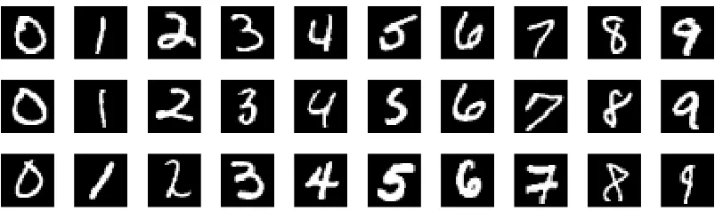
Figure 1: Sample images from the MNIST data set, with gray-scale from 0 to 255.
We can also restrictℓ1-regularization on part of the optimization variables only. For example,
in support vector machines or logistic regression, we usually want the bias terms to be free of
regularization. In this case, we can simply replaceλRDAt by 0 for the corresponding coordinates
in (30).
6.2 Experiments on the MNIST Data Set
Each image in the MNIST data set is represented by a 28×28 gray-scale pixel-map, for a total of
784 features. Each of the 10 digits has roughly 6,000 training examples and 1,000 testing examples. Some of the samples are shown in Figure 1. From the perspective of using stochastic and online algorithms, the number of features and size of the data set are considered very small. Nevertheless, we choose this data set because the computational results are easy to visualize. No preprocessing of the data is employed.
We use ℓ1-regularized logistic regression to do binary classification on each of the 45 pairs
of digits. More specifically, let z= (x,y) where x∈R784 represents a gray-scale image and y∈
{+1,−1} is the binary label, and let w= (w˜,b)where ˜w∈R784 and b is the bias. Then the loss
function and regularization term in (1) are
f(w,z) =log 1+exp −y(w˜Tx+b)
, Ψ(w) =λkw˜k1.
Note that we do not apply regularization on the bias term b. In the experiments, we compare the
(enhanced)ℓ1-RDA method (Algorithm 2) with the SGD method
wt(i+)1=wt(i)−αt
g(ti)+λsgn(w
(i)
t )
, i=1, . . . ,n,
and the TG method (29) withθ=∞. These three online algorithms have similar convergence rates
and the same order of computational cost per iteration. We also compare them with the batch optimization approach, more specifically solving the empirical minimization problem (2) using an efficient interior-point method (IPM) of Koh et al. (2007).
Each pair of digits have about 12,000 training examples and 2,000 testing examples. We use online algorithms to go through the (randomly permuted) data only once, therefore the algorithms
stop at T =12,000. We vary the regularization parameter λfrom 0.01 to 10. As a reference, the
maximumλfor the batch optimization case (Koh et al., 2007) is mostly in the range of 30−50
λ=0.01 λ=0.03 λ=0.1 λ=0.3 λ=1 λ=3 λ=10
SGD
TG
RDA
IPM
SGD
TG
RDA
wT
wT
wT
w⋆
¯
wT
¯
wT
¯
wT
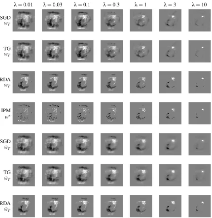
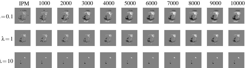
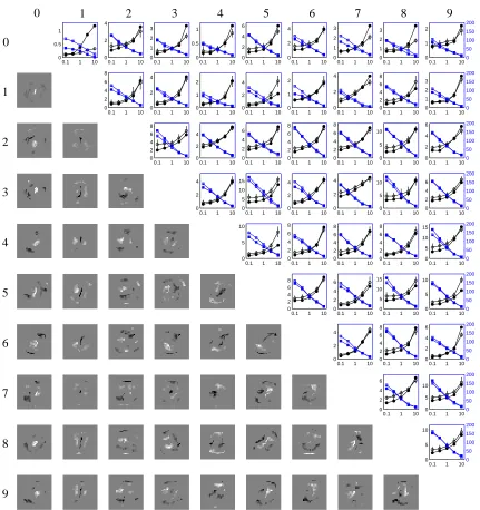
Figure 2: Sparsity patterns of wT and ¯wT for classifying the digits 6 and 7 when varying the
pa-rameter λfrom 0.01 to 10 in ℓ1-regularized logistic regression. The background gray
represents the value zero, bright spots represent positive values and dark spots represent
negative values. Each column corresponds to a value ofλ labeled at the top. The top
three rows are the weights wT (without averaging) from the last iteration of the three
online algorithms; the middle row shows optimal solutions of the batch optimization problem solved by interior-point method (IPM); the bottom three rows show the averaged
weights ¯wT in the three online algorithms. Both the TG and RDA methods were run with
0 2000 4000 6000 8000 10000 12000 0
100 200 300 400 500 600
0 2000 4000 6000 8000 10000 12000 0
100 200 300 400 500 600
0 2000 4000 6000 8000 10000 12000 0
100 200 300 400 500 600
0 2000 4000 6000 8000 10000 12000 0
100 200 300 400 500 600
SGD SGD
TG (K=1) RDA (ρ=0)
TG (K=10) RDA (γρ=25)
Number of samples t Number of samples t
N
N
Z
s
in
wt
(
λ
=
0
.
1
)
N
N
Z
s
in
wt
(
λ
=
1
0
)
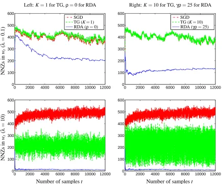
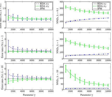
Left: K=1 for TG,ρ=0 for RDA Right: K=10 for TG,γρ=25 for RDA
Figure 3: Number of non-zeros (NNZs) in wt for the three online algorithms (classifying the pair 6
and 7). The left column shows SGD, TG with K =1, and RDA withρ=0; the right
column shows SGD, TG with K=10, and RDA withγρ=25. The same curves for SGD
are plotted in both columns for clear comparison. The two rows correspond toλ=0.1
andλ=10, respectively.
be either 0 for basic regularization, or 0.005 (effectivelyγρ=25) for enhanced regularization effect.
These parameters are chosen by cross-validation. For the SGD and TG methods, we use a constant
stepsizeα= (1/γ)p2/T for comparable convergence rate; see (19) and related discussions. In the
TG method, the period K is set to be either 1 for basic regularization (same as FOBOS), or 10 for
periodic enhanced regularization effect.
Figure 2 shows the sparsity patterns of the solutions wT and ¯wTfor classifying the digits 6 and 7.
The algorithmic parameters used are: K=10 for the TG method, andγρ=25 for the RDA method.
It is clear that the RDA method gives more sparse solutions than both SGD and TG methods. The sparsity pattern obtained by the RDA method is very similar to the batch optimization results solved
0.01 0.1 1 10 0.1
1 10
0.01 0.1 1 10
0 1 2 3 4
0.01 0.1 1 10
0 200 400 600
0.01 0.1 1 10
0 200 400 600
0.01 0.1 1 10
0.1 1 10
0.01 0.1 1 10
0 1 2 3 4
0.01 0.1 1 10
0 200 400 600
0.01 0.1 1 10
0 200 400 600
Regularization parameterλ
Regularization parameterλ
E
rr
o
r
ra
te
s
o
f
wT
(%
)
E
rr
o
r
ra
te
s
o
f
¯wT
(%
)
N
N
Z
s
in
wT
N
N
Z
s
in
¯wT
SGD SGD
TG (K=1) RDA (ρ=0)
TG (K=10) RDA (γρ=25) IPM
IPM
Left: K=1 for TG,ρ=0 for RDA Right: K=10 for TG,γρ=25 for RDA
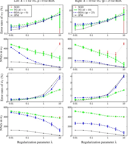
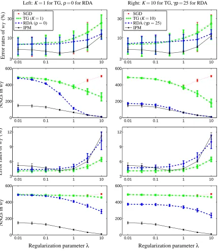
Figure 4: Tradeoffs between testing error rates and NNZs in solutions when varyingλfrom 0.01
to 10 (for classifying 6 and 7). The left column shows SGD, TG with K=1, RDA with
ρ=0, and IPM. The right column shows SGD, TG with K=10, RDA withγρ=25, and
IPM. The same curves for SGD and IPM are plotted in both columns for clear comparison.
The top two rows shows the testing error rates and NNZs of the final weights wT, and the
bottom two rows are for the averaged weights ¯wT. All horizontal axes have logarithmic