Optimized ANFIS-Genetic Algorithm-Particle Swarm Optimization Model for Estimation of Side Orifices Discharge Coefficient

27

Numerical Methods in Civil Engineering

Optimized ANFIS-Genetic Algorithm-Particle Swarm Optimization

Model for Estimation of Side Orifices Discharge Coefficient

A. H. Azimi *, A. Rajabi**, S. Shabanlu***

ARTICLE INFO Article history: Received: January 2018. Revised: April 2018. Accepted: May 2018.

Keywords: Side orifice Open channel ANFIS

Genetic Algorithm Particle Swarm

Discharge coefficient

Abstract:

Generally, side orifices are installed on side walls of the main channels for regulating and controlling water. In this study, a novel hybrid model was developed in order to estimate discharge coefficient of circular and rectangular side orifices. The model was obtained using combination of ANFIS, Genetic Algorithm and Particle Swarm Optimization. Then, 6 different models were defined for each ANFIS and hybrid models. Also, Monte Carlo Simulations (MCs) were used to survey abilities of the numerical models. Additionally, k-fold cross validation (k=5) was employed to validate the numerical models. Next, using sensitivity analysis, the superior model and the most effective parameters were identified. The best model simulated the discharge coefficient using all input variables this with high accuracy. For instance, the correlation coefficient and scatter index for the model were computed 0.856 and 0.027, respectively. Furthermore, the dimensionless parameter “the ratio of height of the side orifice to the side orifice diameter (W/D) was identified as the most effective variable input.

D D

1. Introduction

A side orifice is installed on the side wall of the open channel to control and conduct excess water. Side orifices are widely employed for flow distribution in irrigation channels, drainage networks and urban sewage disposal systems. The hydraulics of the flow passing through side weirs have been studied by numerous researchers.

For instance, Ramamurthy et al. (1986) [1] was one of the first ones who conducted an experimental study on the behavior of the flow passing through side orifices. They proposed a relationship as a function of hydraulic and geometric characteristics of the side orifice and the main channel for calculating the discharge coefficient of rectangular side orifices. Also, other researchers such as Gill (1987) [2], Swamee et al. (1993) [3], Ojha and Subbaiah (1997) [4] and Oliveto et al. (1997) [5] carried out studies on the passing flow through divert structures.

* Ph.D. Candidate, Department of Water Engineering, Kermanshah Branch, Islamic Azad University, Kermanshah, Iran.

**Corresponding Author: Assistant Professor, Department of Water Engineering, Kermanshah Branch, Islamic Azad University, Kermanshah, Iran. ([email protected])

***Associate Professor, Department of Water Engineering, Kermanshah Branch, Islamic Azad University, Kermanshah, Iran.

Hussein et al. (2010) [6] experimentally investigated the discharge capacity of circular side orifices located on the side wall of a rectangular channel in subcritical flow regime. They concluded a formula for computing the discharge coefficient of sharp-edged side orifices. Their suggested equation was a function of Froude number and the ratio of the side orifice diameter to the width of the main channel. Hussein et al. (2011) [7] studied the hydraulics of the flow passing through rectangular side orifices. They investigated the discharge capacity, velocity vectors and flow lines in the vicinity of rectangular sharp-crested side orifices in subcritical flow conditions. They also proposed a relationship as a function of hydraulic and geometric characteristics of the main channel and the side orifice. Hussein et al. (2014) [8] suggested a series of analytical relationships for calculating discharge passing through side orifices.

In recent years, various artificial intelligence algorithms as well as soft computation methods have been used in modeling irregular and complex phenomena in different sciences. For example, Bagheri et al. (2014) [9] simulated the discharge coefficient of rectangular side weirs in subcritical flow conditions using the artificial neural network. They carried out a sensitivity analysis to examine the influence of different parameters on the discharge

Numerical Methods in Civil Engineering, Vol. 2, No. 4, June. 2018 coefficient of such structures. They exhibited that Froude number is the most effective parameter affecting the discharge coefficient of rectangular side weirs. In addition, Zaji et al. (2014) [11] modeled the discharge coefficient of triangular side weirs by means of various neural networks and the particle swarm optimization algorithm. By analyzing the results of the numerical models, they stated that the particle swarm optimization algorithm models value of discharge coefficient exhibited higher accuracy. The maximum error value for the best model in their study was predicted to be approximately 0.041. Consequently, Ebtehaj et al. (2015) [10] modeled the discharge capacity of rectangular side orifices using the GMDH method. They considered the influence of hydraulic and geometric parameters in order to forecast the discharge coefficient of side orifices and finally developed five different models. By analyzing the modeling results, they demonstrated that the model which considers the influence of all input parameters had higher accuracy. Aydin and Kayisli (2016) [11] evaluated the discharge coefficient of labyrinth side weirs with two cycles in an artificial intelligence study using the ANFIS model. They compared the ANFIS model with a non-linear regression model and stated that the ANFIS model estimated the discharge coefficient of weirs with higher accuracy. Khoshbin et al. (2016) [12] simulated the discharge capacity of rectangular side weirs under subcritical flow conditions by means of ANFIS, the Genetic Algorithm and singular value. Using the parameters affecting the discharge coefficient, they proposed several models to predict the coefficient. By examining the results, they also indicated that the Froude number, the ratio of weir length to upstream depth and the ratio of side weir length to main channel width are the most effective factors.

Related to the nobility, quality and credibility of the study, it should be stated that the application of artificial intelligence (AI) methods has increasingly developed and these approaches are extensively applied in various fields to simulate complex and nonlinear problems [13-15].

On the other hand, the determination of the discharge coefficient of rectangular and circular side orifices is crucially important, meaning that the discharge coefficient of a side orifice is one of the most significant factors to provide an efficient, cost-effective and safe design.

Regarding the literature, there is no study to simulate discharge coefficient of both rectangular and circular side orifices by using a meta-heuristic AI model. This means that combination of the ANFIS network with two optimization techniques including the genetic algorithm (GA) and the particle swarm optimization (PSO) algorithm and subsequently, developing ANFIS-PSOGA, is applied to estimate the discharge coefficient of the rectangular and circular side orifices for the first time.

To this end, the discharge coefficient of circular and rectangular side orifices is simulated by the ANFIS-PSOGA meta-heuristic AI approach. Next, different ANFIS-PSOGA models are developed using the input parameters and then the superior model as well as the most effective parameters are detected using a sensitivity analysis.

2. Material and Methods

2.1 Adaptive Neuro-Fuzzy Inference System (ANFIS)

For the first time, ANFIS was provided by Jang (1993) [16] in the framework of an adaptive neural network. The structure of an adaptive neural network consists of a number of nodes in different layers connected to each other. The output of this network depends on adjustable parameters in nodes. The learning rules of the network determine how parameters should be updated in order to minimize the error value. The structure of a fuzzy inference system consists of three main components: the rules base, the database, and a logic mechanism. The rules base includes if-then rules. For example, "if the value of x is small, then y decreases" could be a fuzzy rule, so that "low" and "high" in this rule are verbal variables. The rules base performs membership functions used in fuzzy rules and the logic mechanism performs conclusion procedure from input variables. It is assumed that the fuzzy system has two variables x and y and an output z. In addition, the rules base consists of two if-then fuzzy rules in the first-order Takagi-Sugeno fuzzy system as follows:

(1)

(2)

The structure of ANFIS consists of five different layers defined as follows (Jang, 1993) [16]:

Layer1: Nodes in this layer are adaptive nodes and the output of each node is calculated as follows:

( )

i A i,

1 =μ (3)

Where, x is the input value of the node Ai and O1,I is the

membership function of the linguistic variable Ai.

There are different shapes for the membership function A. However, considering the good performance of bell-shaped membership functions in different studies, the employed function is defined as follows:

( )

Where, ai, bi and ci are function parameters. By changing any

of these parameters, the bell-shaped membership function also changes, generating various forms of the membership function for the fuzzy set. Parameters existing in this layer are introduced as premise parameters. These parameters are set during the learning process.

1 1 1 1 1

1 y B f px qy r

A

xis and is then   

if : Rule1 2 2 2 2 2

2 y B f px q y r

A x

:if is and is then   

Rule2

29

Layer2: The value of each node in this layer which denotes the output intensity or the firing strength is the ith rule and is constant. The output of this layer is the product of the signals of all inputs, which can be calculated as follows:

(5)

Layer3: each node in this layer is fixed. In this layer, the ratio of the ith rule intensity to the total of all rules is computed as follows:

(6)

Layer4: Nodes in this layer run the output of each layer:

(

p

x

q

y

r

)

i

12

w

f

w

O

=

=

+

+

=

Where, rj, qi and pi are tally parameters.

Layer5: In this layer, there is only one node which is a fixed node and shows the final value of the output parameter as a total of all input signals as follows:

i i i i i i , 5 w f w f w

O =

∑

∑

The ANFIS training phase is conducted to adjust all adjustable parameters (membership function parameters) in order to obtain output values of the ANFIS system with the maximum accommodation of learning data. After training ANFIS, the output can be obtained by introducing different input data. Assuming the parameters of the target function to be constant, the ANFIS output can be calculated by using the following relationship (Jang, 1997) [16]:

(

)

(

)

1 2 2 1 2 1 2 1 1 r y q x p w r y q x p w f w w w f w w w f + + + + + = + + + = ₍₉₎

In fact, f is a linear combination of the tally parameters (p1,

q1, r1, p2, q2, r2).

There are different algorithms for training ANFIS. Back-propagation and hybrid (a combination of the back-propagation and least square) algorithms are two common types. However, due to the weak performance of gradient-based algorithms in solving complex problems, in this study, the genetic algorithm as one of the most powerful optimization algorithms in various engineering problems is employed to optimal adjustment of membership function parameters.

2.2 Genetic Algorithm

The Genetic Algorithm (Holland 1975 [17]) is a comprehensive probabilistic search method that follows the natural regimen of evolution. This algorithm operates on the population of potential responses and uses the principle of survival struggle in generating better approximations of the problem. In each generation, a new set of approximations is constructed with the process of selecting the best member

based on their fitting in the domain of amplitude and propagation with operators derived from natural genetics. This process ultimately ends in the evolution of a population of members that are better adapted to the environment than the original members, which are in fact their parent. The general description of the genetic algorithm is as follows: 1- Start: Create a population of n chromosomes (potential problem answers) randomly

2- Fitness: Assess the fitness of each chromosome-x with the use of the fitness function x.

3. New population: Create new stages by repeating the steps below until new completion

3-1. Selection: Selecting two mother chromosomes from the population based on their compatibility

3-2. Cross-over: The mother's chromosomes of Step 3-1 mate randomly, with the determined probability level, and produce two offspring. If the cross-over does not take place, the offspring will be identical to the two chromosomes of the mother.

3.3. Mutation: The offspring chromosomes are motivated randomly with a certain probability level.

3-4 Offspring created using the genetic operators (selection, crossover and mutation) are placed in the new population. 4. Replacement: from the population produced are placed in the new population.

5. Convergence condition: If the desired conditions such as achieving the desired accuracy or the number of repetitions specified in the problem are obtained, the algorithm stops and the existing population shows the optimal response. 6. Repeat loop: If the algorithm does not stop in step 5, we go back to step 2 and repeat the process until it reaches the desired condition. In this research, the initial population is 30, the number of generations is 1000, the cross-over constant is equal to 0.8, the mutation constant is considered equal to 0.02. The intersection method has been used as a two-point crossover and the roulette wheel method has been used for selection. The stop criterion is considered to be a non-progressive function for 70 consecutive generations or ending the number of generations. Also, to replace newborn offspring with the population of the previous generation, the fitness function related to a particle of chromosomes is evaluated, and those who are more qualified are selected as the alternative population.

2.3 Particle Swarm Optimization (PSO)

PSO, is a meta-heuristic approach introduced by Eberhart and Kennedy (1995) [18], is a member of evolutionary algorithms that inspired the social behavior of particles like birds and fish in finding food resources. PSO provides the possibility of local and global search and fast convergence to global optimization by adjusting simple parameters. The main advantage of this method over other minimization strategies is that abundant amount of swarming particles that

2

,

1

)

(

).

(

2



w



x

x

i



O

i





2 , 1 2 1 1 ,

3   _ i

w w

w w O _{i i}

Numerical Methods in Civil Engineering, Vol. 2, No. 4, June. 2018 makes this method stable against the local minimizing problem.

In this algorithm, first, an initial response set is created. Then, for finding the optimized response in the possible response space, a response search is conducted by updating generations. Each particle is defined as two-dimensional with two situations and velocity values and in each step of particle movement the best response in terms of fitness is determined for all particles. The best situation obtained in each step is known as pbest and the end of all steps is known as gbest. All particles obtained based on pbest and gbest, update their situations to achieve the global optimized solution. Assuming x as the location of ith particle and v as its velocity, the velocity and location of each particle at each iteration is calculated and updated by the following relationships:

( ) ( ) ( )

( )

(

)

( )

(

)

rand . c t v . t w 1 t

i 2

i

1 i i

+ + =

+

ν (10)

(11)

Where, t=1,2,…,Imax-1, i=1,2,…,N represents the number of

iteration, Imax is the maximum iteration, rand() produces a

random value on the domain [0 1), c1 and c2 are two positive

constant values entitled "cognition learning rate" and "social learning rate" and their best case is when the sum of them is at least equal to 4. In this study, both values of c1 and c2 in

the optimized case are considered equal to 2.05. pbest(t) is the best response obtained in the tth iteration and gbest(t) is

the best response obtained until the tth iteration.w(t) is inertia

weight calculated by the following relationship:

 





max min max max

I

t w w w t

w     (12)

Where, wmin and wmax are the minimum and maximum

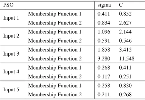
inertia weights, which in this study are taken into account as equal to 0.3 and 0.9, respectively. In Table 1, the Optimized parameters of Guassian function for particle swarm optimization algorithm is tabulated.

Table 1: Optimized parameters of Guassian function for PSO algorithm

PSO sigma C

Input 1 Membership Function 1 0.411 0.852

Membership Function 2 0.834 2.627

Input 2 Membership Function 1 1.096 2.144

Membership Function 2 0.591 0.546

Input 3 Membership Function 1 1.858 3.412

Membership Function 2 3.280 11.548

Input 4 Membership Function 1 0.268 0.411

Membership Function 2 0.117 0.251

Input 5 Membership Function 1 0.258 0.830

Membership Function 2 0.211 0.268

2.4 Hybrid Algorithm

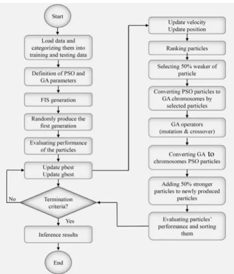
Genetic algorithms and PSO have many similarities such as being meta-heuristic and evolutionary and are able to search based on the population. In fact, in each iteration, in order to reach the optimal global, both algorithms using a series of actual and probability rules move from a set called “population” towards other points. Each method has different advantages and disadvantages as well. GA has a high computational cost due to its high dependence on genetic operators such as crossover, mutation and selection as well as its need to evaluate numerous functions during each iteration. The PSO algorithm has memory, and if an individual is not selected during the selection process, its information is removed. In addition, as GA is not powerful in finding an accurate response, its best function is to estimate an optimal global region. In PSO, mutual group interactions increase the speed to obtain the optimal response. However, due to the lack of the selection operator, PSO might waste many resources on a weak individual located at a long distance from the optimal response. In this paper, a hybrid algorithm entitled “PSOGA” is provided, which has the influence on GA and PSO algorithms for increasing accuracy in the search environment. In this algorithm, GA is used to increase the accuracy of the PSO performance by providing a space for data interchange. The main aim of this method is to reach the optimal global considering the whole search space, so that speed and position rules in the PSO algorithm are updated by the crossover, mutation and selection operators. Thus, some individuals in the previous generation are similar to each other with the exception that, based on the PSO algorithm, they are placed in various locations of the search space and other individuals are replaced by individuals produced by genetic operators. Also, a flowchart of the hybrid model is depicted in Figure 1.

)

1

(

)

(

)

1

(

t





x

t



v

t



x

31

2.5 Experimental Model

In this study, the experimental measurements done by Hussein et al. (2010) [6] and Hussein et al. (2011) [7] are employed to verify the results of the numerical model. Their experimental model is composed of an open rectangular channel with the length, width and height of 9.15m, 0.5m and 0.6m, respectively. A slide gate installed at the end of the system is utilized to adjust the flow depth in the mentioned channel. Hussein et al. (2011) [7] calculated the values of Qm, Q, D, Ym, V1, W and Fr as discharge in the main

channel, discharge passing through the side orifice, the side orifice dimension, the flow depth in the main channel, flow velocity in the main channel, the elevation of the side orifice bed from the channel bed and the Froude number in the main channel. The experimental model used by Hussein et al. is shown in Figure 2.

Fig. 2: Experimental model used by Hussein et al. (2010) and (2011) for circular and rectangular side orifices

2.6 Discharge coefficient of Side Orifices

Hussein et al. (2010) [6] and Hussein et al. (2011) [7] considered the discharge capacity of rectangular side

orifices as a function of length and width of the rectangular side orifice with circular diameter (D), width of the main channel (B), the elevation of the side orifice bed from the main channel bed (W), flow velocity in the main channel (V1), the flow depth in the main channel (Ym), density of fluid

(ρ), viscosity of flow (μ) and the gravitational acceleration (g):

(13)

Considering the flow Froude number is Fr=V1/√(g.Ym),

values of density, viscosity and the gravitational acceleration are taken into account and also values of B, W and Ym to

length of the side orifice are made dimensionless. Therefore, Equation (13) is written as follows:

(14)

In addition, in this study, the influence of the shape of the side orifice is also investigated. To consider the effects of the side orifice shape, the parameter φ is introduced. For a rectangular side orifice, the value of φ is equal to 1 and for a circular side orifice this value is considered 2. Thus, the combination of input parameters is expressed as the following equation:

(15)

Thus, for modeling the discharge coefficient of side orifices, the dimensionless parameters involved in Equation 15 are implemented. In Figure 3, the combinations of different artificial intelligence models are illustrated in two cases including No.1 and No.2. These two different combinations are employed to identify the influence of the shape factor in modeling the discharge coefficient. In order to detect the most effective input factor in each of the different combinations, the influence of different input parameters is removed one by one and the modeling process is run.

Fig. 3: Schematic of different artificial intelligence models

Moreover, in this study the Monte Carlo simulations are used for examining the abilities of the artificial intelligence models. The Monte Carlo simulation is a broad classification of computational algorithms which uses random sampling



L

b

B

W

V

Y

g



f

C



,

,

,

,

,

,



,



,















m

d

F

D

Y

D

W

D

B

f

C

,

,

,















,

,

,

,



m

d

F

D

Y

D

W

D

B

f

C

Numerical Methods in Civil Engineering, Vol. 2, No. 4, June. 2018 for calculating numerical results. The main idea of this approach relies on the basis that, using random decision-making tries to solve problems which might be real in nature. The Monte-Carlo methods are usually implemented for simulating physical and mathematical systems which are not solvable by means of other methods. The Monte Carlo simulation is generally employed using the probability distribution for solving various problems such as optimization and numerical integration. Furthermore, the k-fold cross validation method is utilized to examine the proficiency of the mentioned models. In the k-fold cross validation method, the main sample is divided into k samples with the same size randomly. Among k sub-samples, one sub-sample is used as the validation data and the remaining as the train data of the model. Then, the method repeats k times (equal to the number of layers), so that each k sub-sample is used exactly once as the validation data. The results obtained from the mentioned k layers are averaged and provided as an approximation. The advantage of this method is the random repetition of sub-samples in the test and learning process for all observations and each observation is exactly used once as the validation data. In this paper, the k value is assumed as 5. The schematic of the k-fold cross validation method is illustrated in Fig 4. It should be stated that the number of all experimental data used is about 380.

Fig. 4: Schematic layout of the k-fold cross validation method

3. Results and Discussion

3.1 Criteria for examining accuracy of numerical

models

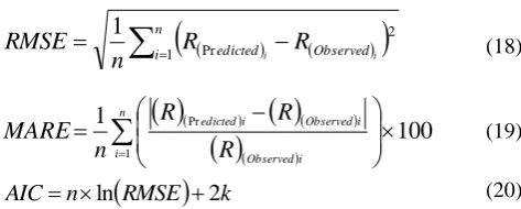
In this study, the statistical indices including correlation coefficient (R), variance accounted for (VAF), root mean square error (RMSE), mean absolute relative error (MARE) and Akaike information criterion (AIC) are used as follows:

(16)

(17)

(18)

(19)





AIC ln 2 (20)

In these equations, the values of (R)(Observed)i, (R)(Predicted)i,

and n are experimental data, results predicted by numerical models, the average of experimental data and the number of experimental measurements. Also, k denotes the number of estimated parameters included in each model.

3.2 Study of different generations of Fuzzy-Inference

system

The ANFIS network has three different Fuzzy-Inference systems and the most optimized generation should be chosen for estimating the discharge coefficient of side orifices and carried out in the following sentences. In Figures 5 and 6, the comparison of different statistical indices for three generations of fuzzy inference system and the comparison of simulated and observed values are respectively shown. Based on the review, three generations of the fuzzy inference systems are: Grid Partitioning (GP), Subtractive Clustering (SC) and Fuzzy C-Means Clustering (FCM). According to the numerical modeling results, the Fuzzy C-Means Clustering generation has higher accuracy compared to two other generations. For example, the correlation coefficient for this generation is 0.683, while the value of VAF is calculated 42.629. In addition, for FCM, the values of RMSE and MARE are 0.024 and 0.025, respectively. For the GP and SC generations, the scatter index is computed equal to 0.038. For GP, the values of R, RMSE and MARE obtained are 0.677, 0.024 and 0.026, respectively. Based on the results of the discharge coefficient simulated by different generations of fuzzy inference system, it is observed that the FCM generation simulates these values with higher accuracy. Thus, in the following, this generation is used for modeling discharge coefficient values of rectangular and circular side orifices.

 

 







 

 



 

 







 

 



















i edictedi edicted Observed

i Observed n

i Observedi Observed edictedi edicted

R

R

R

R

R

R

R

R

R

1 Pr Pr





100

var

var

1

VAF

























R

R

R











i

R

R

n

RMSE

1

 

 

 

100

1























_

i _Observedi

i Observed i edicted

R

R

R

n

MARE

 

R

33

generations of fuzzy inference system

Fig. 6: Comparison of observed and simulated discharge coefficient

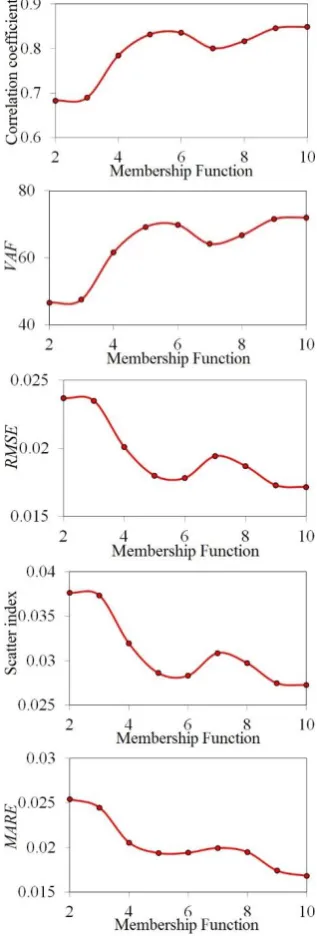
3.3 Selection of optimized membership function

In modeling different non-linear phenomena by the ANFIS network, the selection of the membership function is very important. In this section, the membership functions are evaluated. The results of different statistical indices for changes of the membership functions are shown in Figure 7. As shown, the first membership function is chosen equal to 2. As the value of this function increases, the correlation

coefficient also increases whereas the error value decreases. For example, in this study, the number of the optimized membership functions is considered 5. The values of R, VAF and RMSE for this optimized membership function are computed 0.832, 69.186 and 0.018, respectively. Also, MARE obtained for this membership function is 0.019, respectively.

Fig. 7: Changes of membership functions versus different statistical indices

3.4 ANFIS Models

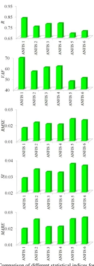
In this study, six ANFIS models and six ANFIS-PSOGA models are defined. At the beginning, the ANFIS models are examined. To identify the most effective parameter, a sensitivity analysis is used. To this end, ANFIS1 is a function of all input parameters and ANFIS2 to ANFIS6 are

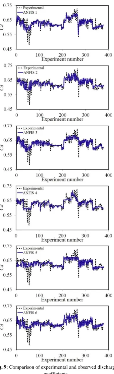
Numerical Methods in Civil Engineering, Vol. 2, No. 4, June. 2018 developed through the elimination of a parameter. The results of different statistical indices for the ANFIS models are illustrated in Figure 8 and Table 2. Furthermore, the comparison of the numerical and experimental values obtained from these models is shown in Figure 9. For example, the ANFIS1 model simulates values of the discharge coefficient in terms of all input parameters. For the ANFIS1 model, the values of R and VAF are calculated 0.832 and 69.186, respectively. In addition, the values of RMSE and MARE for the mentioned model are 0.018 and 0.019, respectively. For the ANFIS2 model, the shape parameter (φ) is eliminated and this model simulates values of the discharge coefficient in terms of B/D, W/D, Ym/D, Fr.

For this model, the values of RMSE, MARE and AIC are computed 0.021, 0.025 and -1132.66, respectively. For simulating the discharge coefficient of side orifices by ANFIS3, the influence of Fr is neglected. In other words, this

model is a function of B/D, W/D, Ym/D, φ. For this model,

the R and AIC statistical indices are calculated 0.777 and -1147.39, respectively. ANFIS4 simulates values of the discharge coefficient in terms of B/D, W/D, φ, Fr and the

influence of the parameter Ym/D is removed for this model.

For ANFIS4, the values of the correlation coefficient and the scatter index are calculated 0.783 and 0.032, respectively. As shown, among the models with four input parameters, this model estimates the discharge coefficient with higher accuracy. Furthermore, the values of MARE and AIC for the mentioned model are 0.021 and -1151.52, respectively. For ANFIS5, the influence of the parameter W/D is neglected. In other words, this model estimates objective function values in terms of B/D, φ, Ym/D, Fr. According to the modeling

results, this model has the lowest accuracy among all ANFIS models. For example, the values of MARE and AIC for the mentioned model are 0.025 and -1101.24, respectively. The values of R and RMSE for ANFIS5 are 0.689 and 0.024, respectively. The values of AIC and R for ANFIS6 are approximated -1111.05 and 0.710, respectively. This model calculates values of the discharge coefficient as a function of φ, W/D, Ym/D, Fr and the influence of the parameter B/D

is removed for this model. Furthermore, the values of RMSE and MARE for this model are calculated 0.023 and 0.026, respectively. Based on the ANFIS models, ANFIS1 has the highest accuracy and this model predicts values of the objective function with high accuracy. ANFIS1 is a function of all input parameters. In addition, according to the sensitivity analysis, the ratio of side orifice height from the channel bed to orifice dimensions (W/D) is detected as the most effective parameter.

Fig. 8: Comparison of different statistical indices for ANFIS models

Table 2: Results from ANFIS models

Models R VAF RMSE MARE AIC

ANFIS1 0.832 69.186 0.0184 0.019 -1188.94

ANFIS2 0.752 56.585 0.0214 0.025 -1132.66

ANFIS3 0.777 60.310 0.0204 0.020 -1147.39

ANFIS4 0.783 61.298 0.0201 0.021 -1151.52

ANFIS5 0.689 47.427 0.0235 0.025 -1101.24

ANFIS6 0.710 50.478 0.0228 0.026 -1111.05

35

coefficients

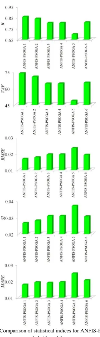
3.5 ANFIS-PSOGA Models

In the following, the ability of the hybrid models in estimating the discharge coefficient of rectangular and circular side orifices is evaluated. Similar to the previous case, the sensitivity analysis is carried out for identifying the superior model as well as the effective parameter. The results of different statistical indices for six hybrid models (ANFIS-PSOGA) are shown in Figure 10 and Table 3. In addition, the experimental and numerical values of the discharge coefficient are shown in Figure 11. According to the results obtained from the hybrid models, the values of the correlation coefficient, the scatter index and VAF for ANFIS-PSOGA 1 are 0.856, 0.027 and 73.356, respectively. For the mentioned model, RMSE and MARE are 0.017 and 0.018, respectively. However, among all numerical models, ANFIS-PSOGA 1 has the highest accuracy and the lowest error. ANFIS-PSOGA 2 has the highest accuracy among the models with four inputs. For this model, the value of VAF obtained is 70.353, respectively. In addition to these values, R, RMSE and MARE for the mentioned model are equal to 0.839, 0.018 and 0.019, respectively. Also, R and the scatter index for ANFIS-PSOGA 3 are 0.801 and 0.031, respectively. It should be noted that VAF and MARE for ANFIS-PSOGA 3 are 64.103 and 0.019, respectively. For ANFIS-PSOGA 4, the values of R and VAF are computed 0.801 and 64.129, respectively. The results of ANFIS-PSOGA 3 and ANFIS-ANFIS-PSOGA 4 are very close to each other. In other words, the performance of these two models is similar in approximating the discharge coefficient. The error value of RMSE for ANFIS-PSOGA 4 is calculated equal to 0.019. Also, the analysis of the results for ANFIS-PSOGA5 indicates that R and VAF are calculated 0.698 and 48.685, respectively. However, the values of RMSE and MARE for this hybrid model obtained are 0.023 and 0.025, respectively. Among all hybrid models, ANFIS-PSOGA 5 has the highest error. In addition, VAF for ANFIS-PSOGA 6 is computed equal to 64.916. The value of R for this model is equal to 0.806 and RMSE and MARE for ANFIS-PSOGA 6 are calculated as 0.019 and 0.020, respectively.

Numerical Methods in Civil Engineering, Vol. 2, No. 4, June. 2018

Fig. 10: Comparison of statistical indices for ANFIS-PSOGA hybrid models

Table 3: Results from ANFIS-PSOGA models

R VAF RMSE MARE AIC

ANFIS-PSOGA1 0.856 73.356 0.0167 0.018 -1505.96

ANFIS-PSOGA2 0.839 70.353 0.0177 0.019 -1471.28

ANFIS-PSOGA3 0.801 64.103 0.0194 0.019 -1310.41

ANFIS-PSOGA4 0.801 64.129 0.0194 0.019 -1383.84

ANFIS-PSOGA5 0.698 48.685 0.0232 0.025 -1294.09

ANFIS-PSOGA6 0.806 64.916 0.0192 0.020 -1415.02

Also, the MARE value for PSOGA 2, ANFIS-PSOGA 3 and ANFIS-ANFIS-PSOGA 4 is roughly 5% more than ANFIS-PSOGA 1, whilst the index for ANFIS-PSOGA 5 and ANFIS-PSOGA 6 is about 38% and 11% more than ANFIS-PSOGA 1, respectively.

Fig. 11: Comparison of observed discharge coefficient with discharge coefficient simulated by hybrid model

37

Based on the modeling results, ANFIS-PSOGA 1 which predicted the discharge coefficient values in terms of all input parameters is detected as the superior model, whereas by eliminating the ratio of the side orifice bed height from the channel bed to side orifice diameter (W/D), the error value significantly increases. Therefore, this input parameter is introduced as the most effective parameter.

In this section, a comparison between ANFIS, ANFIS-GA, ANFIS-PSO and ANFIS-PSOGA models is made. The results from the models are presented in Table 4. As it can be obviously seen, the ANFIS-PSOGA estimates the target function with better performance.

Table 4: comparison between ANFIS, ANFIS-GA, ANFIS-PSO and ANFIS-PSOGA models

Model R VAF RMSE MARE AIC

ANFIS 0.832 69.186 0.0184 0.019 -1188.943

ANFIS-GA 0.840 71.083 0.0176 0.018 -1407.934

ANFIS-PSO 0.837 70.495 0.0180 0.019 1322.783

ANFIS-PSOGA 0.856 73.356 0.00167 0.018

-1505.965

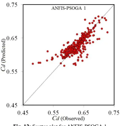
Moreover, a comparison between the superior model (ANFIS-PSOGA) with proposed model by Hussein et al. (2010), (2011) and Ebtehaj et al. (2015) is made. Maximum error for Hussein et al. (2010) and (2011) models was computed roughly as 5%, whilst the RMSE and MARE for Ebtehaj et al. (2015) model was calculated 0.021 and 0.019. Therefore, the ANFIS-PSOGA has higher accuracy in comparison to the previous studies. Then, the scatter plot for ANFIS-PSOGA 1 is depicted in Figure 12.

Fig. 12: Scatter plot for ANFIS-PSOGA 1

Generally, discharge coefficient is the most important parameter to design a side orifice. Thus, simulation of the parameters affecting the discharge coefficient can easily result in an optimized and cost-effective discharge capacity for the hydraulic structures. In the current study, an

optimized and accurate hybrid (ANFIS-PSOGA) model for estimating the discharge coefficient of rectangular and circular side orifices was presented. To do this, the ANFIS network was combined with two robust optimization algorithms including “genetic algorithm” (GA) and “particle swarm optimization” (PSO). Results showed that the optimization tools were quite beneficial in enhancing the ANFIS performance. Furthermore, through a sensitivity analysis, the superior hybrid model for estimating the discharge coefficient as well as the most influenced input parameter was introduced. The results may be quite beneficial for both scholars and engineers in practical usages.

4. Conclusions

A side orifice is an important and applicable hydraulic structure used in water transmission and control system. This structure is installed on the main channel wall, whose function is to conduct excess water to the outside of the channel once the elevation is above the weir crest. The main conclusions of this study are reported as follows:

The influence of all geometric and hydraulic parameters on the discharge coefficient was evaluated. The impact of the shape coefficient of the side orifice on the discharge coefficient was investigated. The Monte Carlo simulations were employed for examining the ability of the numerical models. The k-fold cross validation approach was utilized for verifying the results obtained from the numerical results. The k value in the k-fold cross validation method was considered equal to 5. The hybrid model was developed through the combination of the ANFIS network, GA and PSO. For each of ANFIS and ANFIS-PSOGA models, six different models were defined. For identifying the superior model and the effective parameter, a sensitivity analysis was used. The hybrid models simulated the discharge coefficient values with higher accuracy compared with the ANFIS models. The superior models of ANFIS and hybrid estimated the objective function values in terms of all input parameters. The ratio of the side orifice bed height from the channel bed to the side orifice diameter (W/D) was identified as the most effective parameter.

Finally, it was concluded that the developed hybrid artificial intelligence model simulated the discharge coefficient of side orifices, both rectangular and circular with reasonable accuracy. It should be noted that the model was quite optimum and flexible to estimate the target function because providing an efficient, reliable and cost effective discharge coefficient is absolutely important to design a side orifice. Therefore, scholars and engineers can gain a good insight into discharge coefficient of side orifices and its effective factors using the developed artificial intelligence technique.

Numerical Methods in Civil Engineering, Vol. 2, No. 4, June. 2018

References

[1] Ramamurthy, AS., Udoyara, ST., Serraf, S., “Rectangular

lateral orifices in open channel”, Journal of Environmental Engineering, Vol. 135(5), 1986, 292-298.

[2] Gill, MA., “Flow through side slots”, Journal of Environmental

Engineering, Vol. 135(21874), 1987, 1047-1057.

[3] Swamee, PK., Pathak, SK., Ali, MS., “Weir orifice units for

uniform flow distribution”, Journal of Irrigation and Drainage Engineering, Vol. 119(6), 1993, 1026-1035.

[4] Ojha, CSP., Subbaiah, D., “Analysis of flow through lateral

slot’, Irrigation and Drainage Engineering, Vol. 123(5), 1997, 402-405.

[5] Oliveto, G., Biggiero, V., Hager, WH., “Bottom outlet for

sewers”, Journal of Irrigation and Drainage Engineering, Vol. 123(4), 1997, 246-252.

[6] Hussein, A., Ahmad, Z., Asawa, GL., “Discharge

characteristics of sharp-crested circular side orifices in open channels”, Flow Measurement and Instrumentation, Vol. 21(3), 2010, 418-424.

[7] Hussein, A., Ahmad, Z., Asawa, GL., “Flow through

sharp-crested rectangular side orifices under free flow condition in open channels”, Agricultural Water Management, Vol. 98, 2011, 1536-1544.

[8] Hussein, A., Ahmad, Z., Ojha, CSP., “Analysis of flow through

lateral rectangular orifices in open channels”, Flow Measurement and Instrumentation, Vol. 36, 2014, 32-35.

[9] Bagheri, S., Kabiri-Samani, AR., Heidarpour, M., “Discharge

coefficient of rectangular sharp-crested side weirs, Part I:

traditional weir equation”, Flow Measurement and

Instrumentation, Vol. 35, 2014, 109-115.

[10] Ebtehaj, I., Bonakdari, H., Khoshbin, F., Azimi, H. “Pareto

genetic design of group method of data handling type neural network for prediction discharge coefficient in rectangular side orifices’’, Flow Measurement and Instrumentation, Vol. 41, 2015, 67-74.

[11] Aydin, MC., Kayisli, K., “Prediction of discharge capacity

over two-cycle labyrinth side weir using ANFIS”, Journal of Irrigation and Drainage Engineering, Vol. 142(5), 2016, 06016001.

[12] Khoshbin, F., Bonakdari, H., Ashraf Talesh, SH., Ebtehaj, I.,

Zaji, AH., Azimi, H., “Adaptive neuro-fuzzy inference system multi-objective optimization using the genetic algorithm/singular value decomposition method for modelling the discharge coefficient in rectangular sharp-crested side weirs’, Engineering Optimization, Vol. 48(6), 2016, 933-948.

[13] Akhbari, A., Zaji, A.H., Azimi, H., Vafaeifard, M., “Predicting the discharge coefficient of triangular plan form weirs using radian basis function and M5’methods”, Journal of Applied Research in Water and Wastewater, Vol. 4(1), 2017, 281-289.

[14] Azimi, H., Shabanlou, S., Ebtehaj, I., Bonakdari, H., Kardar,

S., “Combination of computational fluid dynamics, adaptive neuro-fuzzy inference system, and genetic algorithm for predicting discharge coefficient of rectangular side orifices”, Journal of Irrigation and Drainage Engineering, Vol. 143(7), 2017, 04017015. [15] Shabanlou, S., Azimi, H., Ebtehaj, I., Bonakdari, H., “Determining the scour dimensions around submerged vanes in a 180 bend with the gene expression programming technique”, Journal of Marine Science and Application, Vol. 17(2), 2018, 233-240.

[16] Jang, JS., “ANFIS: adaptive-network-based fuzzy inference

system”, IEEE Transactions on Systems, Man, and Cybernetics 20.03, 1993, 665-685.

[17] Holland, JH., “Adaptation in natural and artificial system’,

University of Michigan Press, Ann Arbor, 1975.

[18] Kennedy, J., Eberhart, R., “Particle swarm optimization”,

IEEE Int. Conf. Neural Networks, Vol. 4, 1995, 1942.1948.