Permutation Tests for Studying Classifier Performance

Permutation Tests for Studying Classifier Performance

Markus Ojala [email protected]

Helsinki Institute for Information Technology Department of Information and Computer Science Aalto University School of Science and Technology P.O. Box 15400, FI-00076 Aalto, Finland

Gemma C. Garriga [email protected]

Universit´e Pierre et Marie Curie Laboratoire d’Informatique de Paris 6 4 place Jussieu, 75005 Paris, France

Editor: Xiaotong Shen

Abstract

We explore the framework of permutation-based p-values for assessing the performance of classi-fiers. In this paper we study two simple permutation tests. The first test assess whether the classifier has found a real class structure in the data; the corresponding null distribution is estimated by per-muting the labels in the data. This test has been used extensively in classification problems in computational biology. The second test studies whether the classifier is exploiting the dependency between the features in classification; the corresponding null distribution is estimated by permut-ing the features within classes, inspired by restricted randomization techniques traditionally used in statistics. This new test can serve to identify descriptive features which can be valuable infor-mation in improving the classifier performance. We study the properties of these tests and present an extensive empirical evaluation on real and synthetic data. Our analysis shows that studying the classifier performance via permutation tests is effective. In particular, the restricted permutation test clearly reveals whether the classifier exploits the interdependency between the features in the data.

Keywords: classification, labeled data, permutation tests, restricted randomization, significance

testing

1. Introduction

Building effective classification systems is a central task in data mining and machine learning. Usually, a classification algorithm builds a model from a given set of data records in which the labels are known, and later, the learned model is used to assign labels to new data points. Applications of such classification setting abound in many fields, for instance, in text categorization, fraud detection, optical character recognition, or medical diagnosis, to cite some.

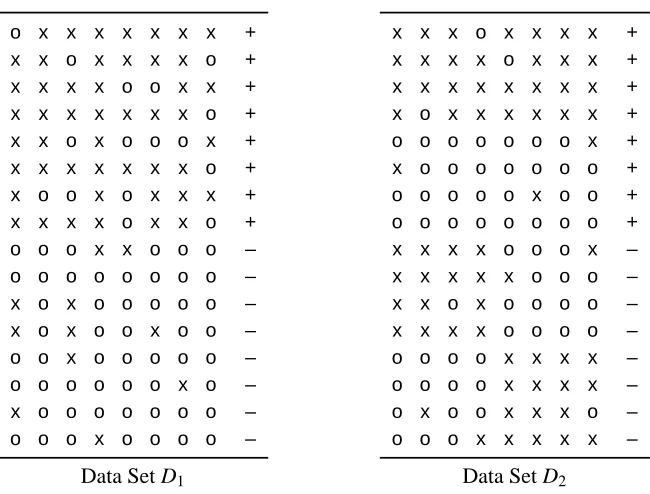
o x x x x x x x +

x x o x x x x o +

x x x x o o x x +

x x x x x x x o +

x x o x o o o x +

x x x x x x x o +

x o o x o x x x +

x x x x o x x o +

o o o x x o o o –

o o o o o o o o –

x o x o o o o o –

x o x o o x o o –

o o x o o o o o –

o o o o o o x o –

x o o o o o o o –

o o o x o o o o –

Data Set D1

x x x o x x x x +

x x x x o x x x +

x x x x x x x x +

x o x x x x x x +

o o o o o o o x +

x o o o o o o o +

o o o o o x o o +

o o o o o o o o +

x x x x o o o x –

x x x x x o o o –

x x o x o o o o –

x x x x o o o o –

o o o o x x x x –

o o o o x x x x –

o x o o x x x o –

o o o x x x x x –

Data Set D2

Figure 1: Examples of two 16_×8 nominal data sets D1 and D2each having two classes. The last

column in both data sets denotes the class labels (+,–) of the samples in the rows.

dimensionality (thousands of features) and small number of data points (tens of rows). An important question is whether we should believe in the classification accuracy obtained by such classifiers.

The most traditional approach to this problem is to estimate the error of the classifier by means of cross-validation or leave-one-out cross-validation, among others. This estimate, together with a variance-based bound, provides an interval for the expected error of the classifier. The error estimate itself is the best statistics when different classifiers are compared against each other (Hsing et al., 2003). However, it has been argued that evaluating a single classifier with an error measurement is ineffective for small amount of data samples (Braga-Neto and Dougherty, 2004; Golland et al., 2005; Isaksson et al., 2008). Also classical generalization bounds are not directly appropriate when the dimensionality of the data is too high; for these reasons, some recent approaches using filtering and regularization alleviate this problem (Rossi and Villa, 2006; Berlinet et al., 2008). Indeed, for many other general cases, it is useful to have other statistics associated to the error in order to understand better the behavior of the classifier. For example, even if a classification algorithm produces a classifier with low error, the data itself may have no structure. Thus the question is, how can we trust that the classifier has learned a significant predictive pattern in the data and that the chosen classifier is appropriate for the specific classification task?

For instance, consider the small toy example in Figure 1. There are two nominal data matrices

D1 and D2 of sizes 16×8. Each row (data point) has two different values present, xando. Both

data sets have a clear separation into the two given classes,+and–. However, it seems at first sight that the structure within the classes for data set D1is much simpler than for data set D2. If we train

a 1-Nearest Neighbor classifier on the data sets of Figure 1, we have that the classification error (leave-one-out cross-validation) is 0.00 on both D1and D2. However, is it true that the classifier is

some simple structure? It turns out that the good classification result in D1is explained purely by

the different value distributions inside the classes whereas in D2 the interdependency between the

features is important in classification. This example will be analyzed in detail later on in Section 3.3. In recent years, a number of papers have suggested to use permutation-based p-values for as-sessing the competence of a classifier (Golland and Fischl, 2003; Golland et al., 2005; Hsing et al., 2003; Jensen, 1992; Molinaro et al., 2005). Essentially, the permutation test procedure measures how likely the observed accuracy would be obtained by chance. A p-value represents the fraction of random data sets under a certain null hypothesis where the classifier behaved as well as or better than in the original data.

Traditional permutation tests suggested in the recent literature study the null hypothesis that the features and the labels are independent, that is, that there is no difference between the classes. The null distribution under this null hypothesis is estimated by permuting the labels of the data set. This corresponds also to the most traditional statistical methods (Good, 2000), where the results on a control group are compared against the results on a treatment group. This simple test has been proven effective already for selecting relevant genes in small data samples (Maglietta et al., 2007) or for attribute selection in decision trees (Frank, 2000; Frank and Witten, 1998). However, the related literature has not performed extensive experimental studies for this traditional test in more general cases.

The goal of this paper is to study permutation tests for assessing the properties and performance of the classifiers. We first study the traditional permutation test for testing whether the classifier has found a real class structure, that is, a real connection between the data and the class labels. Our experimental studies suggest that this traditional null hypothesis leads to very low p-values, thus rendering the classifier significant most of the time even if the class structure is weak.

We then propose a test for studying whether the classifier is exploiting dependency between some features for improving the classification accuracy. This second test is inspired by restricted randomization techniques traditionally used in statistics (Good, 2000). We study its relation to the traditional method both analytically and empirically. This new test can serve as a method for obtaining descriptive properties for classifiers, namely whether the classifier is using the feature dependency in the classification or not. For example, many existing classification algorithms are like black boxes whose functionality is hard to interpret directly. In such cases, indirect methods are needed to get descriptive information for the obtained class structure in the data.

If the studied data set is known to contain useful feature dependencies that increase the class separation, this new test can be used to evaluate the classifier against this knowledge. For example, often the data is gathered by a domain expert having deeper knowledge of the inner structure of the data. If the classifier is not using a known useful dependency, the classifier performance could be improved. For example, with medical data, if we are predicting the blood pressure of a person based on the height and the weight of the individual, the dependency between these two features is important in the classification as large body mass index is known to be connected with high blood pressure. However, both weight and height convey information about the blood pressure but the dependency between them is the most important factor in describing the blood pressure. Of course, in this case we could introduce a new feature, the body mass index, but in general, this may not be practical; for example, introducing too many new features can make the classification ineffective or too time consuming.

the properties of the classifier, or it can guide the search towards an optimal classifier. For example, if the classifier is not exploiting the feature dependency, there might be no reason to use the chosen classifier as either more complex classifiers (if the data contains useful feature dependencies) or simpler classifiers (if the data does not contain useful feature dependencies) could perform better. Note, however, that not all feature dependencies are useful in predicting the class labels. Therefore, in the same way that traditional permutation tests have already been proven useful for selecting relevant features in some contexts as mentioned above (Maglietta et al., 2007; Frank, 2000; Frank and Witten, 1998), the new test can serve for selecting combinations of relevant features to boost the classifier performance for specific applications.

The idea is to provide users with practical p-values for the analysis of the classifier. The per-mutation tests provide useful statistics about the underlying reasons for the obtained classification result. Indeed, no test is better than the other, but all provide us with information about the classifier performance. Each p-value is a statistic about the classifier performance; each p-value depends on the original data (whether it contains some real structure or not) and the classifier (whether it is able to use certain structure in the data or not).

The remaining of the paper is organized as follows. In Section 2, we give the background to classifiers and permutation-test p-values, and discuss connections with previous related work. In Section 3, we describe two simple permutation methods and study their behavior on the small toy example in Figure 1. In Section 4, we analyze in detail the properties of the different permutations and the effect of the tests for synthetic data on four different classifiers. In Section 5, we give experimental results on various real data sets. Finally, Section 6 concludes the paper.1

2. Background

Let X be an n_×m data matrix. For example, in gene expression analysis the values of the matrix X

are numerical expression measurements, each row is a tissue sample and each column represents a gene. We denote the i-th row vector of X by Xiand the j-th column vector of X by Xj. Rows are also

called observations or data points, while columns are also called attributes or features. Observe that we do not restrict the data domain of X and therefore the scale of its attributes can be categorical or numerical.

Associated to the data points Xi we have a class label yi. We assume a finite set of known class

labels

Y

Y

example above, the class labels associated to each tissue sample could be, for example, “sick” or “healthy”.

In a traditional classification task the aim is to predict the label of new data points by training a classifier from D. The function learned by the classification algorithm is denoted by f :

X

Y

e(f,D) =1 n

n

∑

I(fD\Di(Xi)6=yi) (1)

where fD\Di is the function learned by the classification algorithm by removing the i-th observation

from the data and I(_·)is the indicator function.

It has been recently argued that evaluating the classifier with an error measurement is ineffective for small amount of data samples (Braga-Neto and Dougherty, 2004; Golland et al., 2005; Hsing et al., 2003; Isaksson et al., 2008). Also classical generalization bounds are inappropriate when the dimensionality of the data is too high. Indeed, for many other general cases, it is useful to have other statistics associated to the error e(f,D)in order to understand better the behavior of the classifier. For example, even if a consistent algorithm produces a classifier with low error, the data itself may have no structure.

Recently, a number of papers have suggested to use permutation-based p-values for assessing the competence of a classifier. Essentially, the permutation test procedure is used to obtain a p-value statistic from a null distribution of data samples, as described in Definition 1. In Section 3.1 we will introduce two different null hypotheses for the data.

Definition 1 (Permutation-based p-value) LetD be a set of k randomized versions Db ′of the orig-inal data D sampled from a given null distribution. The empirical p-value for the classifier f is

calculated as follows (Good, 2000),2

p=|{D′∈D : e(b f,D′)≤e(f,D)}|+1

k+1 .

The empirical p-value of Definition 1 represents the fraction of randomized samples where the classifier behaved better in the random data than in the original data. Intuitively, it measures how likely the observed accuracy would be obtained by chance, only because the classifier identified in the training phase a pattern that happened to be random. Therefore, if the p-value is small enough— usually under a certain threshold, for example,α=0.05—we can say that the value of the error in the original data is indeed significantly small and in consequence, that the classifier is significant under the given null hypothesis, that is, the null hypothesis is rejected.

Ideally the entire set of randomizations of D should be used to calculate the corresponding permutation-based p-value. This is known as the exact randomization test; unfortunately, this is computationally infeasible in data that goes beyond toy examples. Instead, we will sample from the set of all permutations to approximate this p-value. It is known that the Monte Carlo approximation

of the p-value has a standard deviation of q

p(1−p)

k , see, for example, Efron and Tibshirani (1993)

and Good (2000), where p is the underlying true p-value and k is the number of samples used. Since p is unknown in practice, the upper bound 1

2√k is typically used to determine the number of

samples required to achieve the desired precision of the test, or the value of the standard deviation in the critical point of p=αwhereαis the significance level. Alternatively, a sequential probability ratio test can be used (Besag and Clifford, 1991; Wald, 1945; Fay et al., 2007), where we sample randomizations of D until it is possible to accept or reject the null hypothesis. With these tests, often already 30 samples are enough for statistical inference with significance levelα=0.05.

We will specify with more details in the next section how the randomized versions of the origi-nal data D are obtained. Indeed, this is an important question as each randomization method entails a certain null distribution, that is, which properties of the original data are preserved in the random-ization test, directly affecting the distribution of the error e(f,D′). In the following, we will assume that the number of samples k is determined by any of the standard procedures just described here.

2.1 Related Work

As mentioned in the introduction, using permutation tests for assessing the accuracy of a classifier is not new, see, for example, Golland and Fischl (2003), Golland et al. (2005), Hsing et al. (2003) and Molinaro et al. (2005). The null distribution in those works is estimated by permuting labels from the data. This corresponds also to the most traditional statistical methods (Good, 2000), where the results on a control group are compared against the results on a treatment group. This traditional null hypothesis is typically used to evaluate one single classifier at a time (that is, one single model) and we will call it as Test 1 in the next section where the permutation tests are presented.

This simple traditional test has already been proven effective for selecting relevant genes in small data samples (Maglietta et al., 2007) or for attribute selection in decision trees (Frank, 2000; Frank and Witten, 1998). Particularly, the contributions by Frank and Witten (1998) show that permuting the labels is useful for testing the significance of attributes at the leaves of the decision trees, since samples tend to be small. Actually, when discriminating attributes for a decision tree, this test is preferable to a test that assumes the chi-squared distribution.

In the context of building effective induction systems based on rules, permutation tests have been extensively used by Jensen (1992). The idea is to construct a classifier (in the form of a decision tree or a rule system) by searching in the space of several models generated in an iterative fashion. The current model is tested against other competitors that are obtained by local changes (such as adding or removing conditions in the current rules). This allows to find final classifiers with less over-fitting problems. The evaluation of the different models in this local search strategy is done via permutation tests, using the framework of multiple hypothesis testing (Benjamini and Hochberg, 1995; Holm, 1979). The first test used corresponds to permuting labels—that is, Test 1—while the second test is a conditional randomization test. Conditionally randomization tests permute the labels in the data while preserving the overall classification ability of the current classifier. When tested on data with a conditionally randomized labelling, the current model will achieve the same score as it does with the actual labelling, although it will misclassify different observations. This conditionally randomization test is effective when searching for models that are more adaptable to noise.

The different tests that we will contribute in this paper could be as well used in this process of building an effective induction system. However, in general our tests are not directly comparable to the conditional randomization tests of Jensen (1992) in the context of this paper. We evaluate the classifier performance on the different randomized samples, and therefore, creating data set samples that preserve such performance would only produce always p-values close to one.

doing classification. However, our aim is to test whether the dependency between the features is essential in the classification and not to reduce the dimensionality and similarities, thus differing from the objective of group variable selection.

As part of the related work we should mention that there is a large amount of statistical literature about hypothesis testing (Casella and Berger, 2001). Our contribution is to use the framework of hy-pothesis testing for assessing the classifier performance by means of generating permutation-based

p-values. How the different randomizations affect these p-values is the central question we would

like to study. Also sub-sampling methods such as bootstrapping (Efron, 1979) use randomizations to study the properties of the underlying distribution, but this is not used for testing the data against some null model as we intend here.

3. Permutation Tests for Labeled Data

In this section we describe in detail two very simple permutation methods to estimate the null distribution of the error under two different null hypotheses. The questions for which the two statistical tests supply answers can be summarized as follows:

Test 1: Has the classifier found a significant class structure, that is, a real connection between the

data and the class labels?

Test 2: Is the classifier exploiting a significant dependency between the features to increase the

accuracy of the classification?

Note, that these tests study whether the classifier is using the described properties and not whether the plain data contain such properties. For studying the characteristics of a population represented by the data, standard statistical test could be used (Casella and Berger, 2001).

Letπbe a permutation of n elements. We denote withπ(y)i the i-th value of the vector label

y induced by the permutation π. For the general case of a column vector Xj, we use π(Xj) to

represent the permutation of the vector Xj induced by π. Finally, we denote the concatenation of column vectors into a matrix by X = [X1_,X2_{, . . . ,X}m_].

3.1 Two Simple Permutation Methods

The first permutation method is the standard permutation test used in statistics (Good, 2000). The null hypothesis assumes that the data X and the labels y are independent, that is, p(X,y) =p(X)p(y). The distribution under this null hypothesis is estimated by permuting the labels in D.

Test 1 (Permute labels) Let D=_{(Xi,yi)_}n

i=1 be the original data set and letπbe a permutation

of n elements. One randomized version D′ of D is obtained by applying the permutationπon the

labels, D′=_{(Xi,π(y)i)}ni=1. Compute the p-value as in Definition 1.

by construction); (2) if the classifier f is not significant in the sense of Test 1 (that is, f was not able to use the existing dependency between data and labels in the original data), then the p-value would tend to be high because the error in the randomized data will be similar to the error obtained in the original data. Finally, if the original data did not contain any real dependency between data points and labels, that is, such dependency was similar to randomized data sets, then all classifiers tend to have a high p-value. However, as a nature of statistical tests, aboutαof the results will be incorrectly regarded as significant.

Applying randomizations on the original data is therefore a powerful way to understand how the different classifiers use the structure implicit in the data, if such structure exists. However, notice that a classifier might be using additionally some dependency structure in the data that is not checked by Test 1. Indeed, it is very often the case that the p-values obtained from Test 1 are very small on real data because a classifier is easily regarded as significant even if the class structure is weak. We will provide more evidence about this fact in the experiments.

An important point is in fact, that a good classifier can be using other types of dependency if this exists in the data, for example the dependency between the features. From this perspective, Test 1 does not generate the appropriate randomized data sets to test such hypotheses. Therefore, we propose a new test whose aim is to check for the dependency between the attributes and how classifiers use such information.

The second null hypothesis assumes that the columns in X are mutually independent inside a class, thus p(X(c)) =p(X(c)1_{)···p(X(c)}m_{), where X(c)represents the submatrix of X that contains}

all the rows having the class label c_∈

Y

statistics (see, e.g., Good, 2000).

Test 2 (Permute data columns per class) Let D=_{(Xi,yi)_}n

i=1be the data. A randomized version

D′ of D is obtained by applying independent permutations to the columns of X within each class.

That is:

For each class label c_∈

Y

• Let X(c)be the submatrix of X in class label c, that is, X(c) =_{Xi|yi=c}of size lc×m.

• Letπ1, . . . ,πmbe m independent permutations of lcelements.

• Let X(c)′ be a randomized version of X(c) where each πj is applied independently to the

column X(c)j_{. That is, X(c)′= [π1(X(c)}1_{), . . . ,πm(X(c)}m_)].

Finally, let X′=_{X(c)′_{|c∈Y}and obtain one randomized version D}′_={(X′

i,yi)}ni=1. Next, compute the p-value as in Definition 1.

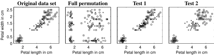
Original data set Full permutation Test 1 Test 2

2 4 6

0 0.5 1 1.5 2 2.5

Petal length in cm

Petal width in cm

2 4 6

0 0.5 1 1.5 2 2.5

Petal length in cm

2 4 6

0 0.5 1 1.5 2 2.5

Petal length in cm

2 4 6

0 0.5 1 1.5 2 2.5

Petal length in cm

Figure 2: Scatter plots of original Iris data set and randomized versions for full permutation of the data and for Tests 1 and 2 (one sample for each test). The data points belong to three different classes denoted by different markers, and they are scattered against petal length and width in centimeters.

the other hand, this observation can lead us to find a classifier that can exploit the possibly existing dependency and thus improve the classification accuracy further, as discussed in the introduction.

There are three important properties of the permutation-based p-values and the two tests pro-posed here. The first one is that the number of missing values, that is, the number of entries in D that are empty because they do not have measured values, will be distributed equally across columns in the original data set D and the randomized data sets D′; this is necessary for a fair p-value compu-tation. The second property is that the proposed permutations are always relevant regardless of the data domain, that is, values are permuted always within the same column, which does not change the domain of the randomized data sets. Finally, we have that unbalanced data sets, that is, data sets where the distribution of class labels is not uniform, remain equally unbalanced in the randomized samples.

In all, with permutation tests we obtain useful statistics about the classification result. No test is better than the other, but all provide us with information about the classifier. Each p-value is a statistic about the classifier performance; each p-value depends on the original data (whether it contains some real structure or not) and the classifier (whether it is able to use certain structure in the data or not).

In Figure 2, we give as an example one randomization for each test on the well-known Iris data set. We show here the projection of two features, before and after randomizations according to each one of the tests. For comparison, we include a test corresponding to full permutation of the data where each column is permuted separately, breaking the connection between the features and mixing the values between different classes. Note how well Test 2 has preserved the class structure compared to other tests. To provide more intuitions, in this case a very simple classifier, which predicts the class by means of one single of these two features would suffice in reaching a very good accuracy. In other words, the dependency between the two features is not significant as such, so that a more complex classifier making use of such dependency would end up having a high

p-value with Test 2. We will discuss the Iris data more in the experiments.

3.2 Handling Instability of the Error

return different error estimates e(f,D) if, for example, 10-fold cross-validation is used. So the question is, how can we ensure that the p-values given by the tests are stable to such variance?

The empirical p-value depends heavily on the correct estimation of the original classification accuracy, whereas the good estimation of the classification errors of the randomized data sets is not so important. However, exactly the same classification procedure has to be used for both the original and randomized data for the p-value to be valid. Therefore, we propose the following solution to alleviate the problem of having instable test statistic: We train the classifier on the original data r times, thus obtaining r different error estimates E=_{e1(f,D), . . . ,er(f,D)}on D. Next, we obtain k randomized samples of D according to the desired null hypothesis and compute the p-value for

each one of those original errors e_∈E. We obtain therefore r different p-values by using the same k randomized data sets for each computation. We finally output the average of those r different p-values as the final empirical p-value.

Note that in total we will compute the error of the classifier r+k times: r times on the original

data and one time for each of the k randomized data sets. Of course, the larger the k and the larger the r, the more stable the final averaged p-value would be. A larger r decreases the variance in the final p-value due to the estimation of the classification error of the original data set whereas a larger

k decreases the variance in the final p-value due to the random sampling from the null distribution.

In practice, we have observed that a value of r=10 and k=100 produce sufficiently stable results. This solution is closely related to calculating the statistic ρ, or calculating the test statistic U of the Wilcoxon-Mann-Whitney two-sample rank-sum test (Good, 2000). However, it is not valid to apply these approaches in our context as the r classification errors of the original data are not independent of each other. Nevertheless, the proposed solution has the same good properties as the

ρand U statistics as well as it generalizes the concept of empirical p-value to instable results. A different solution would be to use a more accurate error estimate. For example, we could use leave-one-out cross-validation or cross-validation with 100 folds instead of 10-fold cross-validation. This will decrease the variability but increase the computation time dramatically as we need to perform the same slow classification procedure to all k randomized samples as well. However, it turns out that the stability issue is not vital for the final result; our solution produces sufficiently stable p-values in practice.

3.3 Example

We illustrate the concept of the tests by studying the small artificial example presented in the intro-duction in Figure 1. Consider the two data sets D1and D2 given in Figure 1. The first data set D1

was generated as follows: in the first eight rows corresponding to class+, each element is indepen-dently sampled to bexwith probability 80% andootherwise; in the last eight rows the probabilities are the other way around. Note that in the data set D1the features are independent given the class

since, for example, knowing that Xj1

i =x inside class +does not increase the probability of X j2

i

being x. The data set D2was generated as follows: the first four rows contain x, the second four

rows containo, the third four rows containxin the first four columns andoin the last four columns, and the last four rows containoin the first four columns andxin the last four columns; finally, 10% of noise was added to the data set, that is, eachxwas flipped toowith probability of 10%, and vice versa.

Observe that both D1and D2have a clear separation into the two given classes,+and–.

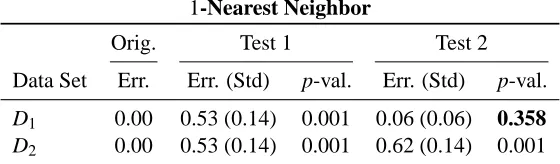
1-Nearest Neighbor

Orig. Test 1 Test 2

Data Set Err. Err. (Std) p-val. Err. (Std) p-val.

D1 0.00 0.53 (0.14) 0.001 0.06 (0.06) 0.358

D2 0.00 0.53 (0.14) 0.001 0.62 (0.14) 0.001

Table 1: Average error and p-value for Test 1 and Test 2 when using the 1-Nearest Neighbor classi-fier to data sets of Figure 1.

purposes, we analyze this with the 1-Nearest Neighbor classifier using the leave-one-out cross-validation given in Equation (1). Results for Test 1 and Test 2 are summarized in Table 1. The classification error obtained in the original data is 0.00 for both D1and D2, which is expected since

the data sets were generated to contain clear class structure.

First, we use the standard permutation test (i.e., permuting labels, Test 1) to understand the behavior under the null hypothesis where data points and labels are independent. We produce 1000 random permutations of the class labels for both the data sets D1 and D2, and perform the same

leave-one-out cross-validation procedure to obtain a classification error for each randomized data set. On the randomized samples of data set D1 we obtain an average classification error of 0.53,

a standard deviation 0.14 and a minimum classification error of 0.13. For the randomized data from D2 the corresponding values are 0.53, 0.14 and 0.19, respectively. These values result in

two empirical p-values of both 0.001 on both the data sets D1 and D2. Thus, we can say that the

classifiers are significant under the null hypothesis that data and labels are independent. That is, the connection between the data and the class labels is real in both data sets and the 1-Nearest Neighbor classifier is able to find that connection in both data sets, resulting into a good classification accuracy. However, it is easy to argue that the results of Test 1 do not provide much information about the classifier performance. Actually the main problem of Test 1 is that p-values tend to be always very low as the null hypothesis is typically easy to reject. To get more information of the properties of the classifiers, we study next the performance of the classifiers by taking into account the inner structure of data sets D1and D2by applying Test 2. Again, we produce 1000 random samples of the

data sets D1and D2by permuting each column separately inside each class. The same leave-one-out

cross-validation procedure is performed for the randomized samples, obtaining for the data set D1

the average classification error of 0.06, standard deviation of 0.06 and a minimum value of 0.00. For the data set D2the corresponding values are 0.62, 0.14 and 0.19, respectively. Therefore, under

Test 2 the empirical p-values are 0.358 for the data set D1and 0.001 for the data set D2.

We can say that, for Test 2, the 1-Nearest Neighbor classifier is significant for data set D2but

not for data set D1. Indeed, the data set D1 was generated so that the features are independent

inside the classes, and hence, the good classification accuracy of the algorithm on D1is simply due

to different value distributions across the classes. Note, however, that none of the features in the data set D1 is sufficient alone to correctly classify all the samples due to the noise in the data set.

Thus using a combination of multiple features for classification is necessary for obtaining a good accuracy, even though the features are independent of each other. For data set D2we have that the

4. Analysis

In this section we analyze the properties of the tests and demonstrate the behavior of the different p-values on simulated data. First, we state the relationships between the different sets of permutations.

4.1 Connection between Test 1 and Test 2

Remember that the random samples from Test 1 are obtained by permuting the class labels and the samples from Test 2 by permuting the features inside each class. To establish a connection between these randomizations, we study the randomization where each data column is permuted separately, regardless of the class label. This corresponds to the full permutation presented in Figure 2 in Section 3.1 for Iris data set. It breaks the connection between the features, and furthermore, between the data and the class labels. The following result states the relationship between Test 1, Test 2 and the full permutation method.

Proposition 2 LetΠl(D),Πc(D),Πcc(D)be the sets of all possible randomized data sets obtained from D via permuting labels (Test 1), permuting data columns (full permutation), or permuting data columns inside class (Test 2), respectively. The following holds,

(1) Πl(D)_⊂Πc(D)

(2) Πcc(D)_⊂Πc(D) (3) Πl(D)₆=Πcc(D)

Note that Πl(D), Πc(D) andΠcc(D) refer to sets of data matrices. Therefore, we have that permuting the data columns is the randomization method producing the most diverse samples, while permuting labels (Test 1) and permuting data within class (Test 2) produce different randomized samples.

Actually, the relationship stated by Proposition 2 implies the following property: the p-value obtained by permuting the data columns is typically smaller than both the p-values obtained from Test 1 and Test 2. The reason is that all the randomized data sets obtained by Test 1 and Test 2 can also be obtained by permuting data columns and the additional randomized data sets obtained by permuting the columns are, in general, even more random. Theoretically, permuting the data columns is a combination of Test 1 and Test 2, and thus, it is not a useful test. In practice, we have observed that the p-value returned by permuting the data columns is very close to the p-value of Test 1, which tends to be much smaller than the p-value of Test 2.

Considering Proposition 2, it makes only sense to restrict the randomization to classes by using Test 2, whenever Test 1 has produced a small p-value. That is, it is only reasonable to study whether the classifier uses feature dependency in separating the classes if it has found a real class structure.

4.2 Behavior of the Tests

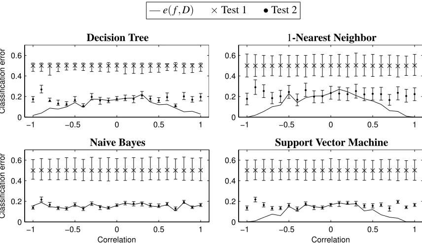
— e(f,D) _×Test 1 _•Test 2

Decision Tree 1-Nearest Neighbor

−1 −0.5 0 0.5 1

0 0.2 0.4 0.6

Classification error

−1 −0.5 0 0.5 1

0 0.2 0.4 0.6

Naive Bayes Support Vector Machine

−1 −0.5 0 0.5 1

0 0.2 0.4 0.6

Classification error

Correlation

−1 −0.5 0 0.5 1

0 0.2 0.4 0.6

Correlation

Figure 3: Average values of stratified 10-fold cross-validation error (y-axis) for varying values of correlation between the features per class (x-axis). The solid line shows the error on the original data, and symbols_×and_•represent the average of the error on 1000 randomized samples obtained from Test 1 and from Test 2, respectively. Each average of the error on the randomized samples_× and_•is depicted together with the[1%,99%]-deviation bar. If the solid line falls below the bars the null hypothesis associated to the test is rejected; if the solid line crosses inside or above the bars the null hypothesis cannot be rejected with significance levelα=0.01.

covariance ρ. The first 100 samples are assigned with class label y= +1 with probability 1₋t

and y=₋1 with probability t. For the other 100 samples the probabilities are the opposite. The probability t _∈[0,0.5]represents the noise level. When t=0.5, there is no class structure at all. Note that the correlation between the features improves the class separation: if the correlationρ=1 and the noise t =0, we have that the class y=x1−x2 where x1, x2 are the values of the first and

second features, respectively.

For these data sets (with varying parameters of noise and correlation) we use as an error estimate the stratified 10-fold cross-validation error. We study the behavior of four classifiers: 1-Nearest Neighbor, Decision Tree, Naive Bayes and Support Vector Machine. We use Weka 3.6 data mining software (Witten and Frank, 2005) with the default parameters of the implementations of those classification algorithms. The Decision Tree classifier is similar to C4.5 algorithm, and the default kernel used with Support Vector Machine is linear. Tuning the parameters of these algorithms is not in the scope of this paper; our objective is to show the behavior of the discussed p-values for some selected classifiers.

Correlation 0.0 Correlation 0.5 Correlation 0.8 Correlation 1.0

0 0.1 0.2 0.3 0.4 0.5 0

0.2 0.4 0.6

Classification error

Noise

0 0.1 0.2 0.3 0.4 0.5 0

0.2 0.4 0.6

Noise

0 0.1 0.2 0.3 0.4 0.5 0

0.2 0.4 0.6

Noise

0 0.1 0.2 0.3 0.4 0.5 0

0.2 0.4 0.6

Noise

Figure 4: Average values of stratified 10-fold cross-validation error (y-axis) for the Decision Tree classifier when noise varies on the original data set (x-axis) with four fixed correlation values be-tween the features inside the classes. The solid line shows the error on the original data, and sym-bols_×and_•show the average error on 1000 randomized samples from Test 1 and Test 2, respec-tively. Each average of the error on the randomized samples_×and_•is depicted together with the

[1%,99%]-deviation bar below which the associated null hypothesis is rejected with significance levelα=0.01.

data. The symbols “_×” and “_•” represent the average error obtained by the classifier on 1000 randomized samples from Test 1 and Test 2, respectively. When the solid line of e(f,D) falls below the[1%,99%]-deviation bars, the corresponding associated null hypothesis is rejected with significance level α=0.01. Actually, the correspondence between the confidence intervals and hypotheses testing is only approximately true since the definition of empirical p-value contains the addition of 1 in both the numerator and denominator. However, the practical difference is negligible.

First, note that the Decision Tree, 1-Nearest Neighbor and Support Vector Machine classifiers have been able to exploit the dependency between the features, that is, the classification error goes to zero when there is either a high positive or negative correlation between the features. However, with Naive Bayes classifier the classification error seems to be independent of the correlation between the features.

For all classifiers we observe that the null hypothesis associated to Test 1 (i.e., labels and data are independent) is always rejected. Thus the data contains a clear class structure as expected since there exists no class noise in the data. All classifiers are therefore significant under Test 1.

Another expected observation is that the null hypothesis for Test 2 (i.e., features are independent within class) tends to be rejected as the magnitude of the correlation between features increases. That is, the correlation is useful in classifying the data. When the magnitude of the correlation is larger than approximately 0.4, the Decision Tree, Nearest Neighbor and Support Vector Machine classifiers reject the null hypothesis. Thus these classifiers produce significant results under Test 2 when the features are highly correlated.

Finally, Figure 4 shows the behavior of the Decision Tree classifier when the noise t∈[0,0.5]is increased on the x-axis. We also vary the correlationρbetween the features per class and show the results on four cases: zero correlation, 0.5, 0.8 and total correlation. We observe that as the noise increases the p-values tend to be larger. Therefore, it is more difficult to reject the null hypothesis on very noisy data sets, that is, when the class structure is weak. This is true for both Test 1 and Test 2. However, Test 1 rejects the null hypothesis even if there is 30% of noise. This supports the fact already observed in related literature (Golland et al., 2005), that even a weak class structure is easily regarded as significant with Test 1. Compared to this, Test 2 gives more conservative results.

4.3 Power Analysis of Test 2

The power of a statistical test is the probability that the test will reject the null hypothesis when the alternative hypothesis is true. The power of the test depends on how much or how clearly the null hypothesis is false. For example, in our case with Test 2, a classifier may rely solely on a strong dependency structure between some specific features in the classification, or it may use a weak feature dependency to slightly improve the classification accuracy. Rejecting the null hypothesis of Test 2 is much easier in the former than in the latter case. Note, however, that a strong dependency between the features is not always useful in separating the classes, as seen in Figure 2 with Iris data set. So, the question with Test 2 is whether the classifier is exploiting some of the dependency structure between the features in the data and how important such feature dependency is for the classification of the data.

In general, the power of the test can only be analyzed in special cases. Nevertheless, such analysis can give some general idea of the power the test. Next, we present a formal power analysis in the particular case where we vary the correlation between the features that is useful in separating the classes from each other. Note, however, that there exist also other types of dependency than correlation. The amount of correlation is just easy to measure, thus being suitable for formal power analysis.

We present the power analysis on similar data as studied in Section 4.2. The results in the previous subsection can be seen as informal power analysis. In summary, we observed that when the magnitude of the correlation in the data studied in Section 4.2 was larger than about 0.5 and the classifier was exploiting the feature dependency, that is, a classifier different from Naive Bayes, Test 2 was able to reject the null hypothesis. However, based on the data it is clear that even smaller correlations increased the class separation and were helpful in classifying the data but Test 2 could not regard such improvement as significant. The following analysis supports these observations.

Let the data set X consist of n points with two features belonging to two classes, +1 and₋1. Let a point x_∈X be in class y= +1 with probability 0.5 and in class y=₋1 with probability 0.5. Let the point x∈X be sampled from two-dimensional normal distribution with mean(0,0), unit variances and covariance yρwhereρ_∈[0,1]is a given parameter. Thus, in the first class, y= +1, the correlation between the two features is positive and in the second class, y=₋1, it is negative. Compared to the data sets in Section 4.2, now the covariance changes between the classes, not the mean vector. An optimal classifier assigns a point x_∈X to class y= +1 if x1x2>0 and to class

y=₋1 if x1x2<0, where xiis the i-th feature of the vector x.

the signum function. If the classifier is not optimal, it will just decrease the power of the test. The nonoptimality of the classifier could be taken into account by introducing a probability t for reporting a nonoptimal class label; this approach is used in the next subsection for power analysis of Test 1 but is left out here for simplicity in the analysis. Under this optimality scenario, the probability of correctly classifying a sample is

Pr(sgn(x1x2) =y) =1

2Pr(x1x2>0|y= +1) + 1

2Pr(x1x2<0|y=−1)

=Pr(x1x2>0_|y= +1) =2

Z _∞

0 Z _∞

0

Pr(x1,x2)dx1dx2 =2 Z _∞ 0 Z _∞ 0 1

2πp1₋ρ2exp

−x

2

1−2ρx1x2+x22

2(1₋ρ2₎

dx1dx2

=1

2+ 1

πarcsinρ, (2)

where Pr(x1,x2)is just the standardized bivariate normal distribution. The null hypothesis

corre-sponds to the case where the correlation parameter is zero, ρ=0, that is, no feature dependency exists. In that case, the probability of correctly classifying a sample is 1/2.

In our randomization approach, we are using classification error as the test statistic. Since we assume that the optimal classifier is given, we use all the n points of the data set X for testing the classifier and calculating the classification error. Under the null hypothesis H0 and under the

alternative hypothesis H1 of Test 2, the classification errors e(f |H0) and e(f |H1)are distributed

as follows:

n_·e(f _|H0)∼Bin

n,1

2

≈

N

2,

n

4

,

n_·e(f _|H1)∼Bin

n,1

2− 1

πarcsinρ

≈

N

2−

n

πarcsinρ, n

4−

n π2arcsin

2_ρ,

where 1_2−π1arcsinρis the probability of incorrectly classifying a sample by Equation (2). The nor-mal approximation

N

2− 1

πarcsinρ)>5. This holds, for example, if n_≥20 andρ_≤0.7.

Now the power of Test 2 for this generated data is the probability of rejecting the null hypothesis

H0 of ρ=0 with significance levelα when the alternative hypothesis H1 is that the correlation ρ>0. Note that we are implicitly assuming that the classifier is optimal, that is, we are excluding the classifier quality from the power analysis. Thus, the power is the probability that e(f _|H1)is smaller than 1₋αof the errors e(f_|H0)under the alternative hypothesis H1:

Power=Pr

e(f _|H1)<F_e−₍1_f|H0)(α)

≈Pr 1

2− 1

πarcsinρ+

r 1 4n−

1

nπ2arcsin 2_ρ

·Z<1

2+ 1 2√nΦ

−1_(α)

!

=Φ



2√n arcsin_q ρ+πΦ−1(α)

π2_{−4 arcsin}2_ρ



0.1 0.3

0.5

0.7

0.9

Number of rows

Correlation

101 102 103 104

0 0.2 0.4 0.6 0.8 1

(a)α=0.05

0.1

0.3 0.50.7

0.9

Number of rows

Correlation

101 102 103 104

0 0.2 0.4 0.6 0.8 1

(b)α=0.01

Figure 5: Contour plots of the statistical power of Test 2 as a function of the number of rows n in the generated data set and the correlation parameterρ. Each solid line corresponds to a constant value of the power that is given on top of the contour. The power values are calculated by Equation (3) for two different values of significance levelα.

where Fe(f|H0)is the cumulative distribution function of e(f|H0), Z is a random variable following standard normal distribution andΦ is the cumulative distribution function of the standard normal distribution. Note that we are using exact p-value instead of empirical p-value, effectively leaving out the influence of variance by using k randomized samples; see Fay et al. (2007) for analysis of resampling risk of using k samples. However, this has little effect to the power of the test. When the correlationρ=0, the power isα, that is, when the null hypothesis is true, it is rejected incorrectly aboutαof the times. Therefore,αis really the significance level of the tests.

In Figure 5 we present contour plots of the statistical power in Equation (3) for different values of the two varying parameters. As expected, the higher the correlationρand the number of rows

n are, the higher the statistical power of Test 2 is. For example, if the data set contains about 1000

rows, we can infer with 90% probability that the classifier is exploiting the feature dependency of approximately a correlation of 0.2 in the data. The results are also in line with the results from Section 4.2 although the studied data sets are slightly different. When the significance level used is

α=0.01 we can infer that the classifier is exploiting the feature dependency of correlation larger than 0.4 approximately 90% of the times when the data set has 200 rows.

4.4 Power Analysis of Test 1

Let the data set X consist of n observations belonging to two different classes with equal probability. We assume that we have a classifier f whose error rate is t_∈[0,1], that is, the classifier assigns each observation to the correct class with probability 1₋t. Another way to see this is that the classifier f is optimal but the original class label of each point is erroneous with probability t. We perform

power analysis of Test 1 for this general form of data.

Note that the results in Section 4.2 can be seen as informal power analysis of Test 1 on similar setting as studied here. The results in Figure 4 can be summarized as follows. When the error rate was smaller than t<0.4, Test 1 was able to reject the null hypotheses. Note, however, that the error rate t used in this section is not directly comparable to the error rate used in Section 4.2.

The power analysis of Test 1 proceeds similarly as in the previous subsection for Test 2. Under the null hypothesis H0 and under the alternative hypothesis H1 of Test 1, the classification errors e(f _|H0)and e(f _|H1)are distributed as follows:

n_·e(f _|H0)_∼Bin

n,1

2

≈

N

2,

n

4

,

n_·e(f _|H1)_∼Bin(n,t)_≈

N

The null hypothesis H0 assumes that there is no connection between the data and the class labels

thus the probability of incorrect classification is 1/2 as the classes are equally probable. Note that the null hypothesis corresponds to the case where the error rate of the classifier f is t=1/2.

Now the power of Test 1 is the probability of rejecting the null hypothesis H0with significance

levelαwhen the alternative hypothesis H1is true, that is,

Power=Pre(f _|H1)<F_e−₍1_f|H0)(α)

≈Pr t+

r

t(1₋t)

n Z<

1 2+

1 2√nΦ

−1_(α)

!

=Φ (1−2t)

√

n+Φ−1_(α)

2pt(1₋t)

!

, (4)

where the same notation as in the previous subsection is used. First, note that when the null hypoth-esis is true, that is, t=1/2, the power of Test 1 calculated by Equation (4) equals the significance levelαas it should.

In Figure 6 we present contour plots of the statistical power of Test 1 calculated by Equation (4) for different values of parameters. As expected, when the number of observations n increases or the error rate t decreases, the power increases. Furthermore, the larger the significance levelαis, the larger the power of Test 1 is. When the parameter values areα=0.01, n=200 and t=0.4, the power of Test 1 is about 0.7 that is comparable to the results in Section 4.2.

0.1

0.3 0.5

0.7 0.9

Number of rows

Probability of misclassification

101 102 103 104

0 0.1 0.2 0.3 0.4 0.5

(a)α=0.05

0.1

0.3 0.5

0.7 0.9

Number of rows

Probability of misclassification

101 102 103 104

0 0.1 0.2 0.3 0.4 0.5

(b)α=0.01

Figure 6: Contour plots of the statistical power of Test 1 as a function of the number of rows n in the generated data set and the probability of misclassification t. Each solid line corresponds to a constant value of the power that is given on top of the contour. The power values are calculated by Equation (4) for two different values of significance levelα.

5. Empirical Results

In this section, we give extensive empirical results on 33 various real data sets from UCI machine learning repository (Asuncion and Newman, 2007). Basic characteristics of the data sets are de-scribed in Table 2. The data sets are divided into three categories based on their size: small, medium and large. Some data sets contain only nominal or numeric features whereas some data sets contain both kind of features (mixed). About one-third of the data sets contain also missing values. Notice that in most data sets the features are measured in different scales, thus it is not sensible to swap the values between different features. This justifies why it is only reasonable to consider column-wise permutations, and why some recent data mining randomization methods (Gionis et al., 2007; Ojala et al., 2009; Chen et al., 2005) are not generally applicable in assessing classification results.

In the experiments we use Weka 3.6 data mining software (Witten and Frank, 2005) that contains open source Java implementations of many classification algorithms. We use four different types of classification algorithms with the default parameters: Decision Tree, Naive Bayes, 1-Nearest Neighbor and Support Vector Machine classifier. The Decision Tree classifier is similar to C4.5 algorithm. The default kernel used with Support Vector Machine is linear. Missing values and the combination of nominal and numerical values are given as such as the input for the classifiers; the default approaches in Weka of the classifiers are used to handle these cases. Notice that tuning the parameters of these algorithms is not in the scope of this paper; our objective is to show the behavior of the discussed p-values for some selected classifiers on various data sets.

Data Set Rows Features Classes Missing Domain

S

ma

ll

Audiology 226 70 24 2.0% nominal

Autos 205 25 6 1.2% mixed

Breast 286 9 2 0.3% nominal

Glass 214 9 6 No numeric

Hepatitis 155 19 2 5.7% mixed

Ionosphere 351 34 2 No numeric

Iris 150 4 3 No numeric

Lymph 148 18 4 No mixed

Promoters 106 57 2 No nominal

Segment 210 19 7 No numeric

Sonar 208 60 2 No numeric

Spect 267 22 2 No nominal

Tumor 339 17 21 3.9% nominal

Votes 435 16 2 5.6% nominal

Zoo 101 17 7 No mixed

M

ed

iu

m

Abalone 4177 8 28 No mixed

Anneal 898 38 5 65.0% mixed

Balance 625 4 3 No numeric

Car 1728 6 4 No nominal

German 1000 20 2 No mixed

Mushroom 8124 22 2 1.4% nominal

Musk 6598 166 2 No numeric

Pima 768 8 2 No numeric

Satellite 6435 36 6 No numeric

Spam 4601 57 2 No numeric

Splice 3190 60 3 No nominal

Tic-tac-toe 958 9 2 No nominal

Yeast 1484 8 10 No numeric

L

ar

g

e

Adult 48842 15 2 0.9% mixed

Chess 28056 6 18 No mixed

Connect-4 67557 42 3 No nominal

Letter 20000 16 26 No numeric

Shuttle 58000 9 7 No numeric

set into training set with 10 000 random rows and to test set with the rest of the rows. We use 100 randomized data sets for calculating the empirical p-values with large data sets. The reason for the smaller number of randomized samples for medium and large data sets is mainly computation time. However, 100 samples is usually enough for statistical inference. Furthermore, as seen in Section 4 the power of the tests is greater when the data sets have more rows, that is, with large data sets it is easier to reject the null-hypotheses, supporting the need of fewer randomized samples in hypothesis testing.

Since the original classification error is not a stable result due to the randomness in training the classifier and dividing the data set into test and train data, we perform the same classification procedure ten times for the original data sets and calculate an empirical p-value for each of the ten results. This was described in Section 3.2. We give the average value of these empirical p-values as well as the average value and the standard deviation of the original classification errors.

As we are testing multiple hypotheses simultaneously, we need to correct for multiple compar-isons. We apply the approach by Benjamini and Hochberg (1995) to control the false discovery rate (FDR), that is, the expected proportion of results incorrectly regarded as significant. In the exper-iments, we restrict the false discovery rate belowα=0.05 separately for Test 1 and Test 2. In the Benjamini-Hochberg approach, if p1, . . . ,pmare the original empirical p-values in increasing order,

the results p1, . . . ,pl are regarded as significant where l is the largest value such that pl ≤_mlα.

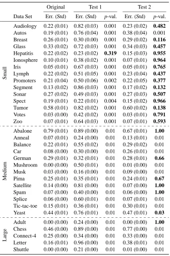
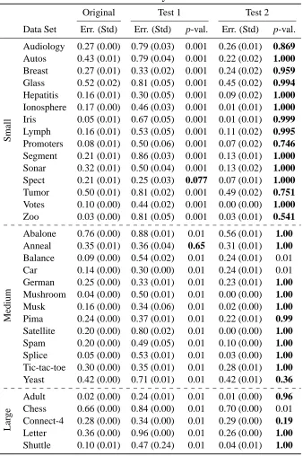
The significance testing results for the Decision Tree classifier are given in Table 3, for Naive Bayes in Table 4, for 1-Nearest Neighbor classifier in Table 5 and finally for Support Vector Ma-chine classifier in Table 6. The mean and the standard deviation of the 10 original classification errors are given as well as the mean and standard deviation of the errors on the 1000 or 100 ran-domized samples with Test 1 and Test 2. The empirical p-values corresponding to nonsignificant results, when the false discovery rate is restricted below 0.05, are in boldface in the tables. With all classifiers, the largest significant empirical p-value was 0.01. The smallest non-significant p-values were 0.03 with Decision Tree and 1-Nearest Neighbor classifiers, 0.08 with Naive Bayes classifier and 0.19 with Support Vector Machine classifier.

The results for the traditional permutation method Test 1 show that the classification errors with most data sets are regarded as significant. These results show that the data sets contain clear class structure. However, they do not give any additional insight for understanding the class structure in the data sets.

There are two reasons why the simple permutation test, Test 1, regards the class structure of the data sets as significant. Firstly, most of the data sets that are publicly available, as all the data sets used in this paper, have already passed some quality checks, that is, someone has already found some interesting structure in them. Secondly, and as a more important reason, the traditional permutation tests easily regard the results as significant even if there is only a slight class structure present because in the corresponding permuted data sets there is no class structure, especially if the original data set is large.

Furthermore, the few results which were regarded as nonsignificant with Test 1 are with such classifiers that have not performed well on the data. That is, the other classifiers have produced smaller classification errors on the same data sets, and, in contrast, these results are regarded as significant.

Decision Tree

Original Test 1 Test 2

Data Set Err. (Std) Err. (Std) p-val. Err. (Std) p-val.

S

ma

ll

Audiology 0.22 (0.01) 0.82 (0.03) 0.001 0.23 (0.02) 0.482

Autos 0.19 (0.01) 0.76 (0.04) 0.001 0.38 (0.04) 0.001 Breast 0.26 (0.01) 0.30 (0.00) 0.001 0.29 (0.02) 0.116

Glass 0.33 (0.02) 0.72 (0.03) 0.001 0.34 (0.03) 0.457

Hepatitis 0.22 (0.02) 0.23 (0.02) 0.319 0.15 (0.03) 0.955

Ionosphere 0.10 (0.01) 0.38 (0.02) 0.001 0.07 (0.01) 0.964

Iris 0.05 (0.01) 0.67 (0.03) 0.001 0.05 (0.01) 0.765

Lymph 0.22 (0.02) 0.51 (0.05) 0.001 0.23 (0.04) 0.437

Promoters 0.21 (0.04) 0.50 (0.06) 0.002 0.22 (0.05) 0.377

Segment 0.13 (0.02) 0.86 (0.03) 0.001 0.17 (0.02) 0.132

Sonar 0.27 (0.02) 0.49 (0.03) 0.001 0.27 (0.03) 0.507

Spect 0.19 (0.01) 0.22 (0.01) 0.004 0.15 (0.02) 0.966

Tumor 0.58 (0.01) 0.82 (0.02) 0.001 0.60 (0.02) 0.138

Votes 0.03 (0.00) 0.42 (0.02) 0.001 0.03 (0.01) 0.791

Zoo 0.07 (0.01) 0.64 (0.03) 0.001 0.07 (0.01) 0.593

M

ed

iu

m

Abalone 0.79 (0.01) 0.89 (0.00) 0.01 0.67 (0.01) 1.00

Anneal 0.07 (0.01) 0.24 (0.00) 0.01 0.13 (0.01) 0.01 Balance 0.22 (0.01) 0.55 (0.02) 0.01 0.29 (0.02) 0.01

Car 0.08 (0.00) 0.30 (0.00) 0.01 0.26 (0.01) 0.01

German 0.29 (0.01) 0.32 (0.01) 0.01 0.28 (0.01) 0.66

Mushroom 0.00 (0.00) 0.50 (0.01) 0.01 0.01 (0.00) 0.01 Musk 0.03 (0.00) 0.16 (0.00) 0.01 0.09 (0.00) 0.01 Pima 0.25 (0.01) 0.35 (0.01) 0.01 0.24 (0.01) 0.67

Satellite 0.14 (0.00) 0.81 (0.00) 0.01 0.07 (0.00) 1.00

Spam 0.07 (0.00) 0.40 (0.00) 0.01 0.06 (0.00) 1.00

Splice 0.06 (0.00) 0.60 (0.01) 0.01 0.07 (0.01) 0.01 Tic-tac-toe 0.15 (0.01) 0.36 (0.01) 0.01 0.30 (0.01) 0.01 Yeast 0.44 (0.01) 0.76 (0.01) 0.01 0.47 (0.01) 0.03

L

ar

g

e

Adult 0.00 (0.00) 0.24 (0.00) 0.01 0.00 (0.00) 1.00

Chess 0.46 (0.00) 0.89 (0.00) 0.01 0.77 (0.00) 0.01 Connect-4 0.25 (0.00) 0.34 (0.00) 0.01 0.33 (0.00) 0.01 Letter 0.16 (0.01) 0.96 (0.00) 0.01 0.38 (0.01) 0.01 Shuttle 0.00 (0.00) 0.21 (0.00) 0.01 0.01 (0.00) 0.01

Naive Bayes

Original Test 1 Test 2

Data Set Err. (Std) Err. (Std) p-val. Err. (Std) p-val.

S

ma

ll

Audiology 0.27 (0.00) 0.79 (0.03) 0.001 0.26 (0.01) 0.869

Autos 0.43 (0.01) 0.79 (0.04) 0.001 0.22 (0.02) 1.000

Breast 0.27 (0.01) 0.33 (0.02) 0.001 0.24 (0.02) 0.959

Glass 0.52 (0.02) 0.81 (0.05) 0.001 0.45 (0.02) 0.994

Hepatitis 0.16 (0.01) 0.30 (0.05) 0.001 0.09 (0.02) 1.000

Ionosphere 0.17 (0.00) 0.46 (0.03) 0.001 0.01 (0.01) 1.000

Iris 0.05 (0.01) 0.67 (0.05) 0.001 0.01 (0.01) 0.999

Lymph 0.16 (0.01) 0.53 (0.05) 0.001 0.11 (0.02) 0.995

Promoters 0.08 (0.01) 0.50 (0.06) 0.001 0.07 (0.02) 0.746

Segment 0.21 (0.01) 0.86 (0.03) 0.001 0.13 (0.01) 1.000

Sonar 0.32 (0.01) 0.50 (0.04) 0.001 0.13 (0.02) 1.000

Spect 0.21 (0.01) 0.25 (0.03) 0.077 0.07 (0.01) 1.000

Tumor 0.50 (0.01) 0.81 (0.02) 0.001 0.49 (0.02) 0.751

Votes 0.10 (0.00) 0.44 (0.02) 0.001 0.00 (0.00) 1.000

Zoo 0.03 (0.00) 0.81 (0.05) 0.001 0.03 (0.01) 0.541

M

ed

iu

m

Abalone 0.76 (0.00) 0.88 (0.01) 0.01 0.56 (0.01) 1.00

Anneal 0.35 (0.01) 0.36 (0.04) 0.65 0.31 (0.01) 1.00

Balance 0.09 (0.00) 0.54 (0.02) 0.01 0.24 (0.01) 0.01

Car 0.14 (0.00) 0.30 (0.00) 0.01 0.24 (0.01) 0.01

German 0.25 (0.00) 0.33 (0.01) 0.01 0.23 (0.01) 1.00

Mushroom 0.04 (0.00) 0.50 (0.01) 0.01 0.00 (0.00) 1.00

Musk 0.16 (0.00) 0.34 (0.06) 0.01 0.02 (0.00) 1.00

Pima 0.24 (0.00) 0.37 (0.01) 0.01 0.22 (0.01) 0.99

Satellite 0.20 (0.00) 0.80 (0.02) 0.01 0.00 (0.00) 1.00

Spam 0.20 (0.00) 0.49 (0.05) 0.01 0.10 (0.00) 1.00

Splice 0.05 (0.00) 0.53 (0.01) 0.01 0.03 (0.00) 1.00

Tic-tac-toe 0.30 (0.00) 0.35 (0.01) 0.01 0.28 (0.01) 1.00

Yeast 0.42 (0.00) 0.71 (0.01) 0.01 0.42 (0.01) 0.36

L

ar

g

e

Adult 0.02 (0.00) 0.24 (0.01) 0.01 0.01 (0.00) 0.96

Chess 0.66 (0.00) 0.84 (0.00) 0.01 0.70 (0.00) 0.01 Connect-4 0.28 (0.00) 0.34 (0.00) 0.01 0.29 (0.00) 0.19

Letter 0.36 (0.00) 0.96 (0.00) 0.01 0.26 (0.00) 1.00

Shuttle 0.10 (0.01) 0.47 (0.24) 0.01 0.04 (0.01) 1.00

1-Nearest Neighbor

Original Test 1 Test 2

Data Set Err. (Std) Err. (Std) p-val. Err. (Std) p-val.

S

ma

ll

Audiology 0.26 (0.01) 0.86 (0.03) 0.001 0.32 (0.03) 0.030

Autos 0.26 (0.01) 0.77 (0.03) 0.001 0.45 (0.03) 0.001 Breast 0.31 (0.02) 0.41 (0.03) 0.007 0.32 (0.03) 0.324

Glass 0.30 (0.01) 0.74 (0.04) 0.001 0.42 (0.03) 0.001 Hepatitis 0.19 (0.01) 0.33 (0.04) 0.002 0.14 (0.03) 0.970

Ionosphere 0.13 (0.00) 0.46 (0.03) 0.001 0.26 (0.01) 0.001 Iris 0.05 (0.00) 0.66 (0.05) 0.001 0.02 (0.01) 0.962

Lymph 0.18 (0.02) 0.53 (0.04) 0.001 0.20 (0.03) 0.307

Promoters 0.19 (0.02) 0.50 (0.06) 0.001 0.26 (0.04) 0.083

Segment 0.14 (0.01) 0.86 (0.03) 0.001 0.15 (0.02) 0.266

Sonar 0.13 (0.01) 0.50 (0.04) 0.001 0.27 (0.03) 0.001 Spect 0.24 (0.02) 0.32 (0.04) 0.011 0.18 (0.02) 0.970

Tumor 0.66 (0.02) 0.88 (0.02) 0.001 0.62 (0.02) 0.860

Votes 0.08 (0.01) 0.47 (0.03) 0.001 0.01 (0.00) 1.000

Zoo 0.03 (0.01) 0.75 (0.05) 0.001 0.04 (0.02) 0.333

M

ed

iu

m

Abalone 0.80 (0.00) 0.90 (0.00) 0.01 0.68 (0.01) 1.00

Anneal 0.05 (0.00) 0.40 (0.02) 0.01 0.08 (0.01) 0.01 Balance 0.20 (0.01) 0.57 (0.02) 0.01 0.35 (0.02) 0.01

Car 0.22 (0.01) 0.41 (0.05) 0.01 0.29 (0.01) 0.01

German 0.28 (0.01) 0.42 (0.02) 0.01 0.33 (0.02) 0.01 Mushroom 0.00 (0.00) 0.50 (0.01) 0.01 0.01 (0.00) 0.01 Musk 0.04 (0.00) 0.26 (0.00) 0.01 0.53 (0.01) 0.01 Pima 0.29 (0.00) 0.45 (0.02) 0.01 0.27 (0.02) 0.88

Satellite 0.10 (0.00) 0.81 (0.01) 0.01 0.01 (0.00) 1.00

Spam 0.09 (0.00) 0.48 (0.01) 0.01 0.09 (0.00) 0.31

Splice 0.24 (0.01) 0.61 (0.01) 0.01 0.30 (0.01) 0.01 Tic-tac-toe 0.21 (0.02) 0.44 (0.07) 0.01 0.38 (0.02) 0.01 Yeast 0.47 (0.01) 0.78 (0.01) 0.01 0.52 (0.01) 0.01

L

ar

g

e

Adult 0.02 (0.00) 0.36 (0.00) 0.01 0.01 (0.00) 1.00

Chess 0.48 (0.00) 0.90 (0.00) 0.01 0.80 (0.00) 0.01 Connect-4 0.34 (0.00) 0.50 (0.00) 0.01 0.43 (0.00) 0.01 Letter 0.06 (0.00) 0.96 (0.00) 0.01 0.46 (0.00) 0.01 Shuttle 0.00 (0.00) 0.36 (0.00) 0.01 0.02 (0.00) 0.01