Modified L-shaped Decomposition Method with Scenario Aggregation for a Two-Stage Stochastic Programming Problem

(1)

Information Technology and Control 2018/4/47 728

Modified L-Shaped Decomposition

Method with Scenario Aggregation

for a Two-Stage Stochastic

Programming Problem

ITC 4/47

Journal of Information Technology and Control

Vol. 47 / No. 4 / 2018 pp.728-738

DOI 10.5755/j01.itc.47.4.20103

Modified L-Shaped Decomposition Method with Scenario Aggregation for a Two-Stage Stochastic Programming Problem

Received 2018/02/05 Accepted after revision 2018/10/31

http://dx.doi.org/10.5755/j01.itc.47.4.20103

Corresponding author: [email protected]

Ana Ušpurienė

Vilnius Gediminas Technical University, Saulėtekio al. 11, LT-10223 Vilnius, Lithuania, e-mail: [email protected]

Leonidas Sakalauskas, Gediminas Gricius

Klaipeda University, H. Manto str. 84, LT- 92294 Klaipeda, Lithuania, e-mails: [email protected], [email protected]

This paper introduces a method which is developed to solve two-stage stochastic programming problems in which first-stage region is unbounded and cannot be solved using traditional decomposition. We are using our proposed L-shaped decomposition method modification to solve such problems. In order to achieve a more ac-curate result, the number of scenarios generated in the optimization process must be large enough. If there is a large number of target variables, optimization takes a long time and uses a lot of resources. Thus, in order to reduce the number of iterations of the optimization process, the amount of resources used, and the calculating time needed to get the optimal solution, the aggregation approach is applied. This paper also presents results of our research on optimal parameters setting of the proposed method.

KEYWORDS: Stochastic programming, scenario analysis, aggregation, optimization under uncertainty, de-composition method, IBM ILOG CPLEX solver.

1. Introduction

Most systems that need to be controlled or analyzed involve some level of uncertainty [11] that can be in-cluded in the model of the task in many ways. One of

(2)

models. In recent years, interest in stochastic opti-mization models has increased. For example, Schul-zea et al. [13] proposed such a model and new refor-mulation of classical algorithms for hydro-thermal unit commitment. A solution of such two-stage or multi-stage stochastic mixed-integer optimization problems is directly computationally intractable for large instances, therefore, alternative approaches are required [13]. Schulzea et al. [13] use Dantzig-Wolfe reformulation to decompose the stochastic problem by scenarios. Another often used algorithm is Bend-ers decomposition, also known as L-shaped. This al-gorithm has been successfully applied to a wide range of difficult optimization problems [9]. Rahmaniani et al. [9] discussed in their papers about the classical algorithm, the impact of problem formulation on its convergence, and the relationship to other decompo-sition methods [9]. Adequate model creation is a very important part of the simulation process. Wang et al. [18] focus on the modelling methodology of two-stage stochastic programming, and present some applica-tions of two-stage stochastic programming in chapter five of their book [18].

In this paper, we consider a two-stage stochastic lin-ear programming (SLP) [20] task, where the variables of the second stage depend on a random parameter. By random process simulation, random scenarios are generated in accordance with the multi-nor-mal distribution. In solving this problem, a modified L-shaped algorithm is usually applied. To achieve a more precise result, the number of scenarios gener-ated during the optimization process must be large enough. When the number of task variables is high, optimization takes a lot of time and consumes a lot of resources, therefore, it is necessary to look for new ways of solving similar problems. For example, Foun-toulakis and Gondzio [4], in their paper, presented a rigorously defined generator that allows the control of dimensions, conditioning, and sparsity of the problem when the conditioning of the problem changes and its dimensions increase up to one trillion [4]. The pro-posed generator has very low memory requirements and scales well with the dimensions of the problem [4]. Ogbe and Li [8] proposed a new cross decomposi-tion method combining two classical decomposidecomposi-tion methods [8]. Their method outperforms Benders de-composition when the number of scenarios is large [8]. In order to minimize the number of iterations in the optimization process, the amount of resources

used, and the time to calculate the optimal solution, we, in our research, analysed the scenario aggregation method applied to solving the two-stage SLP problem. For simulation and optimization, specialized soft-ware packages are often used, and the integration of these packages is very important. Vamanana et al. [17] demonstrated the mechanics of integrating two com-monly used Operations Research software packages, IBM ILOG CPLEX (often informally referred to, sim-ply, as CPLEX) and ARENA [17]. It is also important to properly select the model solution parameters. For example, Sun et al. [14] use CPLEX a branch-and-cut method in their work for optimization of firing tran-sition sequences, based on the Mixed-timed Petri net [15]. In our realizations, we used the CPLEX optimi-zation package (see Section 6).

The initial solution must be selected using the L-shaped decomposition algorithm. In order to ob-tain this solution in the classical algorithm, the first-stage task is solved. However, if the first-first-stage region is unbounded, then this task has no solution. Thus, if the solution of the first-stage or second-stage task does not exist, but the solution of the stochastic task exists, the classic L-shaped algorithm is not suitable, as there may not exist a feasible cut. However, the problem can be solved by the proposed modification of the classical algorithm [16].

This often occurs in business when dealing with in-vestment objectives if the return of the first stage is negative. In this paper, we deal specifically with such tasks.

2. A Two-Stage SLP Problem

It is mostly impossible to exactly evaluate individual realization factors of solutions in planning tasks. In these cases, the solutions should be corrected during their realization. A two-stage stochastic program-ming model allows us to evaluate the uncertainty and get solutions that require minimal correction costs [1, 7, 12].

In formulating a two-stage SLP task, the vector for the first-stage variables is denoted by x. The first-stage variable vector is found before a concrete random pa-rameter value is known. Later on, in view of the real-ization of a random vector, the second-stage solution

(3)

A two-stage SLP problem can be formulated as fol-lows:

( )

(

( )

)

1

min _n T ,

x D R

F x c x E f xξ

+

∈ ⊂

 

= _ + _ ₍₁₎

The values of a feasible set are:

{

1

}

1 | , n

D = x Ax b x R= ∈ + (2)

The second-stage objective function is defined as fol-lows:

( )

_, _min

{

T _| _{, ,}n2

}

y

f xξ = q y Wy Tx h y R+ = ∈ ₊ ₍₃₎

where n1 is the number of variables in the first-stage, 1

m is the number of constraints in the first-stage, n2 is the number of variables in the second-stage, m2 is the number of constraints in the second-stage, c n

[ ]

1 is the vector of the objective function coefficients of the first-stage variables, b m

[ ]

1 is the vector of the right-hand side of the first-stage constraints, q n

[ ]

2 is the vector of the objective function coefficients of the second-stage variables, h m

[ ]

2 is the vec-tor of the right-hand side of the second-stage con-straints, A m n

[

1 1×

]

is the matrix of the first-stage constraint coefficients, T m

[

2 2×n

]

is the matrix of the second-stage constraint coefficients of the first-stage variables, W m n

[

2 2×

]

is the matrix of the sec-ond-stage constraint coefficients of the secsec-ond-stage variables.

Assume that the feasible set D₁ is not empty. The vec-tor h is random. Suppose that the solution of the sec-ond-stage problem (see Equation (3)) and the mean-ing of the function f almost certainly exist and are finite.

When a random parameter ξ is defined by a discrete distribution, where the probabilities of each scenar-io are denoted p j_j, =1,K, where K is the number of scenarios, and the deterministic equivalence of the model can be written as follows:

1

min T K _j T j ,

x c x _j₌p q y

 

 + 

 



∑

 (4)

where

, Ax b=

,

j j

Tx Wy+ =h

0, j 0, 1, ,

x≥ y ≥ j= K

(5)

x is the vector of the first-stage variables, y is the vector of the second-stage variables, which can be written as the linear programming block task:

1 1

2 2

1 2

,

0, 0, 0, ,

,

, 0.

K K

K

A

Wy h

x b

Tx

Wy h

x T

y y

T

y x

x +

+ =

+

≥ ≥

= 



= 

    

 ₌



≥

 ≥

  



(6)

In the solution of the two-stage SLP problem de-scribed above, a modified L-shaped algorithm was used. The scenarios were generated according to the normal law Norm

(

µ σ_k, _k

)

, where µ_k is the arithme-tic mean, and σk is mean square deviation (standard

deviation).

The values of random variables are often observed for a long time consisting of several stages. During long-term planning, decisions are made at the end of each stage. Decisions made in one stage can have a signifi-cant impact on subsequent decisions.

In most of the methods used for solving SLP tasks, a decomposition idea is applied. The initial task hav-ing large measurements (variables, constraints) is decomposed into separate smaller tasks solutions which are later integrated into the general solution of the task. The methods of Dantzig-Wolfe, Benders, the stochastic decomposition, and other methods are ap-plied most widely. In order to apply multi-stage task decomposition algorithms to solve two-stage tasks, it is necessary to perform a certain adaptation of algo-rithms.

(4)

3. A Modified Decomposition

Algorithm of a Two-Stage SLP

Problem

The algorithm is iterative and consists of several steps. Its iterations are repeated until the required accuracy is obtained. The algorithm is based on the Sample Average Approximation [14] and decomposi-tion method described by Bierge et al. [1].

Before the first iteration the initial values are defined: 0,

r s= = =ν where r is the number of constraints for feasible cut, s is the number of constraints for optimality cut, ν is the iteration number. All the algo-rithm steps are described below.

The start of the algorithm.

Step 1.

Before the first iteration, the initial point task is solved:

{

}

min T | , 0

x c x Ax b x= ≥ (7)

The initial task is solved to get the initial first-stage solution. The initial point can also be selected in an-other way. Our program allows to select from the sev-eral initial point alternatives. If the initial task is un-limited and the final solution x* of this problem does not exist, then, we use our modification:

,

min T T ,

x y c x q yu+  (8)

where

0

, , 0, 0, 1. Ax b

Tx Wy h

x y u

=

+ =

≥ ≥ �

(9)

In this case, we include the second-stage objective function vector and constraints. The second-stage objective function vector is multiplied by a very small value u.

In other cases the main linear task (master) is solved:

,

min T ,

xθ c x+θ (10)

where

, 0, ,

Ax b x= ≥ θ∈R (11)

, 1 ,,

l l

D x d l≥ = r (12)

, 1, .

l l

E x+ ≥θ e l= s (13)

If the final solution x* of this problem does not exist, then a modified task is solved (see Equations (8) and (9)), where u is a very small value.

Step 2.

For all scenarios k=1, ,K the linear task (see Equa-tions (14), (15) and (16)) is solved:

, ,min ,

T T

yυ υ e e

φ υ υ

+ −

 

= _ + _

′ ₍₁₄₎

where

,

k k

Wy I₊ υ+₋Iυ−₌h T x₋ ν ₍₁₅₎

(

)

0, 0, 0, T 1, ,1 .

y_≥ υ+ _≥ υ−_≥ e ₌ _… ₍₁₆₎

For all k, where φ′ >0, we define the feasible cut vari-ables:

( )

1 , 1 ,

T T

r k r k

D₊ = σν T d ₊ = σν h (17)

where σν is a simplex multiplier.

Afterwards, we add a feasible cut constraint (see Equation (12)) and go to Step 1.

In other cases, if for all k, φ′ =0, we go to Step 3.

Step 3.

The second-stage tasks (subproblems) are solved for all scenarios k=1,K:

{

}

min _kT | _k _k , 0

y q y Wy h T x y

ν

ω = = − ≥ ₍₁₈₎

Next, variables for the optimality cut are defined:

( )

1

1 ,

K _T

s k k k

k

E+ p πν T

=

∑

(19)

( )

1 1

,

K _T

s k k k

k

e₊ p πν h

=

∑

(20)

(5)

1 1.

s s

e E

ν

ω = ₊ − ₊ (21)

If θν ≥ων, stop, xν is the optimal solution vector. Otherwise, add optimality cut constraint (see Equa-tion (13)) and go to Step 1.

End of the algorithm.

Thus, in the first iteration, the initial solution x* of task (see Equation (7)) is obtained. If the finite solution x* does not exist, then, the modified task (see Equations (8) and (9)) is solved, where the sec-ond-stage variables are included in the objective function by multiplying a very small coefficient u. The second-stage task is solved for all scenarios

1,

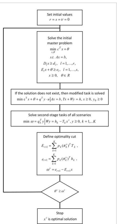
k= K until all the objective function values are zero. The algorithm scheme is shown in Fig. 1.

The algorithm is based on the decomposition method described by Bierge et al. [1]. However, several chang-es have been made.

Before the first iteration, the initial values are defined. Next, the main linear task (master) is solved. If the final solution of this problem does not exist, then, a modified task is solved. Next, the second-stage tasks (subproblem) are solved for all scenarios and vari-ables for the optimal cut are defined. Afterwards, the stop condition is checked, and if it is not satisfied, it-erations are repeated. The itit-erations are repeated un-til the required accuracy is obtained.

4. Scenario Aggregation Method

The scenario aggregation method was proposed by Rockafeller and Wets [10]. Later, Wets described the main aggregation principles in the scenario analysis and stochastic optimization [19]. Further, this meth-od has been applied in solving various specific prob-lems. In Jönsson et al. [6], the aggregation technique is applied to the two-stage production task when it is necessary to distribute the given budget for the pur-chase of product components. In many stages of un-certainty, optimization problems have been analysed for scenarios [11].

Subsequently, the scenario aggregation method was analysed in Cambou et al. [3], and the main criteria for applying this method were formulated, based on

Figure 1

A modified L-shaped algorithm

examples. The essence of the scenario aggregation method is described below.

The idea is that, when dealing with various subprob-lems and their optimal solutions, one can discover similarities and trends, and ultimately get a well-in-sured solution to the underlying problem [19]. The general approach in practice is based on the scenario analysis [6, 19].

If we have a stochastic optimization task described in Figure 1

Set initial values

0

 

s 

r

Solve the initial master problem , . . min , b Ax t s x cT x    , , ,1 , l r d

x

Dl  l  

, , ,1 , l s e

x

El  l  

R x0, 

If the solution does not exist, then modified task is solved 0 , 0 , , c

min TxqTyuAxb TxWyh x y0

Solve second-stage tasks of all scenarios K k y x T h Wy y q v k k T

k , 0, 1,...

min    

Define optimality cut

, ) ( , ) ( 1 1 1 1 k T v k K k k r k T v k K k k r h p T p E  



      x E er r v 1 1      v v _   Stop v

x is optimal solution

(6)

a probability space

(

Ø, ,P

)

where Ø is a set of possi-ble realizations, and P is the associated probability distribution, the problem is:

(

)

{

}

( ) ( )

min , , ,

x E g xξ = ∫g xξ dP ξ (22)

where x D R∈ ⊂ n, D is a set of feasible solutions de-termined by constraints, and g is the criterion function. Since the model depends on the random vector ξ and its probabilistic distribution P, it cannot be used as an appropriate simulation tool when we have only limited information on the distribution of random pa-rameters. In such cases, the scenario analysis is used most commonly [19].

In case the uncertainty is modelled by a few scenarios , 1, ,

k

s k= K and for each scenario _sk,_{one finds the} solution of subproblem P_k:

( )

{

}

min , | n

k

x g x s x D∈ ⊂R . (23)

Suppose we know how to get the solution to each in-dividual scenario taken. The problem is how to deal with different s-dependent vectors in solving the problem of combining them and obtaining a common solution [11].

Assuming that the optimal solution exists for all sce-narios _{s k}k, 1, ,₌ _K _{the optimal solution is:}

( )

{

}

min , |

k

k x

x ∈arg g x s x D∈ _. ₍₂₄₎

When the solution to each scenario is computed, they are analysed in order to find common trends or solu-tion clusters and determine how the solusolu-tion would be calculated, if the scenario s′ really appears. The average solution is calculated multiplying all solu-tions _xk_{by the probability of scenarios, and the}

aver-age solutions are analysed further. The ultimate goal of the analysis is to get one solution that can be used to make a decision.

Constructing an estimate indicating the average solution:

1

ˆ K k

k k

x p x

=

∑

, (25)

where _xk_{is the solution of the scenario}_{s k}k_{, 1, ,}₌ _K

and pk are probabilities (weights) of the scenario.

These probabilities are necessarily nonnegative, and up to 1 [19]. The solution xˆ does not depend on the scenario, i.e., in general, it will respond more to all the most likely events possible than specific solutions of the individual scenario solution xk. However, xˆ is not necessarily possible. The solution x is accept-able, if it is possible for each particular scenario, i.e.,

k

x D∈ for all s kk, 1, .= K

A stochastic optimization problem is defined below in which each scenario _sk_{relates to the probability of}

the scenario p_k:

( )

(

)

1

min K k , k ,

x k

∑

= p g x s

(26)

where x∈_skDk.

The optimal solution of the problem is _x*_.

5. Stochastic Simulation

Simulation is mainly used in the following cases: where it is impossible or very expensive to get data from a certain real process; where the system investi-gated is very complicated and cannot be described by mathematical equations having analytical solutions; where the system is described in a mathematical model, but it is impossible to get a solution by using analytical techniques; where it is impossible or very expensive to perform experiments of the mathemat-ical system model.

Simulation optimization coupling [2], illustrated in Fig. 2, is an active area in the field of stochastic pro-gramming. In this connection, the simulation is gen-erally used to generate scenarios in accordance with the probability distributions data [2].

Statistical modelling uses a selection of stochastic random variables, and is defined as experimentation with the model in time. Random values were sim-ulated by generating Gaussian values. The Normal or Gaussian law describes the distribution of such a random size obtained, by summing up a large number of other independent random variables that are not dominant among them.

(7)

Figure 2

Simulation optimization coupling [2]

The normal law is very often applied in practice. It is an idealized mathematical model for analysing data that are roughly normal. Therefore, in this work, random scenarios were generated according to the Gaussian law.

6. Optimization Using IBM ILOG

CPLEX

For solving optimization problems we used the IBM ILOG CPLEX Optimization Studio that was integrat-ed with Microsoft Visual Studio.

The IBM ILOG CPLEX Optimization Studio is an op-timization software package [5]. It enables a rapid de-velopment and deployment of decision optimization models using mathematical and constraint program-ming [5]. The efficiency of solution of a task depends on the CPLEX integration. Therefore, it is very im-portant to properly select and match all the parame-ters of the task.

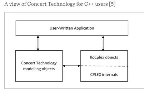
IBM ILOG CPLEX offers C, C++, Java, .NET, and Py-thon libraries that solve linear programming and re-lated problems [5]. Specifically, it solves linearly or quadratically constrained optimization problems, where the objective to be optimized can be expressed as a linear function or a convex quadratic function [5]. The variables in the model may be declared as contin-uous or further constrained to take only integer [5]. The program using the CPLEX Concert Technology to solve optimization problems is shown in Fig. 3. The optimization part of the user’s application pro-gram is captured in a set of interacting C++ modelling and solving objects that the application creates and controls [5]. Modelling objects are used to define the optimization problem. Solving objects in the instance

of IloCplex are used to solve models created by the modelling objects.

An IloCplex object reads a model, extracts its data, solves the problem, and answers queries on solution. The Concert Technology model consists of a set of C++ objects. Each variable, each constraint, each spe-cial ordered set (SOS), and the objective function in the model are all represented by objects of the appro-priate Concert Technology class.

The environment is the first object created in an appli-cation. The environment object needs to be available to the constructor of all other Concert Technology classes. After creating the environment, a Concert ap-plication is ready to create one or more optimization models. After an IloModel object has been construct-ed, it can be populated with modelling variables, con-straints, and objective function. The class IloCplex

solves a model. Query methods access information about the solution. CPLEX supports reading models from files and writing models to files in several lan-guages (e.g., LP format, MPS format).

We describe above the CPLEX model creation and the solving process used in our research.

First, we define the vector of solution variables as Ilo-NumVarArray.

Next, we define the first-stage and the second-stage objective function vectors as IloExpr, and add them to the model using model.add() method.

Now, we define the matrixes describing the left-hand of the first- and the second-stage constraints as

IloExprArray.

Next we define the first- and the second-stage con-straints as IloRangeArray, and add them to the model Figure 3

A view of Concert Technology for C++ users [5] Figure 2

Figure 3

User-Written Application

Concert Technology modelling objects

IloCplex objects

CPLEX internals

Figure 2

Figure 3

User-Written Application

Concert Technology modelling objects

IloCplex objects

(8)

using model.add() method.

Finally, we define created model as IloCplex model and solve it using the CPLEX solver method solve(). Next, we can apply the information of the solution to our further calculations. The main information of the solution are as follows:

_ cplex.getStatus() gets the status of the solution; _ cplex.getObjValue()gets the value of the objective

function;

_ cplex.getValues(vals, vars) gets the values of the

solution.

7. Investigation of the Proposed

Method

The scenario aggregation method was applied for solving a two-stage SLP task. The calculations were performed by a computer, which parameters are: In-tel(R) Core(TM) i7-4500U CPU @ 1,80 GHz 2.4 GHz, 8.00GB, x64-based processor. The program was im-plemented in the Microsoft Visual Studio 2012 C++ language, using the IBM ILOG CPLEX optimization package. The first two-stage task has 20 variables and 10 constraints in the first-stage, and 30 variables and 20 constraints in the second (20x30 task). The second two-stage task has 60 variables and 30 constraints in the first-stage, and 90 variables and 60 constraints in the second (60x90 task).

In the first case, the 2000 normally distributed scenar-ios were divided into 1, 2, 5, 10, 20, 50, 100, 200, 500, 1000 and 2000 groups. The calculations (2000 scenar-ios) were repeated 100 times for each case of division. The averaged results for all cases of division are pre-sented in Table 1 (average result = result of 2000 sce-narios repeated 100 times divided by 100).

The average value of the main (master) task objective function is TF=182.12.

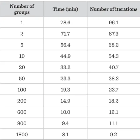
In the second case the 1800 normally distributed sce-narios were divided into 1, 2, 5, 10, 20, 50, 100, 200, 600, 900 and 1800 groups. The calculations (1800 scenari-os) were repeated 100 times for each case of division. The averaged results for all cases of division are pre-sented in Table 2 (average result = result of 1800 sce-narios repeated 100 times divided by 100).

The average value of the main (master) task objective function is TF =299.07.

The results indicate that by increasing the number of groups, the computation time and the number of iterations required to achieve the optimal value, de-Table 1

Averaged results of calculation (20x30 task)

Number of

groups Time (min) Number of iterations

1 22.2 34.3

2 20.0 30.2

5 17.1 26.3

10 15.3 23.1

20 13.0 20.2

50 11.0 17.1

100 9.3 14.2

200 7.8 12.1

500 5.7 8.7

1000 4.7 7.1

2000 4.1 6.1

Table 2

Averaged results of calculation (60x90 task)

Number of

groups Time (min) Number of iterations

1 78.6 96.1

2 71.7 87.3

5 56.4 68.2

10 44.9 54.3

20 33.2 40.7

50 23.3 28.3

100 19.3 23.7

200 14.9 18.2

600 10.0 12.1

900 9.4 11.1

(9)

crease. Dependence of time on the number of groups is shown in Fig. 4.

Figure 4

Dependence of time (y axis) on the number of groups (x axis)

Figure 5

Dependence of the number of iterations (y axis) on the number of groups (x axis)

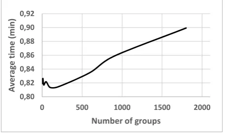
Figure 6

Dependence of the average time of one iteration calculation (y axis) on the number of groups (x axis) (20x30 task)

Figure 7

Dependence of the average time of one iteration calculation (y axis) on the number of groups (x axis) (60x90 task)

0,0 20,0 40,0 60,0 80,0 100,0

1 10 100 1000 10000

Ti

me (mi

n)

Number of groups

60x90 task 20x30 task

1,0 10,0 100,0

1 10 100 1000 10000

Number

of

ite

ra

tio

ns

Number of groups 60x90 task 20x30 task

0,64 0,65 0,66 0,67 0,68 0,69 0,70

0 500 1000 1500 2000

Aver

ag

e

tim

e (m

in

)

Number of groups

0,80 0,82 0,84 0,86 0,88 0,90 0,92

0 500 1000 1500 2000

Av

erag

e

time (

mi

n)

Number of groups Dependence of the number of iterations on the

num-ber of groups is shown in Fig. 5.

Dependence of the average time of one iteration cal-culation on the number of groups is shown in Fig. 6 (20x30 task) and Fig. 7 (60x90 task).

As we can see, the optimal time of one iteration cal-culation was obtained when the number of groups is between 100 and 200, i.e. one group have contain about 10–20 scenarios. When the number of groups increase, the calculation time of the one iteration in-creases too, because the number of constraints of the main (master) task increases respectively.

When we use our proposed two-stage SLP problem decomposition algorithm modification, we must en-sure the solution existence for every scenario. For

that purpose, the values of parameter u related to solution existence were investigated.

At the beginning, the parameter value u was set to

u = 1. Then it was reduced to 0.0001, and the problem was solved. The process was carried out as long as the solution existed.

The calculation results showed, that the minimal u

value which can ensure solution existence solving such tasks, is u=0.001.

8. Conclusion

(10)

The decomposition method, based on Sample Aver-age Approximation for solving SLP problems, is pre-sented, where the stochastic variables are described by an absolutely continuous probability law.

The investigation result obtained on choice of parame-ter u of our proposed two-stage SLP problem decompo-sition method modification algorithm shows that mini-mal value, which ensure solution existence, is u=0.001. The efficient CPLEX integration has been proposed for solving SLP problems by the L-shaped algorithm which enables us to adapt integration parameters to specific problems.

The obtained results show that the number of itera-tions decreases by increasing the number of scenario groups (see Fig. 5), concurrently the overall calcula-tion time decreases for the same accuracy (see Fig. 4).

The aggregation of the scenarios into 100-200 groups gives the best average execution time per iteration solving the SLP by modified Lshaped algorithm, if the following conditions are met: the number of variables reaches up to 100; random scenarios are generated according to the Gaussian law; number of the scenarios is about 2000. Increasing the number of groups, the average calculation time of one itera-tion increases as well (see Figs. 6 and 7). This is due to the fact that if the number of groups increases, the number of constraints of the main (master) task in-creases, respectively.

The disadvantage of the method is that the different classes of problems can correspond to different num-bers of optimal groups. If we do not know the number of optimal groups, our choice may be irrational.

References

1. Birge, J. R., Louveauxl, F. V. Introduction to Stochastic

Programming. Springer, New York, 2011. hhttps://doi.

org/10.1007/978-1-4614-0237-4

2. Borodin, V., Bourtembourg, J., Hnaien, F., Labadie, N. COTS Software Integration for Simulation Optimi-zation Coupling: Case of ARENA and CPLEX Prod-ucts. Working Paper EMSE CMP–SFL, 2018. https:// hal-emse.ccsd.cnrs.fr/emse-01687555/document. Ac-cessed on January 27, 2018.

3. Cambou, M., Filipović, D. Model Uncertainty and Sce-nario Aggregation. Mathematical Finance, Forthcom-ing, Swiss Finance Institute Research Paper No. 14-38.

February 2, 2014. https://doi.org/10.2139/ssrn.2441328

4. Fountoulakis, K., Gondzio, J. Performance of First- and Second-Order Methods for L1-Regularized Least Squares Problems. Computational Optimization

and Applications, 2016, 65(3), 605-635. https://doi.

org/10.1007/s10589-016-9853-x

5. IBM Inc. IBM ILOG CPLEX Optimization Studio Get-ting Started with CPLEX (Version 12 Release 6). IBM Corporation, 2014.

6. Jönsson, H., Jörnsten, K., Silver, E. A. Application of the Scenario Aggregation Approach to a Two-stage, Stochastic, Common Component, Inventory Problem with a Budget Constraint. European Journal of

Op-erational Research, 1993, 68(2), 196-211. https://doi.

org/10.1016/0377-2217(93)90303-5

7. King, A. J., Wallace, S. W. Modeling with Stochastic Pro-gramming. Springer Series in Operations Research and

Financial Engineering, Springer, New York, 2012. ISBN 978-0-387-87817-1.

8. Ogbe, E., Li, X. A New Cross Decomposition Method for Stochastic Mixed-Integer Linear Programming. Eu-ropean Journal of Operational Research, 2017, 256(2),

487-499. https://doi.org/10.1016/j.ejor.2016.08.005

9. Rahmaniani, R., Crainic, T. G., Gendreau, M., Rei, W. The Benders Decomposition Algorithm: A Litera-ture Review. European Journal of Operational

Re-search, 2017, 259(3), 801-817. https://doi.org/10.1016/j.

ejor.2016.12.005

10. Rockafellar, R. T., Wets, R. J.-B. Scenarios and Policy Aggregation in Optimization Under Uncertainty. IIASA Working Paper. IIASA, Laxenburg, Austria: WP-87-119, 1987. http://pure.iiasa.ac.at/id/eprint/2933/1/WP-87-119.pdf. Accessed on June 25, 2017.

11. Rockafellar, R. T., Wets, R. J.-B. Scenarios and Policy Aggregation in Optimization under Uncertainty. Math-ematics of Operations Research, 1991, 16(1), 119-147.

https://doi.org/10.1287/moor.16.1.119

12. Sakalauskas, L. Application of the Monte-Carlo Meth-od to Nonlinear Stochastic Optimization with Linear Constraints. Informatica, 2004, 15(2), 271-282. ISSN 0868-4952.

13. Schulzea, T., Grothey, A., McKinnon, K. A Stabilised Scenario Decomposition Algorithm Applied to Sto-chastic Unit Commitment Problems. European Journal

of Operational Research, 2017, 261(1), 247-259. https://

(11)

14. Shabbir, A., Shapiro, A. The Sample Average Approxi-mation Method for Stochastic Programs with Integer Recourse. ISyE Technical Report, 2002. https://www2. isye.gatech.edu/~sahmed/saasip.pdf. Accessed on June 21, 2017.

15. Sun, L., Liu, W., Chai, T., Wang, H., Zheng, B. Crane Scheduling of Steel-Making and Continuous Casting Process Using the Mixed-Timed Petri Net Modelling via CPLEX Optimization. IFAC Proceedings Volumes, 2011,

44(1), 9482-9487.

https://doi.org/10.3182/20110828-6-IT-1002.00170

16. Ušpurienė, A., Sakalauskas, L., Giuliani, S., Meloni, C. ABC Model for Economic Development of a Firm. Technological and Economic Development of

Econo-my, 2016, 22(4), 512-531. https://doi.org/10.3846/2029

4913.2016.1190420

17. Vamanan, M., Wang, Q., Batta, R., Szczerba, R. J. Inte-gration of COTS Software Products ARENA & CPLEX for an Inventory/Logistics Problem. Computers &

Op-erations Research, 2004, 31(4), 533-547. https://doi.

org/10.1016/S0305-0548(03)00010-8

18. Wang, T., Wang, S., Meng, Q. Liner Ship Fleet Planning: Models and Algorithms, Part Two: Mathematical Mod-eling, Elsevier, 2017, 61-72. ISBN: 978-0-12-811502-2. 19. Wets, R. J.-B. The Aggregation Principle in

Scenar-io Analysis and Stochastic OptimizatScenar-ion. Algorithms and Modelling in Mathematical Programming,

Spring-er-Verlag, Berlin, Heidelberg, 1989, 91-113. https://doi.

org/10.1007/978-3-642-83724-1_4