Predictive Functional Control for Fractional Order System

(1)

Predictive Functional Control for Fractional Order

System

Morteza Abdolhosseini, Nooshin Bigdeli

Abstract – The fractional calculus is the area of

mathematics that handles derivatives and integrals of any arbitrary order (fractional or integer, real or complex order). Predictive Functional Control (PFC) is one of the most popular methods of model predictive control. The implementation of the predictive functional controller (PFC) on the fractional order systems has been presented in this paper. The effect of various approximations, sensitivity analysis, tuning of predictive functional controller parameters, the effect of delay and noise analysis of the fractional-order system has been considered. It has been shown that, in fractional order system,predictive functional control gives acceptable results.

Keywords – Fractional Order Systems, Predictive

Functional Control, Model-Based Predictive Control, Closed-Loop Control Performance.

I. I

NTRODUCTION

Model predictive control (MPC) or predictive functional control(PFC) strategies have experienced intensive study in control theory and engineering since the 1970s. Typically, there are three main MPC design methods: finite impulse response (FIR) or step response models, transfer function models and state space models. MPC based on state space models can be seen in predictive functional control [1]. PFC has been pioneered by Richalet tocontrol dynamically fast systems. It uses concepts of prediction and control horizons as other MPC variants. The difference is that in PFC, instead of minimizing a cost function, the control command is derived by making a few future output points equal to their corresponding points in the desired trajectory. With this idea, in PFC, instead of implementing an optimization problem, just a few algebraic equations are solved and this is why the computational complexity is reduced considerably [2]. This control method has been widely used in robot, chemical engineering process, radar and missile [3].

The fractional calculus is the area of mathematics that handles derivatives and integrals of any arbitrary order (fractional or integer, real or complex order).Although the concept of the fractional calculus was discussed in the same time interval of integer order calculus, the complexity and the lack of applications postponed its progress till a few decades ago. During the last few decades, most of the dynamical systems based on the integer-order calculus have been modified into the fractional order domain due to the extra degrees of freedom and the flexibility which can be used to precisely fit the experimental data much better than the integer-order modeling and fractional calculus has become a powerful tool in describing the dynamics of complex systems which appear frequently in several branches of science and engineering. Therefore fractional differential

equations and their numerical techniques find numerous applications in the field of viscoelasticity, robotics, feedback amplifiers, electrical circuits, control theory, electro analytical chemistry, fractional multi-poles, chemistry and biological sciences [4].

In recent years, the application of fractional order system control has become a new topic. In [5] the standard H∞ control problem for continuous-time fractional linear time-invariant single-input–single-output systems has been stated. In [6] several decomposed hybrid structures of the fractional order fuzzy PID controller has been proposed. In [7] classical proper PID controllers have been designed for linear time invariant fractional-order systems with time delays. In [8] has been presented a LMI-based design method of robust control for fractional-order uncertain systems with the fractional order 0 < α <2. The sufficient condition for the robust asymptotical stability of the fractional-order closed loop control systems was first presented. In [9] Fractional order sliding mode controller has been suggested for antilock braking systems to regulate the slip to the desired value.

Predictive functional control has been in use in the process industries during the last 30 years, where it has become an industry standard due to intrinsic ability to handle input and state constrain for large scale multivariable plants. In [10] design and implementation of a speed controller based on predictive functional control for the PMSM system has been investigated. In [11] has been used the problem of conveyor belt speed control in a factory for producing stone wool by predictive functional control. In [12] predictive functional control technique has been applied for temperature control of a bench-scale batch reactor and implemented in Programmable Logic Controller (PLC). In [13]has been presented a partially decoupled design of the state space predictive functional control for MIMOprocesses. The multivariable process has been first treated into MISO process by a simple Cramer’s rule solution to linear equations which has been provided a balance between model complexity and control system design, and then the has been derived MISO process based extended state space predictive functional control has been used.

(2)

Predictive Functional Control (FPFC). PFC is a predictive method based on the predictive control theory. This control method has the following properties: simple calculation, strong robustness, disturbance attenuation and high control precision. In this paper, the implementation of the predictive functional controller (PFC) on the fractional order systems is presented in this paper. The effect of various approximations, sensitivity analysis, tuning of predictive functional controller parameters, the effect of delay and noise analysis of the fractional-order system is considered.

The rest of this paper is organized as follows. In next Section, fundamental of fractional order is described. The PFC method is presented in Section 3. PFC’s application to the fractional order system is discussed in Section 4. Finally, conclusions are brought in Sections 5.

II. F

UNDAMENTAL OF

F

RACTIONAL

O

RDER

The fractional calculus theory is in fact the random ordercalculus theory, which is the extension of traditional calculus.

a𝐷𝑡𝛼 =

𝑑𝛼

𝑑𝑡𝛼, 𝑅𝑒(𝛼) > 0

1 , 𝑅𝑒(𝛼) = 0 (𝑑𝜏)𝑡 𝛼

𝑎 , 𝑅𝑒(𝛼) < 0

(1)

In this formula, a and t are the limits of the operation and α represents order of fractional calculus.Three kindsof definitions of fractional calculus used commonly are the following.

I. Grunwald-Letnikov’s definition

a𝐷𝑡𝛼𝑓 𝑡 = lim𝑕 →0𝑕−𝛼 −1 𝑗 𝑡−𝛼

𝑕 𝑗 =0

𝛼

𝑗 𝑓(𝑡 − 𝑗𝑕)

(2)

In this formula, 𝑡−𝛼

𝑕 expresses integral part of the

number 𝑡−𝛼

𝑕 , 𝛼

𝑗 is binomial coefficient and 𝑓 𝑡 is

continual function in the sector [α, t].

II. Riemann-Liouville’s definition

a𝐷𝑡𝛼𝑓 𝑡 = 𝑑𝑛

𝑑𝑡𝑛 1

𝛤(𝑛−𝛼)

𝑓(𝜏)

(𝑡−𝜏)𝑛 −𝛼 −1𝑑𝜏 𝑡

𝑎

0≤n-1<α<n

(3)

In this formula, Γ (.) is Gamma function.

III. Caputo’s definition

a𝐷𝑡𝛼𝑓 𝑡 = 1

𝛤 𝑛−𝛼 𝑡 − 𝜏 𝑛−𝛼 −1 𝑡

𝑎 𝑓

𝑛 _{(𝜏)𝑑𝜏}

0≤n-1<α<n ,n∈N[17]

(4)

III. PFC

M

ETHOD

Predictive functional control has laws similar to the classical predictive control, such that each method is used one model to predict the future output of the system. In predictive functional control, the control law to form a linear combination of a set of basic functions is considered and the basic functions weight on the linear combination should be calculated. Choice of basic functions is takes placed based on the process characteristics and the reference input. The structure of the control law can be defined as follows:

𝑢(𝑘 + 𝑖) = 𝜇𝑛

𝑁

𝑛=1

𝑢𝑏𝑛(𝑖) (5)

whereμ_n are the basis functions coefficients in the linear combination and N are the number of basic functions. ubn i are values of the basis function at time

k + i.The choice of basis functions depend on the nature of the process and the input reference and generally, canonical functions are used, e.g., step, ramp.

(6)

𝑢(𝑘 + 𝑖) = 𝜇1 𝑘 + 𝜇2 𝑘 × 𝑖

PFC algorithm, a set of future control variables find that process out as far as possible have been closed to the reference trajectory. The reference trajectory can be computed by an exponential equation(7):

𝑦𝑟 𝑘 + 𝑖 = 𝑤 𝑘 + 𝑖 − 𝜆𝑖[𝑤 𝑘 − 𝑦 𝑘 ] (7)

where, i=1,2,…,Hi are the total number of the coincidence points. yr k + i are the values of the reference trajectory

at time k + i. w k are the set point values and y k are the

actual process outputs. λi= e−TsTrare the parameter that specifies the desired tracking speed , Ts is sample time and

Tr is the desired time response of the closed loop system.

State equation of system is as follows:

𝐿 𝑘 + 1 = 𝐴𝐿 𝑘 + 𝐵𝑢 𝑘 𝑦 𝑘 = 𝐶𝑙(𝑘)

(8)

According to (8) and (6), the predicted future process output is given by the following equation:

𝑦𝑚 𝑘 + 𝑖 = 𝐶𝐴𝑖𝐿 𝑘

+𝐶 𝐴𝑖−1_{+ 𝐴}𝑖−2_{+ ⋯ + 𝐼 𝐵𝜇} 1 𝑘

+𝐶 𝐴𝑖−2_{+ 2𝐴}𝑖−3_{+ ⋯ + (𝑖 − 1)𝐼 𝐵𝜇} 2 𝑘

(9)

where, ym k + i are the output of the prediction model at

time k + i. Considering the model mismatch, the impact of various kinds of interference and noise, there are some errors between forecasted model output and process. The prediction error is given by:

𝑒 𝑘 + 𝑖 = 𝑦 𝑘 − 𝑦𝑚(𝑘) (10)

The following cost function guarantees an optimal transition of the system output as closely as possible to the reference trajectory:

𝑗 = [𝑦𝑚 𝑘 + 𝑖 + 𝑒 𝑘 + 𝑖 − 𝑦𝑟(𝑘 + 𝑖)]2 𝐻2

𝑖=𝐻1

(11)

In the relation control efforts only two factors of the basic functions, namely μ₁(k)and μ₂ k are unknown. In order to get unknown parameters easily, rewrite (11) to (12):

𝑗 = [𝑦𝑚 𝑘 + 𝐻1 + 𝑒 𝑘 + 𝐻1 − 𝑦𝑟 𝑘 + 𝐻1 ]2

+[𝑦𝑚 𝑘 + 𝐻2 + 𝑒 𝑘 + 𝐻2 − 𝑦𝑟 𝑘 + 𝐻2 ]2

(12)

Substituting (7), (9) in to (12) gives (13):

𝑗 = [𝑋1 𝑘 + 𝑀11𝜇1 𝑘 + 𝑀12𝜇2(𝑘)]2

+[𝑋2 𝑘 + 𝑀21𝜇1 𝑘 + 𝑀22𝜇2(𝑘)]2

(13)

where

𝑋1 𝑘 = 𝐶𝐴𝐻1𝐿 𝑘 + 𝑒 𝑘 + 𝐻1 − 𝑦𝑟(𝑘 + 𝐻1)

𝑋2 𝑘 = 𝐶𝐴𝐻2𝐿 𝑘 + 𝑒 𝑘 + 𝐻2 − 𝑦𝑟(𝑘 + 𝐻2)

𝑀11= 𝐶 𝐴𝐻1−1+ 𝐴𝐻1−2+ ⋯ + 𝐼 𝐵

𝑀12= 𝐶 𝐴𝐻1−2+ 2𝐴𝐻1−3+ ⋯ + (𝐻1− 1)𝐼 𝐵

𝑀21= 𝐶 𝐴𝐻2−1+ 𝐴𝐻2−2+ ⋯ + 𝐼 𝐵

𝑀22= 𝐶 𝐴𝐻2−2+ 2𝐴𝐻2−3+ ⋯ + (𝐻2− 1)𝐼 𝐵

(3)

unknown parameters μ₁(k)and μ₂(k), the following equation has been obtained:

𝑢(𝑘) = 𝜇1 𝑘 = 𝑆𝑦𝑦 𝑘 + 𝑆𝑙𝐿 𝑘 + 𝑆𝑤𝑤(𝑘) (15)

where

𝑆𝑦 = 𝑄 𝑄3𝑀12− 𝑄2𝑀11 1 − 𝜆𝐻1

+𝑄 𝑄3𝑀22− 𝑄2𝑀21 1 − 𝜆𝐻2

𝑆𝑙 = 𝑄 𝑄3𝑀12− 𝑄2𝑀11 𝐶 𝐴𝐻1− 𝐼

+𝑄 𝑄3𝑀22− 𝑄2𝑀21 𝐶 𝐴𝐻2− 𝐼

𝑆𝑤 = −𝑆𝑦

𝑄1= 𝑀112 + 𝑀212

𝑄2= 𝑀122 + 𝑀222

𝑄3= 𝑀11𝑀12+ 𝑀21𝑀22

𝑄 = 1

(𝑄1𝑄2− 𝑄32)

(16)

According to (15), the parameter μ₁ k will be existed only if Q has been existed. This will be guaranteed when the parameters of controller H1 and H2 have been selected

properly.

However, using equation (16) and (8), relationship of the closed-loop system state-space can be written as

:

𝐿 𝑘 + 1 = 𝐴𝑐𝐿 𝑘 + 𝐵𝑐𝑢(𝑘) (17)

where Ac= A + BSl+ BSlC. A, B and Care constants and

has been identified to be offline. Sl, Sy and Swwith the

right choice of parameters H1 and H2 has been limited.

The set point values w(k) have been bounded for all the time. According to Lyapunov stability theory, the system is stable when all the eigenvalues of Ac are less than

one[18]. The stability condition can be defined as:

𝜆𝑖(𝐴𝑐) < 1 (18)

IV. FOS-PFC

(F

RACTIONAL

O

RDER

S

YSTEM

-P

REDICTIVE

F

UNCTIONAL

C

ONTROL

)

In part of article, the design of predictive functional control for fractional-order system will be done. For this purpose, the fractional-order system has been approximated with a good approximation to an integer order system and then for this integer order system, a predictive functional control has been designed properly and variant analysis on this controller will be done.

In this paper will be focused on Podlubny commensurate fractional-order system [19] has been presented as follows:

𝐺 𝑠 = 1

0.8𝑠2.2_{+ 0.5𝑠}0.9_{+ 1} (19)

Podlubny system step response has been plotted in Fig 1:

Fig.1. System step response.

The effects of variant approximation on this system will be investigated in this paper. The fractional-order system has been converted to the integer order system by a good approximation. Approximation methods are as follows:

First Method:

The method is based on the approximation of a function of the form:

𝐻 𝑠 = 𝑠𝜇_{, 𝜇𝜖𝑅}+ ₍₂₀₎

by a rational function:

𝐻 𝑠 = 𝐶 1 + 𝑠 𝑤𝑘

1 + 𝑠 𝑤′𝑘 𝑁

𝑘=−𝑁

(21)

using the following set of synthesis formulas:

𝑤′0= 𝛼−0.5𝑤𝑢 ; 𝑤0= 𝛼0.5𝑤𝑢

𝑤′𝑘+1

𝑤′

𝑘

=𝑤𝑘 +1 𝑤𝑘

= 𝛼𝜂 > 1

𝑤′𝑘+1

𝑤𝑘

= 𝜂 > 0 ; 𝑤𝑘 𝑤′𝑘

= 𝛼 > 0 ;

𝑁 =𝑙𝑜𝑔⁡(𝑤𝑁 𝑤0)

𝑙𝑜𝑔⁡(𝑎𝜂) ; 𝜇 =

𝑙𝑜𝑔⁡(𝑎) 𝑙𝑜𝑔⁡(𝑎𝜂)

(22)

with wu being the unit gain frequency and the central

frequency of a band of frequencies geometrically distributed around it. That is,wu = wbwh , wb, whare the

low and high transitional frequencies[20].

Fractional-order system with oustaloup approximation has been approximated to integer-order system and then prediction functional controller will be designed. Here,

H1= 135, H2= 165, Tr = 20sec, Ts = 0.1sec, wb=

0.001Hz, wh = 1000HzandN = 1 have been considered

that the best result has been achieved. Result of predictive functional control design with this approximation has been shown in Fig 2:

Fig.2. Design of predictive functional control by oustaloup approximation.

0 5 10 15 20 25 30

0 0.5 1 1.5

Time [sec]

A

m

p

li

t

u

d

(4)

the predictive controller is an ideal but order of the system with oustaloup approximation has been eight (assuming the above parameters) and this method has been leaded to major changes in the step response. Thus the overall result is not good and analysis on this method will not be made.

Second Method:

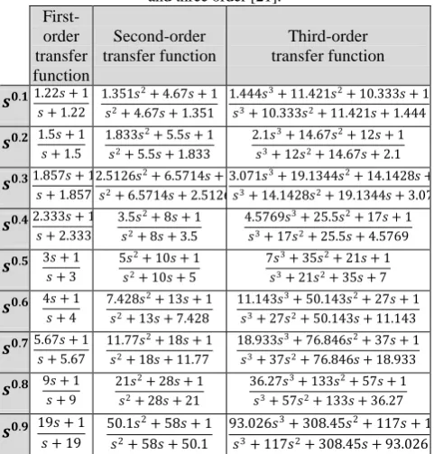
In the paper [21], a good approximation has been suggested in the table where𝑠𝜇_and_{𝜇 =}₀_.₁_,₀_.₂_{, … ,}₀_._{9 in}

terms of transfer functions into one, two, three and four order have been expressed. Here, Podlubnysystem has been convertedintothe belowform:

𝐺 𝑠 = 1

0.8𝑠2.2_{+ 0.5𝑠}0.9_{+ 1}

= 1

0.8𝑠2_𝑠0.2_{+ 0.5𝑠}0.9_{+ 1}

(23)

According to Table1 and 2, instead of

𝑠

0.9and

𝑠

0.2

,

transfer functionsone, two, three and four order have beenplacementandresultshave been observed.

Table 1: approximation of 𝑠𝜇_{into transferfunctionsof one, two,}

and three order [21].

First-order transfer function

Second-order transfer function

Third-order transfer function

𝒔𝟎.𝟏1.22𝑠 + 1 𝑠 + 1.22

1.351𝑠2_{+ 4.67𝑠 + 1} 𝑠2_{+ 4.67𝑠 + 1.351}

1.444𝑠3_{+ 11.421𝑠}2_{+ 10.333𝑠 + 1} 𝑠3_{+ 10.333𝑠}2_{+ 11.421𝑠 + 1.444}

𝒔𝟎.𝟐 1.5𝑠 + 1 𝑠 + 1.5

1.833𝑠2_{+ 5.5𝑠 + 1} 𝑠2_{+ 5.5𝑠 + 1.833}

2.1𝑠3_{+ 14.67𝑠}2_{+ 12𝑠 + 1} 𝑠3_{+ 12𝑠}2_{+ 14.67𝑠 + 2.1}

𝒔𝟎.𝟑1.857𝑠 + 1_{𝑠 + 1.857}2.5126𝑠2+ 6.5714𝑠 + 1

𝑠2_{+ 6.5714𝑠 + 2.5126}

3.071𝑠3_{+ 19.1344𝑠}2_{+ 14.1428𝑠 + 1} 𝑠3_{+ 14.1428𝑠}2_{+ 19.1344𝑠 + 3.071}

𝒔𝟎.𝟒2.333𝑠 + 1 𝑠 + 2.333

3.5𝑠2_{+ 8𝑠 + 1} 𝑠2_{+ 8𝑠 + 3.5}

4.5769𝑠3_{+ 25.5𝑠}2_{+ 17𝑠 + 1} 𝑠3_{+ 17𝑠}2_{+ 25.5𝑠 + 4.5769}

𝒔𝟎.𝟓 3𝑠 + 1 𝑠 + 3

5𝑠2_{+ 10𝑠 + 1} 𝑠2_{+ 10𝑠 + 5}

7𝑠3_{+ 35𝑠}2_{+ 21𝑠 + 1} 𝑠3_{+ 21𝑠}2_{+ 35𝑠 + 7}

𝒔𝟎.𝟔 4𝑠 + 1 𝑠 + 4

7.428𝑠2_{+ 13𝑠 + 1} 𝑠2_{+ 13𝑠 + 7.428}

11.143𝑠3_{+ 50.143𝑠}2_{+ 27𝑠 + 1} 𝑠3_{+ 27𝑠}2_{+ 50.143𝑠 + 11.143}

𝒔𝟎.𝟕5.67𝑠 + 1_{𝑠 + 5.67} 11.77𝑠2+ 18𝑠 + 1

𝑠2_{+ 18𝑠 + 11.77}

18.933𝑠3_{+ 76.846𝑠}2_{+ 37𝑠 + 1} 𝑠3_{+ 37𝑠}2_{+ 76.846𝑠 + 18.933}

𝒔𝟎.𝟖 9𝑠 + 1 𝑠 + 9

21𝑠2_{+ 28𝑠 + 1} 𝑠2_{+ 28𝑠 + 21}

36.27𝑠3_{+ 133𝑠}2_{+ 57𝑠 + 1} 𝑠3_{+ 57𝑠}2_{+ 133𝑠 + 36.27}

𝒔𝟎.𝟗 19𝑠 + 1

𝑠 + 19

50.1𝑠2_{+ 58𝑠 + 1}

𝑠2_{+ 58𝑠 + 50.1}

93.026𝑠3_{+ 308.45𝑠}2_{+ 117𝑠 + 1}

𝑠3_{+ 117𝑠}2_{+ 308.45𝑠 + 93.026}

Table 1: approximation of 𝑠𝜇_{into transferfunctionsof four order}

[21].

Fourth-order

transfer function

𝒔𝟎.𝟏 1.518𝑠4+ 21.529𝑠3+ 44.596𝑠2+ 18.222𝑠 + 1

𝑠4_{+ 18.222𝑠}3_{+ 44.596𝑠}2_{+ 21.529𝑠 + 1.518}

𝒔𝟎.𝟐 2.316𝑠4+ 29.333𝑠3+ 56𝑠2+ 21𝑠 + 1

𝑠4_{+ 21𝑠}3_{+ 56𝑠}2_{+ 29.333𝑠 + 2.316}

𝒔𝟎.𝟑 3.57𝑠4+ 40.63𝑠3+ 71.546𝑠2+ 24.57𝑠 + 1

𝑠4_{+ 24.57𝑠}3_{+ 71.546𝑠}2_{+ 40.63𝑠 + 3.57}

𝒔𝟎.𝟒 5.594𝑠4+ 57.538𝑠3+ 93.5𝑠2+ 29.333𝑠 + 1

𝑠4_{+ 29.333𝑠}3_{+ 93.5𝑠}2_{+ 57.538𝑠 + 5.594}

𝒔𝟎.𝟓 9𝑠4+ 84𝑠3+ 126𝑠2+ 36𝑠 + 1

𝑠4_{+ 36𝑠}3_{+ 126𝑠}2_{+ 84𝑠 + 9}

𝒔𝟎.𝟔 15.076𝑠4+ 128.143𝑠3+ 177.428𝑠2+ 46𝑠 + 1

𝑠4_{+ 46𝑠}3_{+ 177.428𝑠}2_{+ 128.143𝑠 + 15.076}

𝒔𝟎.𝟕 26.965𝑠4+ 209.38𝑠3+ 267.54𝑠2+ 62.67𝑠 + 1

𝑠4_{+ 62.67𝑠}3_{+ 267.54𝑠}2_{+ 209.38𝑠 + 26.965}

𝒔𝟎.𝟖 54.41𝑠4+ 386.91𝑠3+ 456𝑠2+ 96𝑠 + 1

𝑠4_{+ 96𝑠}3_{+ 456𝑠}2_{+ 386.91𝑠 + 54.41}

𝒔𝟎.𝟗 147.04𝑠4+ 959.64𝑠3+ 1042.36𝑠2+ 196𝑠 + 1

𝑠4_{+ 196𝑠}3_{+ 1042.36𝑠}2_{+ 959.64𝑠 + 147.04}

With the approximation of 𝑠0.2_and

_𝑠

0.9 _{with first-order} transfer function, transfer function

𝐺

₁has been obtained as follows:

𝐺1=

1

0.8𝑠2 1.5𝑠+1

𝑠+1.5 + 0.5 19𝑠+1

𝑠+19 + 1

=

𝑠2_{+ 20.5𝑠 + 28.5}

1.2𝑠4_{+ 23.6𝑠}3_{+ 25.7𝑠}2_{+ 35.25𝑠 + 29.25}

24)

)

In the Fig 3predictive functionalcontrollerstep responseforthetransfer function

𝐺

₁has beenshown.

Fig.3. Predictive functional controller step response for the transfer function 𝐺1.

With the approximation of

𝑠

0.2 and

𝑠

0.9 with second-order transfer function, transfer function

G

₂has been obtained as follows:

𝐺2=

63.5𝑠3_{+ 370.933𝑠}2_+→

1.4664𝑠6_{+ 89.4512𝑠}5_{+ 355.5166𝑠}4_+→

381.864𝑠 + 91.8333

497.1150𝑠3_{+ 616.9297𝑠}2_{+ 437.771𝑠 + 92.7498}

25) )

In the Fig4 predictive functional controller step response for the transfer function G2 has been shown.

(5)

𝑠

0.2 and

𝑠

0.9with

third-order transfer function, transfer function 𝐺3 has been

obtained as follows:

𝐺3=

129𝑠5_{+ 1727.1𝑠}4_{+ 5512.9𝑠}3_+→

1.68𝑠8_{+ 208.296𝑠}7_{+ 1948.4𝑠}6_{+ 5741.6𝑠}5_+→

5887𝑠2_{+ 2012.4𝑠 + 195.3546}

8465.1𝑠4_{+ 9715.4𝑠}3_{+ 7149.5𝑠}2_{+ 2142.6𝑠 + 196.4046}

(26)

In the Fig5 predictive functional controller step response for the transfer function 𝐺3 has been shown.

Fig.5. Predictive functional controller step response for the transfer function 𝐺3.

With the approximation of

𝑠

0.2 and

𝑠

0.9with fourth-order transfer function, transfer function 𝐺4has been

obtained as follows:

𝐺4 =

217𝑠7_{+ 5214.4𝑠}6_{+ 33855𝑠}5_+→

1.8534𝑠10_{+ 386.7406𝑠}9_{+ 6650.7𝑠}8_{+ 37277𝑠}7_+→

84423𝑠4_{+ 87857𝑠}3_{+ 38797𝑠}2_+→

92712𝑠6_{+ 138034𝑠}5_{+ 153460𝑠}4_+→

6535.7𝑠 + 340.5446

112990𝑠3_{+ 43025𝑠}2_{+ 6777𝑠 + 342}

(27)

In the Fig 6 predictive functional controller step response for the transfer function 𝐺4 has been shown.

Fig.6. Predictive functional controller step response for the

𝐺3.

From Figs3 –6 have been conclusioned that the approximation of order 3 and 4 does not give a good result. Fig 3 and Fig 4have a better response, but in this paper the first order approximation of system G has been used and sensitivity analysis, tuning of predictive functional controller parameters, the effect of delay and

input noise analysis of the fractional-order system have been checked.

1-Sensitivity analysis

To examine the sensitivity analysis, ageneral formas follows has been considered thattheinitial values are𝐴 = 0.8, 𝐵 = 0.5, 𝐶 = 1, 𝛼 = 2.2 and 𝛽 = 0.9and the effects ofchanging ofthese parameters have been surveyed. InTable2for± 5%and± 10% changes of initial values of the parameters 𝐴, 𝐵 and 𝐶and± 0.1and± 0.2changesthe initial value of the parameters 𝛼 and 𝛽 change has been investigated over shoot, rise time, settling time and stability. Using Table 2 has been observed that the fractional-order predictive controller is robust by changing of parameters Band C, but by changing of the parameters of A, α and β isn’t robust.

𝐺 = 1

𝐴𝑠𝑎_{+ 𝐵𝑠}𝛽 _{+ 𝐶} (28)

Table2: Sensitivity analysis.

Stability Settling

time(sec) Rise

time(sec) Overshoot

(%)

stable 9.9

2.2 28

2

α 2.1 36 2.1 15.5 stable

unstable -

-

-2.3

unstable -

- -

2.4

stable 8

2.5 9

0.7

β 0.8 19 2.1 15.7 stable

stable 43.6

1.85 48

1

unstable -

- -

1.1

stable 6.9

1.1 22

0.72

A

stable 16.2

2.1 25

0.76

stable 60

1.8 50

0.84

unstable -

- -

0.88

stable 43

1.7 35

0.45

B

stable 32.4

1.8 34

0.48

stable 22.1

2 31

0.53

stable 19.6

2 30

0.55

stable 64

1.9 54

0.9

C

stable 40

1.9 45

0.95

stable 18.6

2 23

1.05

stable 13.3

2.2 18

(6)

system for the changes of Table2. According to equation (18), the eigen values placed out side the unit radius circle, will be unstable.

Fig.7. Stability analysis by changing α.

From Fig7 has been observed that for 𝛼 = 2 and

𝛼 = 2.1 all eigenvalues are less than one, so the system is stable. But for 𝛼 = 2.3, a system eigenvalue is 1.372 which has been caused system instability. Also for

𝛼 = 2.4, a system eigenvalue is 1.0934 which has been caused system instability.

Fig.8. Stability analysis by changing β.

From Fig8 has been observed that for 𝛽 = 0.7,𝛽 = 0.8

and 𝛽 = 1 all eigenvalues are less than one, so the system is stable.But for 𝛽 = 1.1, system twoeigenvalue are 1.01 which have been caused system instability.

Fig.9. Stability analysis by changing A.

From Fig9 has been observed that for 𝐴 = 0.72,𝐴 = 0.76and 𝐴 = 0.84, all eigenvalues are less than one, so the system is stable.But for 𝐴 = 0.88, system twoeigenvalue are 1.001 which have been caused system instability.

Fig.10. Stability analysis by changing B.

From Fig10 has been observed that for 𝐵 = 0.45,𝐵 = 0.48, 𝐵 = 0.53and 𝐵 = 0.55, all eigen values are less than one, so the system is stable by changing of parameter B.

Fig.11: Stability analysis by changing C.

From Fig10 has been observed that for 𝐶 = 1.1,𝐶 = 1.05, 𝐶 = 0.95and 𝐶 = 0.9, all eigenvalues are less than one, so the system is stable by changing of parameter C.

2-Tuning

𝑇𝑟, 𝐻1, 𝐻2are predictive functional control parameters.

First𝑇𝑟 has been fixed and 𝐻1, 𝐻2has been varied. Then

𝐻1, 𝐻2 has been fixed and 𝑇𝑟 has been changed and its

effects have been examined. InFigs12, 13and14 have been shown thetuning effectsonpredictive functionalcontroller.

Fig12: Tr=20: fixed, H1: variant and H2=165: fixed.

In the above Fig can be seen that the system response to

𝐻1= 135 is almost identical with 𝐻1= 150. There fore,

(7)

From above Fig can be seen that in the 𝐻2= 170,the

answer is fairly stable. By increasing or decreasing the amount of 𝐻2, volatility increased and response went to

instability.

Fig14: Tr: variant, H1=135: fixed and H2=165: fixed.

In the above Fig can be seen that with increasing 𝑇𝑟,

swings and overshoot dropped.

3-Delay effect

One of the main applications of predictive functional control, its application is in the delayed systems. Consider the following fractional order delayed system:

𝐺 𝑠 = 1

0.8𝑠2.2_{+ 0.5𝑠}0.9_{+ 1}exp⁡(−𝑠𝑇) (29)

In this system, for 𝑇 = 0.01, 0.1, 1, 1.5 and 1.51𝑠𝑒𝑐

performance of predictive functional controller have been investigated (Fig 15). From Fig 15 has been observed that at T = 1.5sec, step response has been oscillatory and from T = 1.51secstep response of predictive controllers has been unstable.

Fig.15: Delay effect.

4- Effect of noisy input

Here, by applying a band width-limited white noise to the system input, performance of predictive controller has been investigated. In Fig16 has been shown the effect of noisy input on the predictive controller.

Fig.16. Effect of noisy input.

In this Fig it can be seen that input signal has been tracked well by controller.

V-Comparison between PFC andFGPC

By comparing the performance of the controller PFC and Generalized Predictive Control (GPC) can be seen that GPC over shoot has more than PFC, but its settling time is less than PFC. In the following Table, overshoot, rise time and settling time of the two controllers have been shown. However, PFC method has lower computational load and run faster than FGPC.

.

Fig.17. FPFC and FGPC.

Table3:Comparison between PFC andFGPC.

PFC FGPC

Overshoot Rise time Settling time Overshoot Rise time Settling time

33% 2.1sec 25sec 40% 2sec 12.4sec

V. C

ONCLUSION

Fractional order system provides additional flexibility to the design of control system in terms of orders of integral and derivative. In this paper, the basic principles of predictive functional control (PFC) are applied to fractional order system. In this case, the prediction of the process output is given by a process model. Oneof themain applicationsof predictivefunctionalcontrol, its application ison delayedsystems and system with noisy input. The effect of various approximations, sensitivity analysis, tuning of predictive functional controller parameters, the

0 1 2 3 4 5 6 7 8 9

0.2 0.4 0.6 0.8 1 1.2 1.4

Time(sec)

A

m

p

li

tu

d

e

(8)

system and comparison between PFC and FGPC are examined. The results show that this method is suitable for the control of fractional-order systems.

R

EFERENCES

[1] R. Zhang, A. S. Wang, J. Zhang, F. Gao, “Partially decoupled

approach of extended non-minimal state space predictive functional control for MIMO processes,” J. Process. Contr, Vol. 22, 2012, pp. 837-851.s

[2] N.Bigdeli,M.Haeri, “Predictive functional control for active

queue management in congested TCP/IP networks,” ISA. T, Vol. 48, 2009, pp. 107–121.

[3] J. Richalet,D.Donovan, “Predictive functional control principles

and industrial applications,” Springer-Verlag London

Limited,2009.

[4] A.G.Radwan, K.Moaddy, K.N.Salama, S.Momani,I.Hashim,

“Control and switching synchronization of fractional order chaotic systems using active control technique,” J. Adv. Res,2013 http://dx.doi.org/10.1016/j.jare.2013.01.003

[5] Padula, F., Alcántara, S., Vilanova, R., Visioli, A.: H∞ control of

fractional linear systems. Automatica (2013)

http://dx.doi.org/10.1016/j.automatica.2013.04.012

[6] Das, S., Pan, I., Das, S.: Performance comparison of optimal

fractional order hybrid fuzzy PID controllers for handling oscillatory fractional order processes with dead time. ISA. T (2013) http://dx.doi.org/10.1016/j.isatra.2013.03.004

[7] Bonnet, H. C., Fioravanti, A. R.: PID controller design for

fractional-order systems with time delays. Syst. Control. Lett. 61, 18–23 (2012)

[8] Lan, Y. H., Zhou, Y.: LMI-based robust control of

fractional-order uncertain linear systems. Comput. Math. Appl. 62, 1460– 1471 (2011)

[9] Tang, Y. Zhang, X. Zhang, D. Zhao, G. Guan, X.: Fractional

order sliding mode controller design for antilock braking systems. Neurocomputing. 111, 122–130 (2013)

[10] Liu, H., Li, S.: Speed control for PMSM servo system using

predictive functional control and extended state observer. IEEE. T. Ind. Electron. 59, 1171-1183 (2012)

[11] Dovzan, D., Skrjanc, I.: Control of mineral wool thickness using

predictive functional control. Robot. Cim-Int. Manuf. 28, 344– 350 (2012)

[12] Song, Y., Yang,B., Qiu, S., Ma, X.: Cascade temperature control

for bench-scale batch reactor-an application of predictive functional control technique. IEEE. C. Intell. Control. Automat, 1564-1569 (2012)

[13] Zhang, R. Xue, A. Wang, S., Zhang, J., Gao, F.: Partially

decoupled approach of extended non-minimal state space predictive functional control for MIMO processes. J. Process. Contr. 22, 837–851 (2012)

[14] Romero, M., Vinagre, B. M., Madrid, Á. P. de.:GPC Control of a

Fractional–Order Plant: Improving Stability and Robustness. IFAC.14266-14271(2008)

[15] Romero, M., Madrid, Á. P. de, Mañoso, C., Vinagre, B.

M.:Fractional_Order Generalized Predictive Control:

Formulation and some Properties. 11th Int. Conf. Control, Automation, Robotics and Vision. 1495-1500(2010)

[16] Guo, W., Wen, J., Zhou, W.:Fractional-order PID Dynamic

Matrix Control Algorithm based on Time Domain. Proceedings of the 8th World Congress on Intelligent Control and Automation. 208-212 (2010)

[17] Ruikun, G., Aiwu, L., Min, F., Lihui, G., Huanyao, G.: Study of

fractional order PIλDμ controller designing method. IEEE. S.

Robot. Appl. 277-281 (2012)

[18] Tehrani, R. D., Ferdowsi, M. H.: superheated steam temperature

control with adaptive predictive functional controller based on unstructured identification using laguerre functions. J. Control. 5, 12-19 (2012)

[19] Podlubny, I.: Fractional order systems and PIλ_Dμ_controllers.

IEEE. T. Automat. Contr. 44, 208-214 (1999)

[20] Oustaloup, A.: La commande CRONE, Editions Herme s, Paris

(1991)

[21] Ozyetkin, M. M., Tan, N.: Integer order approximation of

fractional order systems. IEEE. S.I.U. 949-952 (2010)

A

UTHOR

’

S

P

ROFILE

Morteza Abdolhosseini

He was born in Iran, 1988. He received the B.Sc. from Kashan University in electronic-Electrical Engineering and the he is M.Sc. student at Imam Khomeini International University in Control-Electrical Engineering in 2011 and 2013 respectively. His research interests are in the area of Fractional order systems, predictive functional control, and model predictive control, Forecasting, Data Mining, Programming Computer and Artificial Intelligence.

Email:[email protected]