The evolution and cross-section of the day-of-the-week effect

(1)

R E S E A R C H

Open Access

The evolution and cross-section of the

day-of-the-week effect

Shlomo Zilca

Correspondence: [email protected]

10 Aharonovich St., Holon, Tel Aviv, Israel

Abstract

We study the day-of-the-week effect across size deciles and in three 18-year subperiods. The results show a decline in the magnitude of the day-of-the-week effect, but the effect did not vanish. We find that the decline in the magnitude of the effect is larger in the larger market capitalization deciles. We also find substantial evidence that the day-of-the-week effect is characterized by a pattern of

monotonically improving returns during the week, but the pattern is interrupted as market capitalization increases. The behavioral explanation for the day-of-the-week effect, based on monotonically improving mood throughout the week, is therefore a stronger candidate in smaller-market capitalization deciles.

Keywords:Day-of-the-week effect, Monday effect, Behavioral finance

Introduction and literature review

The day-of-the-week effect relates to the observation of returns that vary across days of the week in a persistent way. The first documented evidence of the day-of-the-week effect (henceforth the effect) is provided by Kelly (1930), who reports that returns on Mondays are lower than returns on other days of the week. Several other practitioners have confirmed the existence of a day-of-the-week effect, including Fields (1931), Hirsch (1968), and Cross (1973).

Interest in the effect within academic circles begins with French (1980), who docu-ments negative returns on Mondays and positive returns on other days of the week. Subsequent research verified the existence of this effect1and identified that its magni-tude is larger in small market capitalization stocks2.

This paper makes two contributions to the literature on the day-of-the-week effect. The first contribution is to describe the development of the effect over time and across size deciles. Analysis of the effect in three subperiods suggests that the magnitude of the effect has declined over time. The decline in the magnitude of the effect is not uniform, but rather it is inversely related to size. As part of this decline, in the last subperiod, the largest market capitalization decile and the value-weighted (VW) portfolio display no signs of a day-of-the-week effect.

The second contribution of the paper is the documentation of a pattern of im-proving returns during the week. These results are consistent with the behavioral hypothesis of the day-of-the-week effect, which relates the pattern of improving returns to the pattern of improving mood during the week. Farber (1953) and

(2)

Golder and Macy (2011), among others, document a pattern of improving mood during the week. Cole et al. (1998) and Bader (2005) document a relationship be-tween mood and increased prudence. Increased prudence during periods of low mood may explain the findings of Pettengill (1993), who shows that investors have a higher tendency to take financial risks before the weekend and lower tendency to take risks after the weekend. Higher levels of prudence may also explain the in-creased tendency of individual investors to sell stocks on Monday (e.g., Abraham and Ikenberry 1994; Brockman and Michayluk 1998; Brooks and Kim 1997; Lako-nishok and Maberly 1990).

Rystrom and Benson (1989), Jacobs and Levy (1988), and Markese (1989) are the first to propose the behavioral hypothesis as a possible explanation for the day-of-the-week effect. Some empirical support for the behavioral explanation is provided by Gondhalekar and Mehdian (2003), who find that the negative returns on Mondays are intensified during pe-riods of investor pessimism. More recently, Hirshleifer et al. (2017) study the effect of mood on the cross section of returns by using mood-mimicking returns and find that mood is a valid explanation of the day-of-the-week effect. Further support for the behav-ioral explanation of the day-of-the-week effect is recently provided by Birru (2017).

Alternative explanations of the day-of-the-week effect

Several theories attempt to explain the day-of-the-week effect. Three of the prominent theories are information-timing, short-sellers activity around the weekend, and the previ-ously discussed behavioral hypothesis.

The information-timing hypothesis suggests that bad news is more likely to reach the markets during the weekend or on Mondays. Defusco et al. (1993) and Dyl and Maberly (1988) find support for this theory in studies of announcements at the firm level. Pettengill and Buster (1994), however, reach conclusions that are at odds with the information-timing hypothesis. Other researchers concentrating on a limited universe of dividend and earnings announcements find weak support for the theory at best (e.g., Damodaran 1989; Fishe et al. 1993; Schatzberg and Datta 1992). Chang and Pinegar (1998) examine the effect of macroeconomic news on the Monday effect and find that macroeconomic news is an important factor in explaining the Monday returns of small stocks.

Chen and Singal (2003) propose the short-sellers hypothesis. This theory suggests that the positive abnormal return on Friday and negative on Monday are generated by short sellers who close their position before the weekend and reestablish them on Monday. This creates excess demand on Friday and excess supply on Monday, leading to positive and negative abnormal returns on these days, respectively.

Full period analysis of the day-of-the-week effect, 1953–2006

(3)

portfolio, VW portfolio, and 10 deciles sorted by market capitalization (with 1 be-ing the smallest capitalization decile and 10 bebe-ing the largest).

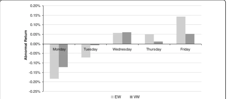
Figure 1 presents the average abnormal return of the EW and VW portfolios on each day of the week in the 1953–2006 period, where average abnormal return is defined as the average return of a portfolio on a particular day minus the average return across all week days for that portfolio. Figure 1 shows a pattern of improv-ing returns in the EW portfolio. However, the pattern is disrupted by the fact that Wednesday’s average abnormal return is larger than Thursday’s. In the VW portfo-lio, the disruption is even larger since Wednesday’s return is larger than both Thursday’s and Friday’s.

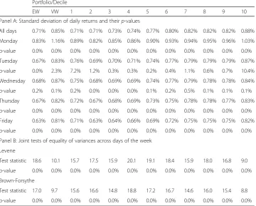
Before we turn to analyzing the average abnormal returns, it is important to de-termine whether returns across days of the week are homoscedastic. The existing evidence suggests that return variances across days of the week are not homosce-dastic (e.g., Aggarwal and Schatzberg, 1997; Connolly, 1989). Panel A of Table 1 provides information on the standard deviations of daily returns from Monday to Friday across the various deciles and portfolios. The evidence in Table 1, Panel A, suggests substantial variation in the standard deviations across days of the week, with Mondays exhibiting the highest standard deviations and Fridays the lowest.

Using a chi-square distribution Panel A of Table 1 also reports p-values for the null hypothesis σ2

ij¼σ2i, where σ2ij is the variance of portfolioion dayjand σ2i is the vari-ance of portfolioiacross all days. The evidence in Table 1, Panel A, strongly rejects the null hypothesis that the variance of a particular day is equal to the variance of all week-days, except for two cases: deciles 1 and 10 on Tuesday (for which the p-values are 7.2% and 10.4%, respectively).

Panel B of Table 1 provides results of the Levene (1960) and Brown-Forsythe (1974) tests for the joint null hypothesis that variances across days of the week are all equal. The results of these tests strongly reject the hypothesis of homoscedastic-ity, as p-values are practically zero in all cases. Following the evidence provided in Table 1, our analysis proceeds under the assumption of heteroscedasticity.

Table 2 reports statistical analysis of the daily abnormal returns across days of the week in the full 1953–2006 period. Table 2, Panel A, presents the results for single-day

-0.25% -0.20% -0.15% -0.10% -0.05% 0.00% 0.05% 0.10% 0.15% 0.20%

Monday Tuesday Wednesday Thursday Friday

A

bnor

ma

l R

e

tu

rn

EW VW

(4)

average abnormal returns and their respective p-values. The null hypothesis in these tests isμ_ij= 0, whereμ_ijis the average abnormal return for portfolio i on day j. The re-sults in Table 2, Panel A, show a pattern of improving returns during the week in dec-iles 1 through 4. In decdec-iles 5 through 9, and in the EW portfolio, the pattern of improving returns is disrupted, however, by the fact that Wednesday’s average abnor-mal return is higher than Thursday’s. In decile 10, and in the VW portfolio, the viola-tion of the pattern is even larger since Wednesday’s average abnormal return is larger than that of Thursday’s and Friday’s. The results in Table 1, Panel A, also show that the statistical significance of the single-day average abnormal daily return is impressive – the average abnormal return is statistically significant in all cases but two (decile 10 on Tuesday and Thursday).

Panel B of Table 2 provides results for the joint hypothesis that average abnormal returns are equal across all days of the week. The tests that are used for this purpose are standard analysis of variance (ANOVA) and ANOVA adjusted for heteroscedasticity (Welch 1951). The results show that the null hypothesis – that average abnormal returns are equal across all days of the week – is strongly rejected as all p-values in Panel B of Table 2 (both the homoscedasticity and heteroscedasticity cases) are close to zero.

Table 1Are variances equal across days of the week?

Portfolio/Decile

EW VW 1 2 3 4 5 6 7 8 9 10

Panel A: Standard deviation of daily returns and theirp-values

All days 0.71% 0.85% 0.71% 0.71% 0.73% 0.74% 0.77% 0.80% 0.82% 0.82% 0.82% 0.88% Monday 0.83% 1.16% 0.89% 0.82% 0.85% 0.86% 0.90% 0.93% 0.94% 0.95% 0.96% 1.03% p-value 0.0% 0.0% 0.0% 0.0% 0.0% 0.0% 0.0% 0.0% 0.0% 0.0% 0.0% 0.0% Tuesday 0.67% 0.83% 0.76% 0.69% 0.70% 0.71% 0.74% 0.77% 0.79% 0.79% 0.79% 0.87% p-value 0.0% 2.3% 7.2% 1.2% 0.3% 0.3% 0.2% 0.4% 1.1% 0.6% 0.7% 10.4% Wednesday 0.68% 0.87% 0.75% 0.68% 0.69% 0.69% 0.74% 0.77% 0.79% 0.78% 0.78% 0.84% p-value 0.2% 0.1% 0.2% 0.0% 0.0% 0.0% 0.1% 0.2% 0.5% 0.1% 0.1% 0.1% Thursday 0.67% 0.82% 0.72% 0.67% 0.68% 0.69% 0.73% 0.75% 0.78% 0.78% 0.77% 0.83% p-value 0.0% 0.0% 0.0% 0.0% 0.0% 0.0% 0.0% 0.0% 0.0% 0.0% 0.0% 0.0% Friday 0.63% 0.81% 0.71% 0.63% 0.64% 0.66% 0.69% 0.72% 0.75% 0.75% 0.75% 0.82% p-value 0.0% 0.0% 0.0% 0.0% 0.0% 0.0% 0.0% 0.0% 0.0% 0.0% 0.0% 0.0% Panel B: Joint tests of equality of variances across days of the week

Levene

Test statistic 18.6 10.1 15.7 17.5 15.9 20.1 19.1 18.4 15.9 18.0 16.8 9.0 p-value 0.0% 0.0% 0.0% 0.0% 0.0% 0.0% 0.0% 0.0% 0.0% 0.0% 0.0% 0.0% Brown-Forsythe

Test statistic 17.0 9.7 15.6 16.6 14.8 18.8 17.2 16.7 14.6 16.0 15.4 8.8 p-value 0.0% 0.0% 0.0% 0.0% 0.0% 0.0% 0.0% 0.0% 0.0% 0.0% 0.0% 0.0%

Table 1 provides information on standard deviations of returns across days of the week for the EW, VW, and size decile portfolios in the 1953–2006 period. Panel A provides the standard deviation for the relevant day and portfolio/decile, and the corresponding p-value for the null hypothesisσ2

ij¼σ2i, whereσ2ijis the variance of portfolio i on day j andσ2iis

the variance of portfolio i across all days of the week. The results in Panel A suggest substantial variation in the variances across days of the week, with Monday displaying the highest variance and Friday the lowest. Panel B provides the results of two statistical tests, the Levene and Brown-Forsythe tests, for the more general null hypothesisσ2

i;Mon¼σ2i;Tue¼σ2i;Wed

¼σ2

i;Thu¼σ2i;Fri¼σ2i. The results in Panel B suggest that the null hypothesis of homoscedasticity is rejected for

(5)

(6)

The evolution of the day-of-the-week effect

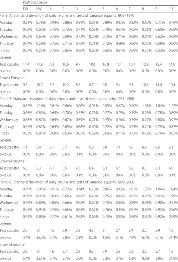
In this section, we analyze the evolution of the day-of-the-week effect in three 18-year subperiods: 1953–1970, 1971–1988, and 1989–2006. The purpose of this analysis is to examine the evolution of the day-of-the-week effect over time. Figure 2 displays the average abnormal returns for the EW and VW portfolios across days of the week in the three subperiods.

We begin the subperiod analysis by testing for heteroscedasticity in the three subpe-riods. The results of the heteroscedasticity tests are reported in Table 3.

The results in Table 3 indicate that heteroscedasticity is present in the large majority of the cases. The sizes of the F-statistics suggest, however, a decline in the magnitude of heteroscedasticity to the degree that, in terms of statistical significance, heterosce-dasticity has disappeared in some of the largest capitalization deciles during the recent 1989–2006 period. Nevertheless, the bulk of the evidence in Table 3 rejects the null

-0.25% -0.20% -0.15% -0.10% -0.05% 0.00% 0.05% 0.10% 0.15% 0.20%

A

b

no

rm

al

R

et

ur

n

1953–1970

EW VW

-0.25% -0.20% -0.15% -0.10% -0.05% 0.00% 0.05% 0.10% 0.15% 0.20%

A

b

no

rm

al

R

et

ur

n

1971–1988

EW VW

-0.25% -0.20% -0.15% -0.10% -0.05% 0.00% 0.05% 0.10% 0.15% 0.20%

A

b

no

rm

al

R

et

ur

n

1989–2006

EW VW

(7)

Table 3Are variances equal across days of the week? Subperiod analysis

Portfolio/Decile

EW VW 1 2 3 4 5 6 7 8 9 10

Panel A: Standard deviation of daily returns and tests of variance equality 1953_–1970

Monday 0.81% 0.78% 0.94% 0.88% 0.89% 0.87% 0.89% 0.87% 0.82% 0.80% 0.77% 0.79% Tuesday 0.62% 0.65% 0.75% 0.72% 0.71% 0.68% 0.70% 0.67% 0.65% 0.61% 0.60% 0.68% Wednesday 0.65% 0.65% 0.75% 0.69% 0.71% 0.70% 0.73% 0.71% 0.68% 0.64% 0.62% 0.68% Thursday 0.64% 0.59% 0.75% 0.71% 0.72% 0.71% 0.72% 0.69% 0.66% 0.62% 0.59% 0.60% Friday 0.57% 0.55% 0.75% 0.65% 0.66% 0.63% 0.65% 0.61% 0.59% 0.55% 0.53% 0.56% Levene

Test statistic 11.4 11.8 6.3 10.6 9.7 10.1 10.8 11.1 10.7 12.9 12.4 11.0 p-value 0.0% 0.0% 0.0% 0.0% 0.0% 0.0% 0.0% 0.0% 0.0% 0.0% 0.0% 0.0% Brown-Forsythe

Test statistic 9.5 10.7 6.2 10.2 8.5 8.7 9.0 9.3 9.3 10.6 11.0 10.4 p-value 0.0% 0.0% 0.0% 0.0% 0.0% 0.0% 0.0% 0.0% 0.0% 0.0% 0.0% 0.0% Panel B: Standard deviation of daily returns and tests of variance equality 1971–1988

Test statistic 7.1 5.4 6.1 5.7 4.8 6.6 6.8 7.3 6.5 8.9 6.6 5.1

p-value 0.0% 0.0% 0.0% 0.0% 0.1% 0.0% 0.0% 0.0% 0.0% 0.0% 0.0% 0.0% Brown-Forsythe

Test statistic 6.8 5.3 6.1 5.5 4.5 6.4 6.3 6.7 6.2 8.3 6.3 4.9

p-value 0.0% 0.0% 0.0% 0.0% 0.1% 0.0% 0.0% 0.0% 0.0% 0.0% 0.0% 0.1% Panel C: Standard deviation of daily returns and tests of variance equality 1989–2006

Test statistic 2.5 1.1 4.5 2.9 2.8 4.3 3.1 2.7 2.4 2.2 2.9 1.2

p-value 4.4% 35.2% 0.1% 2.0% 2.3% 0.2% 1.5% 3.1% 4.9% 6.7% 2.1% 31.4% Brown-Forsythe

Test statistic 2.3 1.1 4.6 2.7 2.8 4.3 2.9 2.6 2.2 2.0 2.7 1.2

p-value 5.4% 35.1% 0.1% 2.7% 2.6% 0.2% 2.3% 3.7% 6.3% 8.8% 3.0% 31.8%

(8)

hypothesis of homoscedasticity, and therefore the subperiod analysis below proceeds under the assumption of heteroscedasticity.

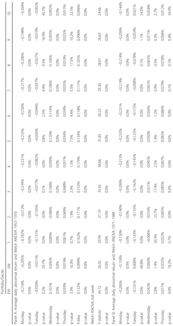
Table 4 reports the analysis of the daily abnormal returns in the three subperiods. Table 4, Panel A, reports the results for the first subperiod; Table 4, Panel B, reports re-sults for the second subperiod; and Table 4, Panel C, reports rere-sults for the third sub-period. The first part in each panel reports the average abnormal returns and their statistical significance, and the second part reports results for the Welch ANOVA.

Examination of the average abnormal returns in Table 4 suggests that the pattern of improving returns throughout the week is also present in the subperiods. However, as in the full-period analysis, Wednesday’s return seems too high and violates the pattern in many cases.

The results in Table 4 also suggest that the magnitude of the day-of-the-week effect has declined over time. This can be observed in the size of the F-statistics in the EW and VW portfolios. In the VW portfolio, the F-statistic is 26.92 in the first subperiod, 6.51 in the second subperiod, and 0.30 in the third subperiod. In the EW portfolio, the F-statistics are 34.72, 37.25, and 15.00, respectively. Hence, although not entirely smooth in the EW portfolio, there is a general tendency of decline in the magnitude of the day-of-the-week effect. Note also that, as part of this decline, the effect disappeared in the last subperiod in the largest capitalization decile (decile 10) and in the VW port-folio. In decile 9, the effect became borderline significant. The effect remains, however, statistically significant in all other 8 deciles and in the EW portfolio in the last subpe-riod. Consistent with other studies, we conclude that these results show a decline in the magnitude of the effect over time (see, for example, Brusa et al. 2000; Gu 2004; Kohers et al. 2004; Mehdian and Perry 2001; Kamara 1997). The evidence, however, does not suggest that the effect has vanished.

Conclusion

We study the day-of-the-week effect across size deciles and over time. Full period ana-lysis (1953–2006) of the day-of-the-week effect shows that returns are monotonically increasing during the week in the four smallest capitalization deciles.

However, the pattern of increasing returns is interrupted in the EW and size deciles 5 through 9 by the fact that Wednesday’s average abnormal return is higher than Thurs-day’s. In decile 10 and in the VW portfolio, the interruption of the pattern is even larger since Wednesday’s average abnormal return is larger than that of both Thursday’s and Friday’s.

The behavioral explanation of the day-of-the-week effect is based on empirical find-ings that mood tends to improve throughout the week. Thus, if the behavioral explan-ation is true, we should expect returns to improve throughout the week. Our evidence thus suggests that the behavioral hypothesis is a stronger candidate in the smaller capitalization deciles.

(9)

(10)

(11)

Endnotes 1

See, for example, Gibbons and Hess (1981), Keim and Stambaugh (1984), Lako-nishok and Smidt (1988), Abraham and Ikenberry (1994), Aggarwal and Schatzberg (1997), Pettengill (2003).

2

See, for example, Liano and Lindley (1995), Kohers and Kohers (1995), Keim and Stambaugh (1984), Gibbons and Hess (1981).

Acknowledgements

I thank Gady Jacoby for many suggestions and comments.

Funding

Not applicable

Author’s information

Shlomo Zilca is an independent researcher. He holds Ph.D. in finance from Tel Aviv University. Shlomo taught statistics and investments at the University of Auckland and Tel Aviv University.

Competing interests

The author declares that he has no competing interests.

Publisher’s Note

Springer Nature remains neutral with regard to jurisdictional claims in published maps and institutional affiliations.

Received: 6 October 2017 Accepted: 1 November 2017

References

Abraham A, Ikenberry D (1994) The individual investor and the weekend effect. J Financ Quant Anal 29:263_–277 Aggarwal R, Schatzberg JD (1997) Day-of-the-week effects, information seasonality, and higher moments of security

returns. J Econ Bus 49:1_–20

Bader AM (2005) Relationship between depression and anxiety among undergraduate students in eighteen Arab countries: a cross-cultural study. Soc Behav Pers 33:503_–512

Birru J (2017) Day-of-the-week and the cross section of returns. Working paper, fisher College of Business, the Ohio State University

Brockman P, Michayluk D (1998) Individual versus institutional investors and the weekend effect. J Econ Financ 22:71– 85

Brooks RM, Kim H (1997) The individual investor and the weekend effect: a reexamination with intraday data. Q Rev Econ Finance 37:725_–737

Brown MB, Forsythe AB (1974) Robust tests for the equality of variances. J Am Stat Assoc 69:364–367

Brusa J, Liu P, Schulman C (2000) The weekend effect,_‘reverse_’weekend effect, and firm size. J Bus Finance Account 27: 555–574

Chang E, Pinegar J (1998) US day-of-the-week effects and asymmetric responses to macroeconomic news. J Bank Finance 22:513–534

Chen H, Singal V (2003) Role of speculative short sales in price formation: the case of the weekend effect. J Financ 58: 685–705

Cole DA, Peeke LG, Lachlan G, Martin JM, Truglio R, Seroczynski AD (1998) A longitudinal look at the relation between depression and anxiety in children and adolescents. J Consult Clin Psychol 66:451–460

Connolly R (1989) An examination of the robustness of the weekend effect. J Financ Quant Anal 24:133_–170 Cross F (1973) The behavior of stock prices on Fridays and Mondays. Financ Anal J 29:67–69

Damodaran A (1989) The weekend effect in information releases: a study of earnings and dividend announcements. Rev Financ Stud 2:607–623

DeFusco R, McCabe G, Yook K (1993) Day-of-the-week effects: a test of information timing hypothesis. J Bus Finance Account 20:835–842

Dyl E, Maberly E (1988) A possible explanation of the weekend effect. Financ Anal J 44:83_–84

Farber M (1953) Time-perspective and feeling-tone: a study in the perception of the days. J Psychol 35:253–257 Fields M (1931) Stock prices: a problem in verification. J Bus 4:415_–418

Fishe R, Gosnell T, Lasser D (1993) Good news, bad news, volume and the Monday effect. J Bus Finance Account 20: 881_–892

French K (1980) Stock returns and the weekend effect. J Financ Econ 8:55–69 Gibbons M, Hess P (1981) Day-of-the-week effects and asset returns. J Bus 54:579_–596

Golder SA, Macy MW (2011) Diurnal and seasonal mood vary with work, sleep, and daylength across diverse cultures. Science 333:1878_–1881

Gondhalekar V, Mehdian S (2003) The blue-Monday hypothesis: evidence based on Nasdaq stocks, 1971–2000. Q J Bus Econ 42:73_–92

(12)

Hirshleifer DA, Jiang D, Meng Y (2017) Mood beta and seasonalities in stock returns. Working paper, SSRN library, abstract 2880257

Jacobs B, Levy K (1988) Calendar anomalies: abnormal returns at calendar turning points. Financ Anal J 44:28–39 Kamara A (1997) New evidence on the Monday seasonal in stock returns. J Bus 70:63–84

Keim D, Stambaugh R (1984) A further investigation of the weekend effect in stock returns. J Financ 39:819–835 Kelly F (1930) Why you win or lose: the psychology of speculation. Houghton Mifflin, Boston

Kohers T, Kohers G (1995) The impact of firm size differences on the day-of-the-week effect: a comparison of major stock exchanges. Appl Financ Econ 5:151–160

Kohers G, Kohers N, Pandy V, Kohers T (2004) The disappearing day-of-the-week effect in the World’s largest equity markets. Appl Econ Lett 11:167–171

Lakonishok J, Maberly E (1990) The weekend effect: trading patterns of individual and institutional investors. J Financ 45:231–243

Lakonishok J, Smidt S (1988) Are seasonal anomalies real? A ninety year perspective. Rev Financ Stud 1:403–425 Levene H (1960) Robust tests for the equality of variances. In: Olkin I, Ghurye SG, Hoeffding W, Madow WG, Mann HB

(eds) Contribution to probability and statistics. Stanford University Press, Palo Alto CA

Liano K, Lindley J (1995) An analysis of the weekend effect within the monthly effect. Rev Quant Finan Acc 5:419–426 Markese J (1989) Stock market anomalies: folklore that may not be myth. Am Assoc Individ Investors 11:30–33 Mehdian S, Perry M (2001) The reversal of the Monday effect: new Evidence from US equity markets. J Bus Finance

Account 28:1043–1065

Pettengill G (1993) An experimental study of the‘blue Monday’hypothesis. J Socioecon 22:241–257

Pettengill G (2003) A survey of the Monday effect literature. Quarterly Journal of Business and Economics 42:3–27 Pettengill G, Buster D (1994) Variations in return signs: announcements and the weekday anomaly. Quarterly Journal of

Business and Economics 33:81–91