PhD Dissertation
International Doctorate School in Information and Communication Technologies
DIT - University of Trento
Techniques for robust source separation and localization in
adverse environments
Issues and performance of a new framework of emerging techniques for frequency-domain convolutive blind/semi-blind separation and localization of acoustic sources
Francesco Nesta
Advisor:
Prof. Maurizio Omologo
FBK-irst Fondazione Bruno Kessler
Acknowledgment
Abstract
Acoustic source separation is a relatively recent topic of signal processing which aims to simul-taneously separate many acoustic sources recorded through one or more microphones. Such a problem was formulated to emulate the natural capability of the human auditory system which is able to recognize and enhance the sound coming from a particular source. Addressing this problem is of high interest in the automatic speech recognition (ASR) community since it would improve the effectiveness of a natural human-machine interaction. Among numerous methods of multichannel blind source separation techniques, those based on the Independent Compo-nent Analysis (ICA) applied in the frequency-domain [81] are the most investigated, due to their straightforward physical interpretation and computational efficiency. In spite of recent developments many issues still need to be address to make such techniques robust in adverse conditions, such as high reverberation, ill-conditioning and occurrence of permutations. Fur-thermore, most of the proposed BSS methods are computationally expensive and not feasible for a real-time implementation.
This PhD thesis describes a research activity in the robust separation of acoustic sources in adverse environment. A new framework of blind and semi-blind techniques is proposed which allows source localization and separation even in highly reverberant environment and with real-time constraint. For each proposed technique, theoretical and practical issues are discussed and a comparison with alternative state-of-art methods is provided. Furthermore, the robustness of the proposed framework is validated implementing two real-time blind and semi-blind systems which are tested in challenging real-world scenarios.
Contents
1 Introduction 1
1.1 The Problem of Source Enhancement . . . 1
1.2 Multichannel Source Enhancement . . . 3
1.2.1 Model . . . 4
1.2.2 Fixed Beamformers . . . 5
1.2.3 Adaptive Beamformers . . . 6
1.3 Scope and Thesis Outline . . . 8
1.4 Publications . . . 10
1.4.1 International Journal Publications . . . 10
1.4.2 International Conference Publications . . . 10
2 An introduction to BSS 13 2.1 Instantaneous Linear Model . . . 15
2.1.1 Principal Component Analysis . . . 16
2.1.2 Independent Component Analysis . . . 17
2.1.3 ICA Based on Nongaussianity . . . 20
2.2 NG and KL divergence . . . 21
2.3 BSS for convolutive mixtures . . . 23
2.3.1 Main framework for convolutive BSS . . . 24
3 Frequency-Domain BSS 31 3.0.2 Output Source Estimation . . . 32
3.0.3 Scaling Ambiguity and Minimal Distortion Principle (MDP) . . . 33
3.0.4 Circularity of FFT . . . 35
3.1 Permutation Problem . . . 36
3.2 Physical Interpretation of FD-BSS . . . 37
4.2 RR-ICA . . . 45
4.2.1 Wiener-like weighting . . . 45
4.2.2 Relationship between Wiener-like weighted ICA and Adaptive Beam-Formers . . . 47
4.2.3 Least Mean Square tracking of the demixing matrix . . . 48
4.2.4 Proposed algorithm . . . 49
4.2.5 RR-ICA and Others BSS . . . 50
4.3 Experimental results . . . 51
4.3.1 Experiments with simulated data . . . 52
4.3.2 Experiments with real-world data . . . 56
4.4 Concluding Remarks . . . 59
4.5 Appendix . . . 60
5 GSCT 65 5.1 Introduction . . . 65
5.2 FD-BSS and ideal acoustic propagation . . . 66
5.3 State Coherence Transform . . . 69
5.3.1 Equivalence Between SCT and MLE . . . 70
5.3.2 Equivalence Between SCT and Kernel pdf Estimation . . . 72
5.3.3 Definition ofg(·)and Adaptive Estimation ofα . . . 74
5.3.4 Connections Between SCT and GCC-PHAT . . . 76
5.3.5 Numerical Evaluation of the SCT . . . 78
5.4 Generalized State Coherence Transform . . . 79
5.4.1 Numerical Evaluation . . . 82
5.4.2 GSCT and Computational Issues . . . 83
5.5 Solving Real-World problems with the SCT/GSCT . . . 85
5.5.1 Spatial Localization of Multiple Sources; . . . 85
5.5.2 Reduction of Permutations . . . 92
5.5.3 Underdetermined Source Separation by Spatial Filtering . . . 101
5.6 Concluding Remarks . . . 103
6 cSPEC 105 6.1 Introduction . . . 105
6.2 Limitation of SCT and Permutation Problem . . . 106
6.3 Correlation-based Approaches and Their Limitations . . . 107
6.5 Proposed Algorithm . . . 111
6.6 Experimental Results . . . 112
6.7 Concluding Remarks . . . 114
7 SBSS applied to MCAEC 115 7.1 Introduction . . . 115
7.2 A review of the LMS algorithm . . . 117
7.3 Theoretical analysis of SBSS . . . 121
7.3.1 Model . . . 121
7.3.2 Non-Uniqueness Problem . . . 124
7.3.3 Steady-State Solution forH12b . . . 125
7.3.4 Connection between MSE and ICA . . . 128
7.3.5 Effect of Constraint onW(ω) . . . 129
7.4 Algorithmic design and related issues . . . 132
7.4.1 Online Implementation of SBSS . . . 132
7.4.2 Proposed SBSS Algorithm . . . 135
7.5 Experimental evaluation . . . 137
7.5.1 Evaluation Methods . . . 137
7.5.2 Experimental Results . . . 138
7.6 Appendix . . . 151
7.7 Concluding Remarks . . . 151
8 Towards Distributed BSS 153 8.1 Introduction . . . 153
8.2 BSS as Soft-Masks Estimation . . . 154
8.3 Cooperative Wiener-ICA . . . 156
8.4 Experimental Results . . . 158
8.5 Concluding Remarks . . . 160
9 Real-time BSS/SBSS 161 9.1 Introduction . . . 161
9.2 Architecture of the BSS system . . . 161
9.2.1 Input processing . . . 163
9.2.2 ICA-BSS (first-stage) . . . 164
9.2.3 SCT . . . 164
9.2.4 ICA-BSS (second stage) . . . 164
9.2.5 Output processing . . . 165
9.4.2 ICA-SBSS . . . 178
9.4.3 Output processing . . . 179
9.4.4 BSS . . . 179
9.4.5 Start-end point detector . . . 181
9.4.6 ASR . . . 181
9.5 Evaluation of the SBSS algorithm . . . 182
10 Conclusions 187
List of Tables
5.1 µP(σP)in%with known TDOAs . . . 98
5.2 µP(σP)in%with SCT . . . 99
5.3 µP(σP)in%forT60= 150 msandd= 0.1 m . . . 101
7.1 Outline of the proposed SBSS algorithm. . . 135
7.2 Procedure for adaptation of the de-mixing matrix. . . 136
7.3 Summary of parameters used during adaptation. . . 138
8.1 Pseudo code description of the Cooperative Wiener ICA. . . 157
List of Figures
1.1 Example of cocktail party problem . . . 2
1.2 Typical scenarion for a speech controlled system in presence of background interfering noise and loudspeaker echos . . . 3
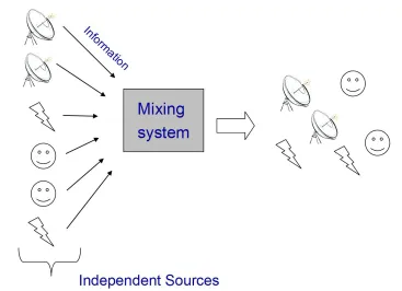
2.1 Generic mixing model for a source separation system . . . 14
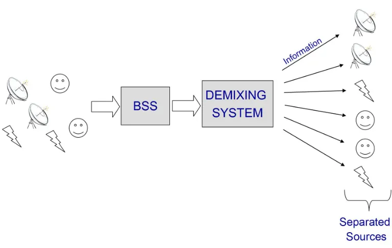
2.2 Generic demixing model for a source separation system . . . 15
2.3 Example of ICA applied to EEG . . . 18
2.4 Example of ICA applied to image separation . . . 18
2.5 IVA mixing model for the case of 2 sources and 2 microphones[45]. . . 26
3.1 Cost function computed for the case of two sources . . . 40
4.1 Magnitude of the determinant ofW(k)andWtracked(k)across frequencies. . . 50
4.2 Graphical representation of the relationship between the degree of freedom of the solution and the BSS approaches. . . 51
4.3 Simulated test setup, for a room characterized byT60= 300ms. . . 52
4.4 PME between the estimated and true propagation models. The ICA is applied to signal segments of just 1 second and with different number of ICA iterations. 54 4.5 PME between the estimated and true propagation models. The Scaled NG is applied to signal segments of just 1 second. The performance is compared applying jointy or individually the two proposed regularization strategies. . . . 55
4.6 Graphical representation of the relationship between number of ICA iterations and the type of knowledge which defines the final solution. . . 55
4.7 Block diagram of the implemented BSS algorithm. . . 56
lengths. . . 58
4.10 Results obtained in the Test2 experiments. Best performance is reported in terms of SIR and SDR, by applying the given algorithms with different signal lengths. . . 58
4.11 Average performance computed from all the possible combinations of FFT size and signal length. . . 58
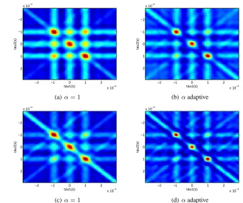
5.1 Simulated time-delay distribution and estimated SCT with fixed α for three source located at−20◦,0◦ and20◦. . . . 79
5.2 Simulated TDOA distribution and estimated SCT with adaptedαfor three source located at−20◦,0◦ and20◦. . . . . 79
5.3 Original time-delay distributions . . . 81
5.4 GSCT computed according to different vector metrics. Case with microphone distanced= 0.01 . . . 83
5.5 GSCT computed according to different vector metrics. Case with microphone distanced= 0.1 . . . 84
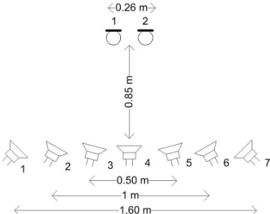
5.6 Experimental setup for the case of 7 sources. . . 87
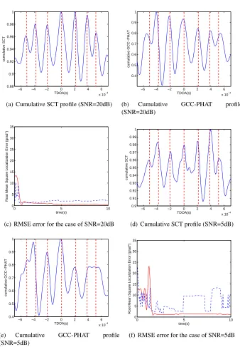
5.7 Comparison between the cSCT and the cumulative GCC-PHAT. The red dotted lines are the true expected TDOAs. (c) and (f) show the RMSE localization error for the cumulative GCC-PHAT (blue dotted line) and the cSCT (solid red line) . . . 88
5.8 Selected TDOAs from the estimated cumulative SCT (the red dotted lines are the true expected TDOAs). . . 89
5.9 Comparison between the SCT and the cumulative GCC-PHAT for 4 sources recorded with microphones spaced of0.05m. In the envelopes the red dotted lines are the true expected TDOAs. In (c) is plotted the RMSE localization error for the cumulative GCC-PHAT (blue dotted line) and the SCT (solid red line) . 89 5.10 Comparison between the cumulative SCT and the cumulative GCC-PHAT. In the envelopes the red dotted lines are the true expected TDOAs. In (c) and (f) is plotted the RMSE localization error for the cumulative GCC-PHAT (blue dotted line) and the cumulative SCT (solid red line) . . . 90
5.11 Approximated GSCT and cumulative SCT over the dimensionτ1 andτ2 . . . . 91
5.12 Configuration of the simulated setup (T60 = 300ms) . . . 92
5.13 GSCT map computed over the7×7TDOA pairs . . . 92
5.14 GSCT map . . . 93
5.16 Permutation map forT60= 150 ms,d= 0.02 m . . . 96
5.17 Permutation map with known TDOAs . . . 97
5.18 Histograms ofP, known TDOAs,T60 = 300 ms . . . 98
5.19 Permutation error across frequency,T60= 150 ms . . . 99
5.20 Permutation map for SCT . . . 100
5.21 Histogram ofP with SCT,T60= 300 ms . . . 100
5.22 Perm. error across frequency,T60= 150 ms,d= 0.1 m . . . 101
5.23 Recording setup for undetermined source separation . . . 103
5.24 Performance undetermined separationT60 = 150ms . . . 103
5.25 Performance undetermined separationT60 = 300ms . . . 104
6.1 Polar diagram of the phase ofrik. . . 108
6.2 Typical spectrogram of an bad permuted output source . . . 110
6.3 Permutation errors for TDOA and cSPEC alignment. . . 112
6.4 Convergence curve of the permutation errors. . . 113
6.5 Performance evaluation. . . 113
7.1 Model per a single-channel AEC system . . . 118
7.2 Model for stereophonic acoustic echo cancellation (SAEC). . . 120
7.3 Model of the near-end and the far-end mixing systems and the semi-blind source separation (SBSS) system. . . 121
7.4 Source activities in the worst-case scenario. . . 139
7.5 Performance of SBSS after using AWGN to decorrelate the reference signals (with de-mixing matrix constraints and 5 iterations). . . 141
7.6 Performance of constrained and unconstrained SBSS (with 5 iterations). . . 141
7.7 Performance of SBSS with different number of iterations (with de-mixing ma-trix constraint). . . 142
7.8 Performance of SBSS with different EBR (with de-mixing matrix constraint and 5 iterations). . . 143
7.9 Performance of SBSS against AWGN noise at near-end microphones (with de-mixing matrix constraint and 5 iterations). . . 143
7.10 Performance of SBSS against reverberation time T60 (with de-mixing matrix constraint and 5 iterations). . . 144
7.11 Performance of SBSS for different FFT frame size (with de-mixing matrix con-straint and 5 iterations). . . 144
7.14 Performance of SBSS against variation of the active source number (with
de-mixing matrix constraint and 5 iterations). . . 147
7.15 Performance of SBSS for different microphone configurations (with de-mixing matrix constraint and 5 iterations). . . 147
7.16 Performance of SBSS for different microphone configurations without applying the near-end source separation (with de-mixing matrix constraint and 5 iterations).148 7.17 Comparison between SBSS and FBNLMS for a real-world scenario . . . 150
7.18 Comparison between SBSS and FBNLMS for a real-world scenario in the ideal case of no near-end sources . . . 150
8.1 Interconnection of the network by a token ring topology. . . 157
8.2 Experimental setup. . . 158
8.3 Performance comparison for different inter-microphones and inter-pair spacing. 158 8.4 Source location likelihood obtained by means of the GSCT computed with the statesrnk; states obtained by independent unconstrained ICA adaptations (case a), and states obtained by CW-ICA adaptations (case b). . . 159
9.1 Logical architecture of the developed BSS system. . . 162
9.2 Hardware architecture of the developed BSS system. . . 162
9.3 Frequency response and directivity pattern of the AKG C400 BL (from the orig-inal specification datasheet). . . 163
9.4 Description of the input processing stage. . . 163
9.5 Description of the first ICA stage for the BSS. . . 164
9.6 Description of the permutation correction stage based on the SCT . . . 165
9.7 Description of the second ICA stage. . . 165
9.8 Description of the output processing stage for BSS. . . 166
9.9 Setup of the source locations. . . 167
9.10 Explanation of the dynamic conditions generated in Task1. . . 168
9.11 Explanation of the dynamic conditions generated in Task2. . . 169
9.12 State-machine for the detection of the number of active sources . . . 169
9.13 Frequency response of the A-weighting filter. . . 170
9.14 Task1, pdf of the SIR performance computed without A-weighting filter. . . 171
9.15 Task1, pdf of the SDR performance computed without A-weighting filter. . . . 171
9.16 Task1, pdf of the SIR performance computed with A-weighting filter. . . 172
9.17 Task1, pdf of the SDR performance computed with A-weighting filter. . . 172
9.19 Task2, pdf of the SDR performance computed without A-weighting filter. . . . 174
9.20 Task2, pdf of the SIR performance computed with A-weighting filter. . . 174
9.21 Task2, pdf of the SDR performance computed with A-weighting filter. . . 175
9.22 Task2, SIR performance envelope computed without A-weighting filter. . . 175
9.23 Task2, SDR performance envelope computed without A-weighting filter. . . 176
9.24 Task2, SIR performance envelope computed with A-weighting filter. . . 176
9.25 Task2, SDR performance envelope computed with A-weighting filter. . . 177
9.26 Logical architecture of the developed SBSS system. . . 177
9.27 Hardware architecture of the developed SBSS system. . . 177
9.28 Description of the input processing stage for the SBSS. . . 179
9.29 Description of the ICA stage for the SBSS. . . 180
9.30 Description of the output processing stage for the SBSS. . . 180
9.31 Block description of the start-end point detector. . . 181
9.32 Block description of the ASR module. . . 182
9.33 Setup for the SBSS evaluation . . . 182
Chapter 1
Introduction
1.1 The Problem of Source Enhancement
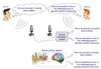
Sound source enhancement is a relatively recent topic of signal processing which aims to sim-ulate the natural capability of the human auditory system to extract a sound source of interest from a complex noisy auditory scene. Human brain is successfully able to perform this task every day and this capability allows people to hold a conversation even in a noisy environment like that of a ”Cocktail party”. The solution to the so called ”cocktail party problem” is one of the challenging goals of acoustic research community and gives rise to a lot of interest. The emulation of the human capability is an essential step towards a new generation of machines which are able to naturally interact with humans. In our society, such an interaction have been increasing due to the wide spread of information technologies. In fact, the way human beings live has been drastically changing due to the increasing importance of the information exchange in the everyday life.
Nowadays, the interaction is still oriented to a computer perspective and does not use the same methods naturally adopted by humans to interact with the environment. An important evolution to reduce the gap between machines and humans is making the interaction as natural as possible. One important step to reach this goal is to build systems, which are able to inter-act with people using verbal communication. Much progress has been achieved in the speech processing community, which made it possible to build real-life applications, based on human-machine speech interactions. For instance, dictating into favorite word processing application, asking for information in a museum, controlling device without usage of hands, writing notes on a mobile phone, finding paths in big cities while driving, etc. These applications are possible with the progress of speech recognition and synthesis technologies.
Figure 1.1: Example of cocktail party problem
interfering sources, such as music, vehicular noise or speech of other humans. It is clear that techniques of source enhancement become essential to make the overall goal achievable. In general source enhancement can be achieved by segregating a real-world sound mixture in their basic individual components. For the human auditory system addressing this task is rela-tively easy in spite of the few sensors (i.e. two ears) used to sense the environment. On the other hand, the robustness of artificial systems is more sensitive to the quantity of recorded data. In the last two decades promising results have been obtained in the solution of the ”cocktail party problem” by means of statistical methods under the name of blind source separation (BSS). Such techniques aim to separate and extract sources of interest with only a small knowledge on their statistical properties [72] and differ from previous methods for their high efficiency and applicability to real-life problem. In general BSS methods can be classified in two main categories:
• single channel methods; • multi channel methods.
CHAPTER 1. INTRODUCTION 1.2. MULTICHANNEL SOURCE ENHANCEMENT
Figure 1.2: Typical scenarion for a speech controlled system in presence of background interfering noise and loudspeaker echos
the most popular techniques on which many methods have been formulated. However, their applicability to real-life problems is still limited due to the poor robustness and performance, if a good prior knowledge on the target properties is not available. Furthermore, the high compu-tational complexity hampers the adoption of these algorithms for real-time application. On the other hand, multi-channel BSS is the most robust one since it uses geometrical knowledge on the acoustic scene. Recent progress in the field indicates that those techniques can be applied to real-world problems with real-time constraints [57][2]. For such a reason, these techniques form the basis of this thesis work which will be presented in the next sections.
1.2 Multichannel Source Enhancement
Beamformers generally require a high number of sensors to obtain gain pattern with an acceptable spatial rejection of the interfering sources from the target source. More important, they need to be supervised by other techniques for source localization and activity detection. On the other hand, blind source separation methods do not require additional information more than the knowledge of the statistical characterization of the sources. However, BSS methods based on sensor array exploit the same spatial redundancy to perform the source separation and can be considered a class of unsupervised beamformers. For such reasons in the next section a brief introduction on the fundamentals of beamforming techniques is given since it is essential for the BSS methods which will be presented in the next chapters.
1.2.1 Model
Let us consider a time-domain signal recorded in open field condition by the sensors of the array x(t) = [x1(t), x2(t), ..., xM(t)]T and for sake of simplicity let us assume to have in the auditory scene one narrow-band source which can be modeled as:
s(t) =ksin(2πf t) (1.1)
wherek is the amplitude andf is the carrier frequency. In complex-domain the source can be represented as:
s(t) =kej2πf t (1.2)
The signals recorded by the array can be considered as delayed and scaled versions of the orginal source signals.
x(t) =
x1(t) · · ·
xM(t)
=
α0ks(t−T0) · · ·
αM−1ks(t−TM−1)
=kej2πf t
α0e−j2πf T0 · · ·
αM−1e−j2πf TM−1
(1.3)
Note that the attenuation αm only depends on the distance between the microphone and the source if we ideally assume each microphone having unitary gain. Assuming to be in far-field condition and the array to have linear geometry with uniform microphone spacing (Uniform Linear Array) the time of arrivals Tm−1 between the source and the m-thmicrophone can be expressed as:
Tm−1 =T0+ ∆tm−1 =T0+m
dcosθ
c , ∀m >1 (1.4)
whered is the microphone spacing,θ is the Direction Of the Arrival of the source (DOA) and
CHAPTER 1. INTRODUCTION 1.2. MULTICHANNEL SOURCE ENHANCEMENT
rewritten as:
x(t) =x1
1 · · · ˆ
αM−1e−j2πf∆TM−1
'x1
1
· · ·
e−j2πf(M−1)dcosθ c
=x1a(f, θ) (1.5)
whereαˆm is the attenuation ratio αm = ααm0 (which in far-field is approximated to 1for each
m). The vectora(f, θ)is defined as steering vector of the ULA array for a source located at the angleθ. The goal of a beamformer is to estimate a row vector of coefficientsw(f)so that the output signalw(f)x(t)is an estimate of the original sources(t):
y(t) =x1(t)w(f)a(f, θ) = x1(t)b(f, θ)'s(t) (1.6)
whereb(f, θ)indicates the transfer function between a source at locationθand the beamformer output. The squared magnitude ofb(f, θ)defines the beampattern which indicates the gain of the global transfer function of the beamformer in a given directionθ.
Ifs(t)is a broadband source the signal recorded at each microphone can be considered the convolution of the source and the impulse response between source and microphones:
x(t) =
x1(t) · · ·
xM(t)
=
s(t)∗h1(t) · · ·
s(t)∗hM(t)
. (1.7)
Here∗indicates the convolution operator. There are generally two methods of beamforming. One is to deconvolvex(t)by an FIR filter of lengthLwhich approximate the inverse response
hmfor each sensor and to form the output by summing over each contribution. Alternatively the beamforming can be applied in frequency domain by transforming the signal x(t) in narrow-band signalsx(f, t) (i.e. by means of band pass filtering or short-time Fourier analysis) and applying beamforming techniques for narrow-band sources. In this work we will focus on frequency-domain approaches since it is the same used for the BSS methods proposed in the next chapters.
1.2.2 Fixed Beamformers
obtained deterministically as:
wm(f) =
1
Me
j2πf c−1(m−1)dcos(θ)
(1.8)
Assuming to have an ideal knowledge of the DOAθthe performance of a fixed delay-and-sum beamformer depends on the microphone distance and on the wave length of each narrow-band source. It is interesting to plot for each frequency thebeampatternof a beamformer steered in a given direction θ1. It is clearly observed that the resolution of the beamformer and the gain attenuation in each direction is not constant. Therefore, applying narrow-band techniques to broadband sources would result in a non uniform attenuation of the interfering sources across the frequencies. In particular the residual of the interfering source would sound as its low-passed filtered since the spatial attenuation increases with the frequencies.
A simple approach to impose a constant directivity is to perform a least-square optimization of the coefficients in order to impose the average pattern across frequencies to have a given shape.
w(f) = argmin
w(f)
Z
|b(θ)−w(f)a(f, θ)|2dθ (1.9)
where b(θ)is the desidered frequency-invariant response. One major drawback of delay-and-sum beamformer is the low directivity which is approximatively proportional to the number of microphones. It has been found that the directivity of linear endfire arrays theoretically approachesM2as the spacing approach to0in isotropic noise [92]. This capability is exploited by superdirective beamformerswhere the filters w(f)are optimized in order to maximize the factor of directivity (or array gain).
Fixed beamformers are easy to implement and do not introduce any computational load since the coefficients can be predetermined for some directionsθ and switched according to the location of the sources. As major drawback their effectiveness is strictly dependent on the number of sensors and on their calibration. In fact a pre-calibration procedure is essential to compensate the variation on the gain of the microphones (theoretically assumed to be equal to1) and to have an exact geometrical knowledge of the array. Therefore, fixed-beamformers are very sensitive to calibration errors which make the resulting beampatterndifferent from the true optimal one.
1.2.3 Adaptive Beamformers
To overcome the limitations of fixed-beamformers adaptive weight estimation is generally pre-ferred. While common fixed beamformers enhance a target sound coming from a given direction by forming directional beampatterns, Adaptive BeamFormers (ABF) estimate the weightsw(f)
CHAPTER 1. INTRODUCTION 1.2. MULTICHANNEL SOURCE ENHANCEMENT
aims to reduce the energy of the acoustic wave, impinging to the array, related to the interfering sources. We briefly review this technique since it was shown that under certain conditions it is strictly connected with the frequency-domain BSS [4].
From now on we represent the signals in frequency-domain. Let us consider the vector the sourcess(f) = [s1(f), s1(f),· · · , sN(f)]T. The signals recorded at each microphone are modeled as:
x(f) = H(f)s(f) (1.10) where the generic elementhmn(f) of the matrixH(f)is the frequency response between the m-thmicrophone andn-thsource. An estimation of the signalss(f)can be obtained by means of a demixing matrixW(f):
y(f) = W(f)x(f). (1.11) Assumings1(f) to be the source of interest and theN −1remaining sources to be the inter-ferences, the enhancement can be achieved by the determining the weights which ensure the following equivalence:
w1(f)hn(f) = 0, ∀n = 2,· · · , N (1.12)
wherew1(f)andhn(f)are the sub vectors defined as:
w1 = [w11(f), w12(f),· · · , w1M(f)], hn(f) = [h1n(f), h2n(f),· · · , hM n(f)]T (1.13)
Ideally, the resulting output signals would be equivalent to:
y1(f) =w1(f)x(f)'w1(f)h1(f)s1(f) (1.14)
The mixing coefficient hn(f) are not known in advanced and the weights w1(f) need to be adaptively estimated. If the target source is not active, the weights can be adapted in order to minimize the output energy:
w1(f) = argmin w1(f)
E[|w1(f)x(f)|2] (1.15)
can rewrite the optimization rule as:
w1(f) = argmin w1(f)
h|w1(f)x(f, t)|2it∈T (1.16)
where h·it is time-averaging operator and T is the time subset for which s1 is inactive. The optimization in (1.16) has a degenerate solution forw1(f)which is that to set all the elements equal to 0. Therefore to prevent such degeneration we need to constrain the optimization in order to keep invariant the energy coming from the target source. A common way is to impose the following constraint:
w1(f)a(f, θ) = 1 (1.17)
where a(f, θ1) is the steering vector of the array for the source s1(f) (located in θ1). If the source is in far-field for an ULA the vector a(f, θ1)can be defined as in (1.5). Note in (1.5), in far-field the relative attenuationαˆm is approximated to 1but the direction of arrivalθ needs to be known or estimated in advance. Finally, the solution which optimizes (1.16) under the constraint (1.17) is obtained as:
w1(f) =
a(f, θ1)HR−1(f) a(f, θ1)HR−1(f)a(f, θ1)
(1.18)
whereR(f)is the covariance matrix of the recorded signalsx(f, t):
R(f) = hx(f, t)x(f, t)Hi
t∈T (1.19)
An adaptive beamformer ideally defines an upper bound on the performance of a multichannel source separation system [5] since it directly attempts to minimize the output energy of an in-terfering source. However, its optimality is subject to the condition that the target source is not continuously active in order that the adaptation based on the optimization rule in (1.15) is mean-ingful. When the locations and the activity of the sources is not known, ABF are inappropriate and BSS techniques must be considered.
1.3 Scope and Thesis Outline
CHAPTER 1. INTRODUCTION 1.3. SCOPE AND THESIS OUTLINE
• high reverberation • real-time feasibility
• multiple source localization in multiple dimensions • separation of short mixtures
• robust solution to the permutation problem of frequency-domain BSS • extension to semi-blind case
• applicability of BSS to distributed array networks The thesis is organized as follows:
• chapter 2 recalls the fundamentals of the Blind Source Separation problem and of the Independent Component Analysis (ICA). Moreover, it focuses on the separation of con-volutive mixtures of acoustic sources and on its state-of-art.
• chapter 3 gives a deep description of the frequency-domain BSS and of the related issues. • chapter 4 proposes an extension of the traditional ICA based frequency-domain BSS to
overcome its limitation when short signals are processed.
• chapter 5 proposes the Generalized State Coherence Transform (GSCT). The GSCT is a multidimensional spatial likelihood function which exploits the phase coherence of demixing matrices estimated by an ICA algorithm, in order to evaluate the parameters of the wave propagation of acoustic sources. The GSCT is a useful tool to allow source separation and localization of acoustic sources.
• chapter 6 discusses and proposes a new method based on a coherent source spectral esti-mation for solving the permutation problem of frequency-domain blind source separation (BSS).
• chapter 7 discusses the problem of Semi-blind source separation (SBSS) which is a special case of the blind source separation when some partial knowledge of the source signals is available to the system. Theoretical and practical issues are deeply analyzed and an SBSS algorithm is proposed and evaluated.
• chapter 8 discusses and evaluates in a preliminary analysis a new scheme, under the name of Collaborative Wiener ICA, to perform the BSS using distributed arrays.
1.4 Publications
1.4.1 International Journal Publications
• Francesco Nesta, Piergiorgio Svaizer, Maurizio Omologo, ”Convolutive BSS by recur-sively regularized ICA across frequencies” (accepted for publication in the IEEE Trans-actions in Audio Speech and Language processing)
• Francesco Nesta, Ted Wada, Biing-Hwang (Fred) Juang, ”Batch-Online Semi-Blind Source Separation Applied to Multi-Channel Acoustic Echo Cancellation” (accepted for publication in the IEEE Transactions in Audio Speech and Language processing) • Francesco Nesta, Maurizio Omologo, ”Estimation of the multidimensional acoustic
propagation parameters of multiple sources with the Generalized State Coherence Transform” (in preparation for submission to IEEE Transactions in Audio Speech and Language processing).
1.4.2 International Conference Publications
• Francesco Nesta, Maurizio Omologo, ”Cooperative Wiener-ICA for source localization and separation by distributed microphone arrays”, (in proceedings) ICASSP2010 • Benedikt Loesch, Francesco Nesta, and Bin Yang, ”On the robustness of the
mul-tidimensional State Coherence Transform for solving the permutation problem of frequency-domain ICA, (in proceedings) ICASSP2010
• Francesco Nesta, Ted Wada, Shigeki Miyabe, Biing-Hwang (Fred) Juang, ”On the non-uniqueness problem and the semi-blind source separation”, (in proceedings), WAS-PAA 2009
• Francesco Nesta, Maurizio Omologo ”Generalized State Coherence Transform for multidimensional localization of multiple sources”, (in proceedings), WASPAA 2009 • Francesco Nesta, Ted Wada, Biing-Hwang (Fred) Juang, ”Coherent spectra estimation
for a robust solution to the permutation problem”, (in proceedings) to WASPAA 2009 • Francesco Nesta, Piergiorgio Svaizer, and Maurizio Omologo, ”Cumulative State Co-herence Transform for a Robust Two-Channel Multiple Source Localization”, (in proceedings), ICA 2009
CHAPTER 1. INTRODUCTION 1.4. PUBLICATIONS
• Francesco Nesta, Maurizio Omologo, Piergiorgio Svaizer, ”Multiple TDOA estimation by using a state coherence transform for solving the permutation problem in frequency-domain BSS”, (in proceedings), MLSP 2008
• Francesco Nesta, Maurizio Omologo, Piergiorgio Svaizer, ”A novel robust solution to the permutation problem based on a joint multiple TDOA estimation”, (in proceed-ings), IWAENC 2008
• Francesco Nesta, Piergiorgio Svaizer, Maurizio Omologo, ”Separating short signals in highly reverberant envirnonment by a recursive frequency-domain BSS”, (in pro-ceedings), HSCMA 2008
Chapter 2
An Introduction to Blind Source
Separation
Blind Source Separation (BSS) is a relatively recent digital signal processing technique that has given rise to a lot of interest in the last two decades [72]. Its main objective is to separate multiple sources mixed through unknown channels using only the observations of their mix-tures. Such techniques have been applied in many scientific fields such as biology, biomedical signal processing, digital communication and speech processing. The term “blind” indicates that separation is performed without using any information about the mixing channels or the sources.
Let us consider a set ofN sourcess(t) = [s1(t), s2(t),· · · , sN(t)]T and a set ofM mixture observationsx(t) = [x1(t), x2(t),· · · , xM(t)]T obtained as:
x(t) =H[s(t)] +e(t) (2.1)
whereH[·] is a generic transfer function and e(t)is a column vector of additive noise terms. AssumingH[·]invertible the goal of a Source Separation system is to estimate a functionW[·]
in order to reconstruct the original source signalss(t):
y(t) = W[x(t) +e(t)] (2.2)
Figure 2.1: Generic mixing model for a source separation system
well as to the characteristic of the sources. The complexity of a BSS system strictly depends on the model used to represent the generic transfer function. For the case of acoustic sources two main models give rise of interest:
• instantaneous mixing model • anechoic mixing model • convolutive mixing model
The simplest case of BSS regards the separation of instantaneous mixtures when the observed signals are linear combinations of the original source signals. To a large extent, this case is solved by means of the Independent Component Analysis (ICA)[38]. The goal of the ICA methods is to find a representation of nongaussian data so that the estimated components are as statistically independent as possible.
CHAPTER 2. AN INTRODUCTION TO BSS 2.1. INSTANTANEOUS LINEAR MODEL
Figure 2.2: Generic demixing model for a source separation system
A more challenging case regards sources which are mixed through convolutive channels. This situation is quite common for audio applications where signals are generally recorded in rever-berant environments.
In the next sections we discuss the instantaneous model and the basis of the ICA theory. After that we consider the convolutive model, treating the anechoic one as a special case.
2.1 Instantaneous Linear Model
The simplest way to model the observed signals is to assumex(t)to be a vector of instantaneous linear mixtures of the source signals:
x(t) = Hs(t) (2.3)
whereHis the mixing matrix which is assumed for simplicity to be time-invariant. Assuming the number of the mixture observations to be greater than the number of the sources (M ≥N) the problem is defined asoverdeterminated (orovercomplete) and the original sources can be retrieved by estimating the pseudo inverse ofH:
which for the case of N =M is equivalent to the inverse ofH. Therefore the original signals are demixed as:
y(t) =Wx(t) (2.5)
If N > M, known asunderdeterminated case, the matrix HTH is not fully ranked and thus a pseudo inverse of W does not exit. Therefore, the estimation of the output signals cannot be addressed by linear demixing of the observations vector even though theoretically it is still possible to estimate a mixing matrixH.
2.1.1 Principal Component Analysis
The Principal Component Analysis (PCA), often named Karhunen-Lo´eve transform, is a well-known statistical tool used to reduce the representation of a signal by means of a set of variables with less redundancy [37]. The method is based on Second-Order Statistic (SOS) and has the main goal to represent the observed data series with uncorrelated series. Assumingx(t)to be a set of zero-mean random variables we can define the autocorrelation matrix as:
Rxx =E[xxH] (2.6)
where we removed the time dependency to simplify the notation. The PCA decomposition associated withxis defined as:
Rxx =QDQH (2.7)
where D is a diagonal matrix whose elements dii are the principal eigenvalues of Rxx corre-sponding to the eigenvectors Q = [q1,q2, ...]. Thus, the principal components ofx(t)can be obtained by the whitening transformation:
V =√DQH (2.8)
z(t) =Vx(t) (2.9)
Multiplying the elements ofx(t)byQH the outputs would represent an orthogonal base, while the term√Dnormalizes the variance of the signals which become also orthonormal.
Note that if the signalsx(t)are obtained as in (2.3),z(t)do not necessarily correspond to the original components s(t) since uncorrelatedness corresponds to independence only if the sources s(t) are normally distributed. Furthermore, it is possible to demonstrate that only by means of SOS correlation the identification of W is not possible. For example, if the sources s(t)are mutually independent their covariance matrix is diagonal:
CHAPTER 2. AN INTRODUCTION TO BSS 2.1. INSTANTANEOUS LINEAR MODEL
whereDsis a generic diagonal matrix. For the goal of the source separation we want to estimate a demixing matrixW in order to recover the original components s. According to SOS the matrixWmust decorrelate the estimated output signalsy(t):
arg
W
(E[WxxHWH] =D
s) (2.11)
which can be rewritten as:
arg
W
(E[WHssHHHWH] =D
s) (2.12)
arg
W
(WHDs(WH)H =Ds) (2.13)
Assuming for simplicity that the sources have unitary autocorrelation,Ds is equivalent to the identity matrixIand the matrixU=WHis unitary:
arg
W
(UUH =I) (2.14)
IfW and Hdo not have a particular structure the matrix Wcan only be determined up to a unitary transformationU:
W=UH+ (2.15)
where+is the Moonre-Penrose pseudo inverse. Therefore the uncorrelatedness is only a nec-essarily but not sufficient condition for independence and therefore cannot be used to separate stationary sources mixed through a linear mixing system. Nevertheless, the whitening proce-dure is widely used in many High-Order-Statistics (HOS) methods as preprocessing tool to limit the search of the solution in a bounded space, consequently increasing the convergence rate and the adaptation stability.
2.1.2 Independent Component Analysis
Figure 2.3: Example of ICA applied to EEG
Figure 2.4: Example of ICA applied to image separation
to a number of scientific fields such as astronomic image analysis [31][51], biomedical signal separation [56][79] and video coding [77],[69]. The scope of this thesis is to provide a set of robust methods for acoustic source separation in convolutive adverse environments based on ICA. The proposed methods do not require a deep knowledge of the huge mathematical for-mulations of ICA theory which goes behind the scope of this thesis. Therefore, we limit the discussion only to the fundamentals of the ICA and we give a description of the Natural Gradi-ent algorithm which is on the bases of the methods proposes in the next chapters.
Two main hypotheses need to be verified to successfully apply the ICA:
• The source signals need to be mutual independent which means that, for continuous vari-able, the joint probability density function of the sourcess(t)can be marginalized as:
p(s1, s2,· · · , sN) =p(s1)p(s2)· · ·p(sN) (2.16)
An equivalent way to express such an independence is by means of high order cross mo-ments. Considering a set of time-domain signals s(t) = [s1(t)...sN(t)] we can define withSi(t)the random variable associated to the source signal observed at time instantt. Sources are assumed independent if the following relationship holds:
E[Sn1(t)
αS
n2(t−τ)
β] = 0 ∀n
CHAPTER 2. AN INTRODUCTION TO BSS 2.1. INSTANTANEOUS LINEAR MODEL
situation for acoustic sources such as speech and music.
• According to the PCA analysis, stationary sources cannot be separated only by means of second-order-statistics. Therefore, if the sources have a Gaussian distribution all the high-order moments are null and thus the separation is neither possible by means of ICA. In general it is required that at most one source can have Gaussian statistics if we want to uniquely identify an inverse of the mixing matrixH[28].
The first assumption is probably the biggest limitation of ICA. In fact, though independent sources are expected to generate uncorrelated signals, the HOS independence has sense only if evaluated over a sufficient data observations (theoretically infinite). However, in practical situation the estimation of the mixing system is performed with a limited amount of data which may correspond to highly correlated signal sources. Therefore, the high statistical bias in the evaluation of the HOS could compromise the accuracy of the solution if the observed data is not sufficiently large.
As for the PCA also the ICA solution has some ambiguities:
• scaling ambiguity (or variance indeterminacy). From equation (2.3) we note that since boths(t)andHare unknown, any scalar multiplier in one of the sourcessn(t)could be always cancelled by dividing the corresponding n-th column of H by the same scalar. Therefore, if one of the variables, H or s(t) is unknown, it is not possible to retrieve the correct variance of the original sources. Note that the scalar can also be negative and therefore there is also an ambiguity of sign. One of the methods used to solve this problem is to impose the variance of sources to be unitary. However, we will see later that for the frequency-domain convolutive BSS a better method is used to reduce the spectral distortion in the output signals.
• order ambiguity (or permutation indeterminacy). Still, since the structure of the mixing matrix His unknown one could freely invert the order of the rows of W (which would correspond to change the order of the column of H) still obtaining at output indepen-dent signals. This ambiguity is well-known as permutation indeterminacy. In other terms, given a demixing matrixWfor any permutation matrixΠ, the resulting permuted demix-ing matrixΠWis still a solution.
To summarize the above indeterminacies, we can say that the separation matrixW estimated by the ICA is an estimate of the inverseHup to a scaling and permutation ambiguity:
W=ΛΠH−1 (2.18)
2.1.3 ICA Based on Nongaussianity
As already mentioned one of the cues used in ICA is that signal have nongaussian statistics. According to the Central Limit Theorem (CLT) the distribution of a sum of independent random variables tends toward a normal distribution. If an observed signal is a mixtures of two or more independent signal sources its distribution is expected to be more Gaussian than that of each single source. Thus, one criteria to estimate W is to maximize the non-gaussianity of the output signals distributions.
W=argmax
˜ W
Ng[ ˜Wx(t)] (2.19)
whereNg[·]indicates a function which measures the nongaussianity of the output signals. Givensbeing a zero-mean random variable a classical measure of nongaussianity is the kurtosis or the fourth-order cumulant defined as:
kurt(s) = E[s4]−3E[s2]2 (2.20)
which is generally simplified withE[s4]−3if the variable is normalized to unit variance. The kurtosis is 0if sis Gaussian, while assumes negative and positive values for subgaussian and supergaussian distribution, respectively. Subgaussian distributions have typically a flat pdf (i.e. uniform distribution). On the other hand, supergaussian distribution have aspikyor heavy tailed pdf; an important example is the Laplace distribution defined as:
p(s) = √1
2e
√
2|s| (2.21)
Laplace pdf is widely use to model the distribution of acoustic sources in frequency-domain. Acoustic sources such as speech or music have a sparse representation in time-frequency do-main which means that the signals assume values close to zero in most of the time-frequency points. Therefore an effective method to extract a speech from a mixture of signals is by max-imizing the supergaussianity of the output signalsy, which means to increase their sparseness in time-frequency domain.
The kurtosis is an interesting function since it is easy to compute and have linear properties which simplify the formulation of adaptation methods:
kurt(s1+s2) =kurt(s1) +kurt(s2) (2.22)
CHAPTER 2. AN INTRODUCTION TO BSS 2.2. NG AND KL DIVERGENCE
Typically, sources are separated by means of the kurtosis applying a deflation procedure which extracts sequentially the sources with the highest kurtosis [21]. However, the kurtosis is not a robust measure since it is high sensitive to outliers [87]. For this reason other mea-sures of non-gaussianity have been proposed. An information theoretic quantity to measure the nongaussianity is given by the negentropy which is based on the entropyH(·)defined as:
H(s) =−
Z
pdf(s)log[pdf(s)]ds (2.24)
wheresis a vector of random variables. The entropy of a random variable represents the degree of information given by their observations. It is well-known that among the distributions with the same variance, a Gaussian random variable is that with the highest entropy or in other terms that with the lowest information. Therefore a measure of non gaussianity may be performed by defining the negentropyJ as:
J(s) =H(sg)−H(s) (2.25) where sg is a vector of random variables of the same covariance matrix of s. The practical evaluation of the negentropy is not an easy task since there is not any closed form to evaluate the entropyH. Therefore approximation are generally made as:
J(s)'(E[G(v)]−E[G(s)])2 (2.26)
where v is a standardized Gaussian variable and G is some nonquadratic contrast function. Many contrast functions have been proposed which increase the robustness of the negentropy when compared to kurtosis based measures [39]. A popular method which uses the approxima-tion in (2.26) is the popular Fast-ICA algorithm [40].
2.2 Natural Gradient and Kullback-Liebler Divergence
A popular method proposed in [3] is to estimate W by minimizing the mutual dependence between the sources according to a Natural Gradient optimization. It was shown in [38] that the minimization of the mutual dependence is connected to the Infomax principle which is a popular method for BSS based on the maximization of the output entropy of a neural network with non-linear outputs [8]. Furthermore it was shown in [13] that under certain conditions the Infomax principle is connected to the maximum-likelihood estimation ofW proposed in [14] and [20].
observationsMand the sources are mutually independent with zero mean. For the basic deriva-tion of the Natural gradient it is also assumed that the noisee(t)is negligible but extensions to the noisy case are provided by other methods such as Robust ICA [18].
The statistical independence between the output sources can be achieved by minimizing dif-ferent statistical measures of mutual dependence. A popular method is to derive an adaptive learning rule which minimizes the Kullback-Leibler divergence between the joint probability distribution of the output sources p(y(t))and the product of the marginal probability distribu-tionsQNn=1p(yn(t)), which is defined for the output sourcesy(t)as:
IKL =
Z
p(y(t))logQNp(y(t))
n=1p(yn(t))
dy(t) (2.27)
After some mathematical manipulation, (2.27) can be rewritten as:
IKL 'E[logp(y(t))]−E
"
N
X
n=1
logp(yn(t))
#
(2.28)
whereE[·]is the expectation operator.
By means of the steepest descent gradient the matrix Wis updated in the direction which minimizes ∂IKL
∂W . The derivation of the gradient can be split considering separately the two terms in the equation (2.28). Applying the partial derivative to the first term in the RHS of the equation leads to:
∂E[logp(y(t))]
∂W =
∂ ∂WE
·
log p(x(t)) |det(W)|
¸
=−∂E[log|det(W)|]
∂W =−E[W
−1]T (2.29) whereT is the matrix transpose. Deriving the partial derivative of each term in the summation of the second term of equation (2.28) leads to:
∂E[logp(yn(t))]
∂Wnm
=E
" ∂p(yn(t))
∂yn(t)
p(yn(t))
∂yn(t)
∂Wnm
#
=E
" ∂p(yn(t))
∂yn(t)
p(yn(t))
xm(t)
#
(2.30)
The pdf derivative cannot be analytically derived but it can be approximated as: ∂p(yn(t))
∂yn(t)
p(yn(t))
' −φ(yn) (2.31)
CHAPTER 2. AN INTRODUCTION TO BSS 2.3. BSS FOR CONVOLUTIVE MIXTURES
be represented by the same model) we define the non-linearity vector functionΦas:
Φ(y(t)) = [φ(y1(t)),· · · , φ(yN(t))]T (2.32)
Therefore the gradient can be approximated to:
∂IKL
∂W =−E[W
−1]T +E[Φ(y(t))y(t)T] (2.33) The gradient−∂IKL
∂W represents the steepest decreasing direction of functionIKL when the pa-rameter space is Euclidean. In our case the separation is possible only if the matrixW is not singular and therefore the space of the solutions is represented by all theN ×N non singular matricesW[18]. By means of such an evidence in [3] it was introduced a Riemannian metric to the space ofW. It was shown that the true steepest-descent direction in the Riemannian space of parameters is−∂IKL
∂W WTW. Finally the adaptive learning rule takes the following form: W←−W+η(I−E[Φ(y(t))y(t)T])W, y(t) =Wx(t) (2.34)
The matrixΦ(y(t))y(t)T is known as generalized covariance matrixand is expected to be di-agonal if the output signals are mutual independent. If the demixing matrix W is estimated on-line with the incoming datax(t), the expectation of the gradient is substituted with its in-stantaneous value. On the other hand, if the learning is applied to a batch of observed datay(t), the expectation may be substituted with the average over time.
2.3 BSS for convolutive mixtures
The linear model is rarely useful for the separation of acoustic sources in real environment. In fact, the mixing system is not well represented by a simple linear mixing model. In indoor environments, microphones record many replicas of the same acoustic source which propagate according to the different reflection paths and thus reach the array with different time-delays. Therefore, a better model for the recorded signals is to consider the mixtures x(t)as sum of convolved version of the original sourcess(t)according to the impulse response between each source and microphone.
x(t) = h(t)∗s(t) (2.35) where∗indicates the convolution operator andh(t)is the matrix of the impulse responses:
h(t) =
h11(t) · · · h1N(t) · · · · · · · · ·
hM1(t) · · · hM N(t)
IfM ≥N the output signals would be estimated as:
y(t) = w(t)∗x(t)'s(t) (2.37)
wherew(t)is a matrix of deconvolution filters:
w(t) =
w11(t) · · · w1N(t) · · · · · · · · ·
wM1(t) · · · wM N(t)
(2.38)
In a practical implementation of a convolutive BSS, the demixing filters w(t)are discrete and have a finite length L which needs to be chosen according to the reverberation time of the room and to the frequency fs used to sample the signals x(t). The number of parameters that need to be estimated is M × N × L and thus the complexity increases with the length of the demixing filters needed to compensate the impulse responses. Therefore, the formulation of BSS algorithm for convolutive mixtures is much more complex than that of instantaneous mixtures since many parameters need to be jointly optimized by the same adaptation. Such a complexity represents also an obstacle to robustness of convolutive time-domain BSS since its convergence behavior becomes more unstable asLincreases due to the sensitivity of gradient-based adaptation to the presence of local minima.
2.3.1 Main framework for convolutive BSS
Defining the state-of-art for the convolutive blind source separation field is not a trivial oper-ation. In fact in the last decade a lot of ideas have been proposed but there is not a common evaluation framework that would allow one to have a clear comparison between the methods. Some trials to define an objective comparison have been done in the last two SIgnal source Sep-aration Evaluation Campaigns (SISEC, [95]). However, a the lack of an objective evaluation criteria, coherent with the quality perceived by human listeners, hampered a clear interpretation of the results. Moreover, the optimality of the separation have been often overstressed against the robustness among environmental conditions, which would have a stronger impact in real-world applications. Furthermore, there is still a number of theoretical limits that still must be addressed and no method is able to address the source separation for all the cases. In this the-sis, rather than defining the state-of-art for the convolutive BSS, we preferred to select three main BSS frameworks which, according to the author, are the most interesting according to the following evaluation criteria:
CHAPTER 2. AN INTRODUCTION TO BSS 2.3. BSS FOR CONVOLUTIVE MIXTURES
• capability to solve the separation for challenging situations
• innovation of the proposed work.
The chosen methods are: 1) Independent Vector Analysis 2) TRINICON (”Triple-N ICA for convolutive mixtures”) 3) Frequency-domain BSS based on ICA. In the next subsections we briefly recall the bases of the first two methods while we will deeply analyze the third one in a separated chapter, since it defines the starting point for the innovative methods proposed in this thesis work.
IVA: Independent Vector Analysis
The Independent Vector Analysis is a recent method proposed by Intae Lee et al. [45] which aims to extend the ICA to the multivariate case. According to the property of the Fourier transform convolutive mixtures of time-domain signals can be represented by instantaneous mixture in frequency domain. This property is exploited by methods of BSS which perform the source separation in frequency-domain. However, applying the separation to each frequency independently the permutation problem [81] must be solved, which means find for the optimal permutation of the output at each frequency in order to group together all the components related to the same source. Especially in highly reverberant environment and when we work with a lot of sources the solution to the permutation problem is not trivial. The Independent Vector Analysis introduces a frequency coupling directly in the adaptive learning rule, in order to reduce the occurrence of wrong permutations.
Compared with ICA which works with uni-variate components signals, IVA extends the separation to multivariate components. The signal statistics is modeled with a multivariate distribution which consider all the frequencies at the same time. The adaptive optimization aims to find the set of the demixing matrices which makes the output multivariate signals as much independent as possible. Since all the frequency components are considered at the same time, the output source dependencies are minimized with correct permutations of the demixing matrices across the frequencies. Therefore, inner dependency between frequency components of each output are intrinsically considered. IVA is equivalent to a multiple layers of standard ICA where the demixing matrix of all the frequencies are jointly optimized. Figure 2.5 shows the mixing model for a generic case ofN sources andM microphones. Each original source is modeled as a multivariate component assn =
h
s1
n, s2n, ... sKn
iT
whereKis the number of the frequency components according to the short-time Fourier transform analysis. Similarly, the observed mixtures are modeled as: x1 =
h
x1
m, x2m, ... xKm
iT
Figure 2.5: IVA mixing model for the case of 2 sources and 2 microphones[45].
output source asyn =
h
y1
n, y2n, ... ynK
iT
where each component is estimated as:
ynk =
M
X
m=1
wnmk xkm, (2.39)
where wk
nm are the coefficients of the demixing matrix Wk which separates the components of the k-th frequency. IVA aims to estimate the demixing matrices Wk which minimizes the mutual dependence between the output sources. Similarly to ICA an adaptive learning rule can be derived in order to minimize the Kullback-Leibler divergence between the joint probability distribution of the output sources p(y1,· · · ,yN) and the product of approximated marginal probability distributionq(yn):
C =KL
Ã
p(y1,· · · ,yN)|| N
Y
n=1
q(yn)
!
(2.40)
After some mathematical manipulation (2.40) can be rewritten as:
C =const+
F
X
f=1
log|det(W−1 d )| −
X
n
CHAPTER 2. AN INTRODUCTION TO BSS 2.3. BSS FOR CONVOLUTIVE MIXTURES
whereW−1
d is the inverse estimate ofAdandE[·]is the expectation operator. Note that in this case the marginal probability distribution ofyn is a multivariate distribution of his K compo-nents. By differentiating the cost functionC with respect to the coefficientswk
nmand according to the Natural Gradient rule we obtain the following adaptation:
W(ki+1) =W(ki)+η(I−E[Φk(y1,· · · ,yK)yH k])W
(i)
k (2.42)
whereiis the index of the iteration, yH
k is the Hermitian transpose ofykandΦk(y1,· · · ,yK) is a vector of contrast function of all the output componentsyk
n. Defining the density model of
q(yn)as a scale mixture of Gaussian distributions, the elements of the vector approximates to:
φk
n(yn1,· · · , yKn) =
yn
qPK
k=1|ynk|
(2.43)
The IVA algorithm has been applied to some challenging situations. The reported performance are very interesting and show that using constraints that introduce frequency dependence is a good strategy to improve the standard frequency-domain approach. However, the intrinsic com-plexity due to the high dimensionality of the contrast function slow-down the convergence of the algorithm and the computational cost is still too expensive to be implemented in real-time. Fur-thermore, similarly to time-domain methods the IVA updates all the variables within the same adaptation and is highly sensitive to the convergence into local minima. This drawback results in a high instability which lowers the average separation performance even when compared with tradition frequency-domain methods. A better discussion of such a problem is discussed in the next sections where the IVA has been used as a comparison algorithm for many experiments on simulated and real-world data.
TRINICON Blind Source Separation
The TRINICON based BSS is an alternative approach to perform the separation in time-domain. The framework presented by Buchner et al. [12] introduces a new model to deal with both blind source separation and multichannel blind deconvolution (MCBD). Multivariate models are used in the cost function to consider the entire temporal structure of the original source signals. The structure is analyzed by a block processing which is a simplification of the optimal formulation for the BSS in time-domain. The observed signals are segmented in blocks of lengthLB. Each sample in time-domain is modeled asx(b, shif t)whereb is the the block index and shif t is the time-shift index within the block, which can assume value from0toLB−1. The separated signals are modeled as:
The vectors are composed byN elements according to the number of the sources (assumed to be equal to the number of microphonesM).
x(b, shif t) = h
x1(b, shif t), · · · , xM(b, shif t)
i
(2.45)
y(b, shif t) = h
y1(b, shif t), · · · , yN(b, shif t)
i
(2.46) The separation matrix for a given block can be represented as:
W(b) =
W11(b), · · · ,W1M(b) ... . .. ... WN1(b), · · · ,WNM(b)
(2.47)
Them-thmixture is modeled as:
xm(b, shif t) =
h
xm(bL+shif t), · · · , xM(bL−2L+ 1 +shif t)
i
(2.48)
where L is the length of the FIR filters used to model the mixing system. At same way the output signals are modeled as:
yr(b, shif t) = h
yn(bL+shif t), · · · , yN(bL−D+ 1 +shif t)
i =
M
X
m=1
xm(b, shif t)Wmn(b) (2.49)
whereDis the number of the time-lags taken into account to exploit the non-whiteness of the source signals. EachWnm(b)is a Sylvester2L×Dmatrix which contains the filter coefficients of the deconvolution filters between then-thsource and them-thmicrophone. The TRINICON method aims to estimate the demixing matrices Wnm(b) which are an exact estimate of the inverse of eachHmn(b)in order to have a perfect separation and deconvolution of the sources:
C=Hnm(b)Wmn(b) =I, ∀n, m, b (2.50)
The demixing matrix in TRINICON is estimated according to three different optimization cri-teria:
1. Nongaussianity: already used by ICA methods that aim to minimize the mutual depen-dence of the outputs.
CHAPTER 2. AN INTRODUCTION TO BSS 2.3. BSS FOR CONVOLUTIVE MIXTURES
different time-instants.
According to these criteria a general cost function and an optimization rule are defined. The TRINICON framework is versatile since it realizes an estimation of the demixing system with a straightforward physical interpretation of the problem, according to the model of the mixing sys-tem in time-domain. Theoretically, the framework can be applied to any number of sources and for any reverberation time. However, increasing the length of the deconvolution filters the num-ber of the parameters that have to be estimated is too high. To make possible the separation in a real-time context some approximations have been implemented, mainly based on the Second Order Statistics (SOS). These approximations introduce further reduction to the convergence speed and robustness of the algorithm and limit the possibility to apply the TRINICON-BSS in a real adverse conditions.
Frequency-Domain BSS based on ICA
Chapter 3
Frequency-Domain BSS
A popular method to simplify the BSS for real-world scenario is to decompose the convolutive BSS into independent simpler tasks by transforming th