Robust PCA by Manifold Optimization
Teng Zhang [email protected]
Department of Mathematics University of Central Florida 4000 Central Florida Blvd Orlando, FL 32816, USA
Yi Yang [email protected]
Department of Mathematics and Statistics McGill University
805 Sherbrooke Street West Montreal, QC H3A0B9, Canada
Editor:Michael Mahoney
Abstract
Robust PCA is a widely used statistical procedure to recover an underlying low-rank matrix with grossly corrupted observations. This work considers the problem of robust PCA as a nonconvex optimization problem on the manifold of low-rank matrices and proposes two algorithms based on manifold optimization. It is shown that, with a properly designed initialization, the proposed algorithms are guaranteed to converge to the underlying low-rank matrix linearly. Compared with a previous work based on the factorization of low-low-rank matrices Yi et al. (2016), the proposed algorithms reduce the dependence on the condition number of the underlying low-rank matrix theoretically. Simulations and real data examples confirm the competitive performance of our method.
Keywords: principal component analysis, low-rank modeling, manifold of low-rank matri-ces.
1. Introduction
In many problems, the underlying data matrix is assumed to be approximately low-rank. Examples include problems in computer vision Epstein et al. (1995); Ho et al. (2003), machine learning Deerwester et al. (1990), and bioinformatics Price et al. (2006). For such problems, principal component analysis (PCA) is a standard statistical procedure to recover the underlying low-rank matrix. However, PCA is highly sensitive to outliers in the data, and robust PCA Cand`es et al. (2011); Chandrasekaran et al. (2011); Clarkson and Woodruff (2013); Frieze et al. (2004); Bhojanapalli et al. (2015); Yi et al. (2016); Chen and Wainwright (2015); Gu et al. (2016); Cherapanamjeri et al. (2016); Netrapalli et al. (2014) is hence proposed as a modification to handle grossly corrupted observations. Mathematically, the robust PCA problem is formulated as follows: given a data matrix Y ∈Rn1×n2 that can be written as the sum of a low-rank matrix L∗ (signal) and a sparse
matrix S∗ (corruption) with only a few nonzero entries, can we recover both components accurately? Robust PCA has been shown to have applications in many real-life applications
c
including background detection Li et al. (2004), face recognition Basri and Jacobs (2003), ranking, and collaborative filtering Cand`es et al. (2011).
Since the set of all low-rank matrices is nonconvex, it is generally difficult to obtain an algorithm with theoretical guarantee since there is no tractable optimization algorithm for the nonconvex problem. Here we review a few carefully designed algorithms such that the theoretical guarantee on the recovery of underlying low-rank matrix exists. The works Cand`es et al. (2011); Chandrasekaran et al. (2011) consider the convex relaxation of the original problem instead:
min
L,S kLk∗+kSk1, s.t. Y=L+S, (1)
where kLk∗ represents the nuclear norm (i.e., Schatten 1-norm) of L, defined by the sum
of its singular values and kSk1 represents the sum of the absolute values of all entries of S. Since this problem is convex, the solution to (1) can be solved in polynomial time. In addition, it is shown that the solution recovers the correct low-rank matrix when S∗ has at most γ∗ = O(1/µ2r) fraction of corrupted non-zero entries, where r is the rank of L∗ and µ is the incoherence level of L∗ Hsu et al. (2011). If the sparsity of S∗ is assumed to be random, then Cand`es et al. (2011) shows that the algorithm succeeds with high probability, even when the percentage of corruption can be in the order of O(1) while the rank r =O(min(n1, n2)/µlog2max(n1, n2)), where µ is a coherence parameter of the low-rank matrix L∗ (this work defines µ slightly differently compared to Cand`es et al. (2011) and (16) in this work, but the value is comparable).
However, the aforementioned algorithms based on convex relaxation have a computa-tional complexity ofO(n1n2min(n1, n2)) per iteration, which could be prohibitive whenn1 and n2 are very large. Alternatively, some faster algorithms are proposed based on non-convex optimization. In particular, the work by Kyrillidis and Cevher (2012) proposes a method based on the projected gradient method. However, it assumes that the sparsity pattern of S∗ is random, and the algorithm still has the same computational complexity as the convex methods. Netrapalli et al. (2014) proposes a method based on the alter-nating projecting, which allows γ∗ ≤ µ12r, with a computational complexity of O(r2n1n2) per iteration. Chen and Wainwright (2015) assumes that L∗ is positive semidefinite and applies the gradient descent method on the Cholesky decomposition factor of L∗, but the positive semidefinite assumption is not satisfied in many applications. Gu et al. (2016) factorizes L∗ into the product of two matrices and performs alternating minimization over both matrices. It shows that the algorithm allowsγ∗ =O(1/µ2/3r2/3min(n1, n2)) and has the complexity of O(r2n
1n2) per iteration. Yi et al. (2016) applies a similar factorization and applies an alternating gradient descent algorithm with a complexity of O(rn1n2) per iteration and allowsγ∗ =O(1/κ2µr3/2), whereκis the condition number of the underlying low-rank matrix. There is another line of works that further reduces the complexity of the algorithm by subsampling the entries of the observation matrixY, including Mackey et al. (2011); Li and Haupt (2015); Rahmani and Atia (2017); Cherapanamjeri et al. (2016) and (Yi et al., 2016, Algorithm 2), which will also be discussed in this paper as the partially observed case.
matrices by L =UVT with U ∈ Rn1×r and V ∈
Rn2×r, we can optimize the pair (U,V)
instead of L, and a smaller computational cost is expected since (U,V) has (n1 +n2)r parameters, which is smaller than n1n2, the number of parameters in L. In fact, such a re-parametrization technique has a long history Ruhe (1974), and has been popularized by Burer and Monteiro Burer and Monteiro (2003, 2005) for solving semi-definite programs (SDPs). The same idea has been used in other low-rank matrix estimation problems such as dictionary learning Sun et al. (2017), phase synchronization Boumal (2016), community detection Bandeira et al. (2016), matrix completion Jain et al. (2013), recovering matrix from linear measurements Tu et al. (2016), and even general problems Chen and Wainwright (2015); Wang et al. (2017); Park et al. (2016); Wang et al. (2017); Park et al. (2017). In addition, the property of associated stochastic gradient descent algorithm is studied in De Sa et al. (2015).
The main contribution of this work is a novel robust PCA algorithm based on the gradi-ent descgradi-ent algorithm on the manifold of low-rank matrices, with a theoretical guarantee on the exact recovery of the underlying low-rank matrix. Compared with Yi et al. (2016), the proposed algorithm utilizes the tool of manifold optimization, which leads to a simpler and more naturally structured algorithm with a stronger theoretical guarantee. In particular, with a proper initialization, our method can still succeed with γ∗ = O(1/κµr3/2), which means that it can tolerate more corruption than Yi et al. (2016) by a factor of κ. In ad-dition, the theoretical convergence rate is also faster than Yi et al. (2016) by a factor of
κ. Simulations also verified the advantage of the proposed algorithm over Yi et al. (2016). We remark that while manifold optimization has been applied to robust PCA in Cambier and Absil (2016), our work studies a different algorithm and gives theoretical guarantees. Considering the popularity of the methods based on the factorization of low-rank matrices, it is expected that manifold optimization could be applied to other low-rank matrix esti-mation problems. In addition, we implement our method in an efficient and user-friendly R packagemorpca, which is available athttps://github.com/emeryyi/morpca.
The paper is organized as follows. We first present the algorithm in Section 2, and explain how the proposed algorithms are derived in Section 3. Their theoretical properties are studied and compared with previous algorithms in Section 4. In Section 5, simulations and real data analysis on the Shoppingmall dataset show that the proposed algorithms are competitive in many scenarios and have superior performances to the algorithm based on matrix factorization. A discussion about the proposed algorithms is then presented in Section 6, followed by the proofs of the results in Appendix.
2. Algorithm
In this work, we consider the robust PCA problem in two settings: fully observed setting and partially observed setting. The problem under the fully observed setting can be formulated as follows: givenY=L∗+S∗, whereL∗is a low-rank matrix andS∗ is a sparse matrix, then can we recoverL∗ from Y? To recoverL∗, we solve the following optimization problem:
b
L= arg min rank(L)=r
f(L), where f(L) = 1
2kF(L−Y)k 2
whereF :Rn1×n2 →Rn1×n2 is a hard thresholding procedure defined in (3):
Fij(A) =
(
0, if|Aij|>|Ai,·|[γ]and |Aij|>|A·,j|[γ]
Aij, otherwise. (3)
HereAi,·represents thei-th row of the matrixA, andA·,jrepresents thej-th column ofA.
|Ai,·|[γ] and |A·,j|[γ] represent the (1−γ)-th percentile of the absolute values of the entries
of Ai,· and A·,j for γ ∈ [0,1). In other words, what are removed are the entries that are
simultaneously among the largest γ-fraction in the corresponding row and column ofA in terms of the absolute values. The thresholdγ is set by users. If some entries of Ai,·orA·,j
have the entries with identical absolute values, the ties can be broken down arbitrarily. The motivation is that, if S∗ is sparse in the sense that the percentage of nonzero entries in each row and each column is smaller than γ, then F(L∗−Y) =F(−S∗) is zero by definition thus f(L∗) is zero. Sincef is nonnegative, L∗ is the solution to (2). To solve (2), we propose Algorithm 1 based on manifold optimization, with its derivation deferred to Section 3.3.1.
Algorithm 1 Gradient descent on the manifold under the fully observed setting.
Input: Observation Y∈Rn1×n2; Rankr; Thresholding value γ; Step sizeη.
Initialization: Set k= 0; InitializeL(0) using the rank-r approximation toF(Y). Loop: Iterate Steps 1–4 until convergence:
1: LetL(k)=U(k)Σ(k)V(k)T. 2: LetD(k)=F(L(k)−Y).
3(a): (Option 1) Let Ω(k)=U(k)U(k)TD(k)+D(k)V(k)V(k)T −U(k)U(k)TD(k)V(k)V(k)T, and letU(k+1)∈Rn1×r,Σ(k+1)∈
Rr×r, and V(k+1) ∈Rn2×r be matrices consist of the top
r left singular vectors/singular values/right singular vectors ofL(k)−ηΩ(k).
3(b): (Option 2) LetQ1,R1 be the QR decomposition of (L(k)−ηD(k))TU(k) and Q2,R2 be the QR decomposition of (L(k)−ηD(k))V(k). Then U(k+1) = Q2, V(k+1) = Q1 and Σ(k+1) =R2[U(k)T(L(k)−ηD(k))V(k)]−1RT1.
4: k:=k+ 1.
Output: Estimation of the low-rank matrixL∗, given by limk→∞L(k).
Under the partially observed setting, in addition to gross corruption S∗, the observed matrix Y has a large number of missing values, i.e., many entries of Y are not observed. We denote the set of all observed entries by Φ = {(i, j)|Yij is observed}, and define ˜F :
Rn1×n2 →Rn1×n2
˜
Fij(A) =
(
0, if|Aij|>|Ai,·|[γ,Φ]and |Aij|>|A·,j|[γ,Φ]
Aij, otherwise.
(4)
Here |Ai,·|[γ,Φ] and |A·,j|[γ,Φ] represent the (1−γ)-th percentile of the absolute values of
the observed entries of Ai,·and A·,j of the matrixArespectively.
As a generalization of Algorithm 1, we propose to solve
arg min rank(L)=r
˜
f(L), f˜(L) = 1 2
X
(i,j)∈Φ
˜
Algorithm 2 Gradient descent on the manifold under the partially observed setting.
Input: Observation Y ∈ Rn1×n2; Set of all observed entries by Φ; Rank r; Thresholding
valueγ; Step sizeη.
Initialization: Set k= 0; InitializeL(0) using the rank-r approximation to ˜F(Y). Loop: Iterate Steps 1–4 until convergence:
1: Let L(k) be a sparse matrix with support Φ, with nonzero entries given by the corre-sponding entries of U(k)Σ(k)V(k)T.
2: LetD(k)= ˜F(L(k)−Y).
3(a): (Option 1) Let Ω(k)=U(k)U(k)TD(k)+D(k)V(k)V(k)T −U(k)U(k)TD(k)V(k)V(k)T,
and letU(k+1)∈Rn1×r,Σ(k+1)∈
Rr×r, andV(k+1) ∈Rn2×r be matrices consists of the top
r left singular vectors/singular values/right singular vectors ofL(k)−ηΩ(k).
3(b): (Option 2) LetQ1,R1 be the QR decomposition of (L(k)−ηD(k))TU(k) and Q2,R2 be the QR decomposition of (L(k)−ηD(k))V(k). Then U(k+1) = Q2, V(k+1) = Q1 and Σ(k+1) =R2[U(k)T(L(k)−ηD(k))V(k)]−1RT1.
4: k:=k+ 1.
Output: Estimation of the low-rank matrixL∗, given by limk→∞L(k).
which is similar to (2) but only the observed entries are considered. The implementation is presented in Algorithm 2 and its derivation is deferred to Section 3.3.2.
For Algorithm 1, its memory usage isO(n1n2) due to the storage ofY. For Algorithm 2, storingYandL(k)requiresO(|Φ|) and storingU(k)andV(k)requiresO(r(n1+n2)). Adding them together, the memory usage isO(|Φ|+r(n1+n2)).
For both Algorithm 1 and Algorithm 2 with Option 1, the singular value decomposition is the most computationally intensive step and as a result, the complexity per iteration is
O(rn1n2). For Algorithm 1 and Algorithm 2 with Option 2, their computational complex-ities per iteration are in the order of O(rn1n2) andO(r2(n1+n2) +r|Φ|) respectively.
3. Derivation of the Proposed Algorithms
This section gives the derivations of Algorithms 1 and 2. Since they are derived from manifold optimization, we first give a review of manifold optimization in Section 3.1 and the geometry of the manifold of low-rank matrices in Section 3.2.
3.1. Manifold optimization
The purpose of this section is to review the framework of the gradient descent method on manifolds. It summarizes mostly the framework used in Vandereycken (2013); Shalit et al. (2012); Absil et al. (2009), and we refer readers to these work for more details.
Given a smooth manifold M ⊂ Rn and a differentiable function f : M → R, the
procedure of the gradient descent algorithm for solving minx∈Mf(x) is as follows:
Step 1. Considerf(x) as a differentiable function fromRntoRand calculate the Euclidean
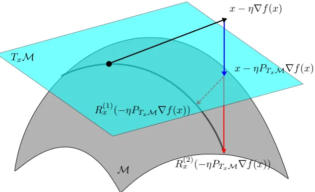
Figure 1: The visualization of gradient descent algorithms on the manifoldM. The black solid line is the Euclidean gradient. The blue solid line is the projection of the Euclidean gradient to the tangent space. The red solid line represents the ortho-graphic retraction, while the red dashed line represents the projective retraction.
Step 2. Calculate its Riemannian gradient, which is the direction of steepest ascent off(x) among all directions in thetangent spaceTxM. This direction is given byPTxM∇f(x),
wherePTxM is the projection operator to the tangent space TxM.
Step 3. Define a retraction Rx that maps the tangent space back to the manifold, i.e.
Rx : TxM → M, where Rx needs to satisfy the conditions in (Vandereycken, 2013,
Definition 2.2). In particular, Rx(0) =x,Rx(y) =x+y+O(kyk2) as y→0, andRx
needs to be smooth. Then the update of the gradient descent algorithmx+ is defined by
x+=Rx(−ηPTxM∇f(x)), (6)
whereη is the step size.
3.2. The geometry of the manifold of low-rank matrices
To apply the gradient descent algorithm in Section 3.1 to the manifold of the low-rank matrices, the projectionPTxM and the retractionRx need to be defined. In this section, we
let Mbe the manifold of allRn1×n2 matrices with rankr and X∈ Mbe a matrix of rank
r and will find the explicit expressions of PTxM and Rx.
The tangent spaceTXMand the retractionRX of the manifold of the low-rank matrices
have been well-studied Absil and Oseledets (2015): Assume that the SVD decomposition of X is X =UΣVT, then the tangent space TXM can be defined by TXM={AVVT + UUTB : for A ∈ Rn1×n1,B ∈ Rn2×n2} according to Absil and Oseledets (2015). The
explicit formula for the projection PTXM is given in (Absil and Oseledets, 2015, (9)):
PTXM(D) =UUTD+DVVT −UUTDVVT, D∈Rn1×n2. (7)
For completeness, a proof of (7) is presented in Appendix.
There are various ways of defining retractions for the manifold of low-rank matrices, and we refer the reader to Absil and Oseledets (2015) for more details. In this work, we consider two types of retractions. One is called theprojective retraction Shalit et al. (2012); Vandereycken (2013), Given anyδ∈TXM, the retraction is defined as the nearest low-rank
matrix toX+δ in terms of Frobenius norm:
R(1)X (δ) = arg min
Z∈M
kX+δ−ZkF. (8)
The solution is the rank-r approximation ofX+δ (for any matrix W, its rank-r approxi-mation is given byPr
i=1σiuiviT, whereσi,ui,vi are the ordered singular values and vectors
of W).
In order to further improve computation efficiency, we also consider the orthographic retraction Absil and Oseledets (2015). Denoted by RX(2)(δ), it is the nearest rank-r matrix toX+δ that their difference is orthogonal to the tangent spaceTXM:
R(2)X (δ) = arg min
Z∈M
kX+δ−ZkF, s.t. hR(2)X (δ)−(X+δ),ZiF = 0 for all Z∈TXM, (9)
and its explicit solution of (9) is given in (Absil and Oseledets, 2015, Section 3.2),
R(2)X (δ) = (X+δ)V[UT(X+δ)V]−1UT(X+δ), (10) and a proof is given in Appendix.
3.3. Derivation of the proposed algorithms
3.3.1. Derivation of Algorithm 1
The gradient descent algorithm (6) for solving (2) can be written as
L(k+1)=RL(k)(−ηPT
L(k)∇f(L
(k))), (11)
where PT
L(k) is defined in (7) and RL(k) is defined in (8) or (10). To derive the explicit
If the absolute values of all entries of Aare different, then we have
∇f(L) =F(L−Y). (12)
The proof of (12) is deferred to Appendix. When some entries of A are equivalent and there is a tie in generating F(L−Y), the objective function could be non-differentiable. However, it can be shown that by arbitrarily breaking the tie, F(L−Y) is a subgradient of f(L).
The corresponding gradient descent method (or subgradient method when f is not differentiable) with projective retraction can be written as follows:
L(k+1) := rank-r approximation of hL(k)−ηPT
L(k)F(L
(k)−Y)i, (13) where the rank-r approximation has been defined after (8). This leads to Algorithm 1 with Option 1.
For the orthographic retraction, i.e., RL(k) defined according to (10), by writing D = F(L(k)−Y), the update formula (11) can be simplified to
L(k+1) := (L(k)−ηD)V(k)[U(k)T(L(k)−ηD)V(k)]−1U(k)T(L(k)−ηD), (14) where U(k) ∈ Rn1×r is any matrix such that its column space is the same as the column
space of L(k); and V(k) ∈ Rn2×r is any matrix such that its column space is the same as
the row space ofL(k). The derivation of (14) is deferred to Appendix, and it can be shown that the implementation of (14) leads to Algorithm 1 with Option 2.
3.3.2. Derivation of Algorithm 2
By a similar argument as in the previous section, we can conclude that when all entries of |L−Y| are different from each other, then applying the same procedure of deriving (12), we have
∇f˜(L) = ˜F(L−Y);
and ˜F(L−Y) is a subgradient when ˜f(L) is not differentiable. Based on this observation, the algorithm under the partially observed setting is identical to (13) or (14), with F replaced by ˜F. This gives the implementation of Algorithm 2.
3.3.3. Basic convergence properties of Algorithms 1 and 2
An interesting topic is that, can we still expect the algorithm to have reasonable basic prop-erties, such as convergence to a critical point? Unfortunately, it is impossible to have such a theoretical guarantee if a fixed step sizeη is chosen: in general, the subgradient method with fixed step size does not have the convergence guarantee if the objective function is non-differentiable. However, if we choose step size with line search, then any accumulation point ofL(k),
b
L, would have the property that either the objective function is not differen-tiable at Lb, or it is a critical point in the sense that its Riemannian gradient is zero. For
example, the line search strategy for Algorithm 1 can be described as follows: start the step sizeηk with a relatively large value, and repeatedly shrinks it by a factor ofβ∈(0,1) such
that the following condition is satisfied: forL(k+1)=RL(k)(−ηkPT
L(k)∇f(L
(k))),
f(L(k))−f(L(k+1))> cηkkPTL(k)∇f(L
where c ∈ (0,1) is prespecified. The argument for convergence follows from the same argument as the proof of (Absil et al., 2009, Theorem 4.3.1).
3.4. Prior works on manifold optimization
The idea of optimization on manifolds has been well investigated in the literature Vander-eycken (2013); Shalit et al. (2012); Absil et al. (2009). For example, Absil et al. Absil et al. (2009) give a summary of many advances in the field of optimization on manifolds. Manifold optimization has been applied to many matrix estimation problems, including re-covering a low rank matrix from its partial entries, i.e., matrix completion Keshavan et al. (2010); Vandereycken (2013); Wei et al. (2016) and robust matrix completion in Cambier and Absil (2016). In fact, the problem studied in this work can be reformulated to the problem analyzed in Cambier and Absil (2016). In comparison, our work studies a different algorithm and gives additional theoretical guarantees.
In another aspect, while Wei et al. (2016) studies matrix completion, it shares some similarities with this work: both works study manifold optimization algorithms and have theoretical guarantees showing that the proposed algorithms can recover the underlying low-rank matrix exactly. In fact, Wei et al. (2016) can be considered as our problem under the partially observed setting, without corruption S∗. It proposes to solve
arg min
L∈Rn1×n2,rank(L)=r
X
(i,j)∈Φ
(Yij −Lij)2,
which can be considered as ˜f in (5) whenγ = 0.
4. Theoretical Analysis
In this section, we analyze the theoretical properties of Algorithms 1 and 2 and compare them with previous algorithms. Since the goal is to recover the low-rank matrix L∗ and the sparse matrix S∗ from Y =L∗+S∗, to avoid identifiability issues, we need to assume thatL∗ can not be both low-rank and sparse. Specifically, we make the following standard assumptions on L∗ andS∗:
Assumption 1 Each row ofS∗ contains at most γ∗n2 nonzero entries and each column of S∗ contains at most γ∗n1 nonzero entries. In other words, for γ∗∈[0,1), assume S∗∈ Sγ∗
where
Sγ∗:=A∈Rn1×n2 | kAi,·k0≤γ∗n2, for 1≤i≤n1;kA·,jk0≤γ∗n1, for 1≤j ≤n2 .
(15)
Assumption 2 The low-rank matrixL∗is not near-sparse. To achieve this, we require that L∗ must be µ-coherent. Given the singular value decomposition (SVD) L∗ = U∗Σ∗V∗T, where U∗ ∈ Rn1×r and V∗ ∈
Rn2×r, we assume there exists an incoherence parameter µ
such that
kU∗k2,∞≤ r
µr n1
, kV∗k2,∞≤ r
µr n2
, (16)
4.1. Analysis of Algorithm 1
With Assumption 1 and 2, we have the following theoretical results regarding the conver-gence rate, initialization, and stability of Algorithm 1:
Theorem 1 (Linear convergence rate, fully observed case) Suppose thatkL(0)−L∗kF ≤
aσr(L∗), where σr(L∗) is the r-th largest singular value of L∗, a ≤ 1/2, γ > 2γ∗ and C1 =
q
4(γ+ 2γ∗)µr+ 4γ−γ∗γ∗ +a2 < 12, then there exists η0 =η0(C1, a) >0 that does not depend on k, such that for all η≤η0,
kL(k)−L∗kF ≤1−1−2C1
8 η
k
kL(0)−L∗kF.
Remark 2 (Choices of parameters). It is shown in the proof that η0 can be set to the solution of the equation
η0(1 +C1)2
1 2+
a2
1−η0(1 +C1)a
= 1
8(1−2C1).
Since the LHS is an increasing function of η0 and is zero when η0 = 0, and its RHS is a positive number.
While C1 < 1/2 requires
p
4γ∗/(γ−γ∗) < 1/2, i.e., γ > 17γ∗. In practice a much
smallerγ can be used. In Section 5, γ = 1.5γ∗ is used and works well for a large number of examples. It suggests that some constants in Theorem 1 might be due to the technicalities in the proof and can be potentially improved.
Remark 3 (Simplified choices of parameters) There exists c1 and c2 such that if a < c1,
γ∗µr < c2 and γ = 65γ∗, then one can choose η0 = 1/8. In this sense, if the initialization of the algorithm is good, then the algorithm can handle γ∗ as large asO(1/µr). In addition, it requires O(log(1/)) iterations to achieve kL(k)−L∗kF/kL(0)−L∗kF < .
Since the statements require proper initializations (i.e., small a), the question arises as to how to choose proper initializations. The work by Yi et al. (2016) shows that if the rank-r
approximation to F(Y) is used as the initialization L(0), then such initialization has the upper boundkL(0)−L∗kaccording to the proofs of (Yi et al., 2016, Theorems 1 and 3) (we borrow this estimation along with the fact thatkL(0)−L∗kF ≤√2rkL(0)−L∗k).
Theorem 4 (Initialization, fully observed case) Ifγ > γ∗ and we initializeL(0) using the rank-r approximation toF(Y), then
kL(0)−L∗kF ≤8γµr
√
2rσ1(L∗).
The combination of Theorem 1, 4 and the fact that γ = O(γ∗) implies that under the fully observed setting, the tolerance of the proposed algorithms to corruption is at most
γ∗ = O(µr√1
rκ), where κ = σ1(L
∗)/σr(L∗) is the condition number of L∗. We also study
Theorem 5 (Stability, fully observed case) Let L be the current value, and let L+ be the next update by applying Algorithm 1 to L for one iteration. Assuming Y=L∗+S∗+ N∗, where N∗ is a random Gaussian noise i.i.d. sampled from N(0, σ2), γ > 10γ∗ and (γ+ 2γ∗)µr <1/64, then there exist C, a, c, η0>0 such that whenη < η0,
P kL+−L∗kF ≤(1−cη)kL−L∗kF for all L∈Γ
→1, as n1, n2→ ∞, (17) where
Γ ={L∈Rn1×n2 : rank(L) =r, Cσp(n
1+n2)rln(n1n2)≤ kL−L∗kF ≤aσr(L∗)k,
Since 1−cη <1, and Theorem 5 shows that when the observationY is contaminated with a random Gaussian noise, if L(0) is properly initialized such that kL(0)−L∗kF < aσr(L∗),
Algorithms 1 will converge to a neighborhood of L∗ given by {L:kL−L∗kF ≤Cσ
p
(n1+n2)rln(n1n2)}
in [−log(kL(0)−L∗kF) + log(Cσp(n1+n2)rln(n1n2))]/log(1−cη) iterations, with prob-ability goes to 1 as n1, n2→ ∞.
4.2. Analysis of Algorithm 2
For the partially observed setting, we assume that each entry of Y =L∗+S∗ is observed with probability p. That is, for any 1≤i≤n1 and 1≤j ≤n2, Pr((i, j)∈Φ) =p. Then we have the following statement on convergence:
Theorem 6 (Linear convergence rate, partially observed case) There exists c > 0 such that for n = max(n1, n2), if p ≥ max(cµrlog(n)/2min(n1, n2),563 γmin(lognn1,n2)), then with probability1−2n−3−6n−1,
kL(k)−L∗kF kL(0)−L∗k
F
≤h
s
1−p2(1−)2
2η
1−C˜1−
ap(1 +)
2(1−a)(1 + ˜C1)
−η2(1 + ˜C 1)2
+η
2a2(p+p)2(1 + ˜C 1)2 1−ηa(p+p)(1 + ˜C1)
ik
(18)
for
˜
C1 = 1
p(1−)
h
6(γ+ 2γ∗)pµr+ 4 3γ
∗
γ−3γ∗( p
p(1 +) +a 2)
2+a2i.
Remark 7 (Choice of parameters) Note that when η is small, the RHS of (18) is in the order of
1−p2(1−)2
1−C˜1−
ap(1 +)
2(1−a)(1 + ˜C1)
η+O(η2).
As a result, to make sure that the RHS of (18)to be smaller than1 for small η, we assume that
1−C˜1−
ap(1 +)
2(1−a)(1 + ˜C1)>0. (19) For example, whenap(1 +) = 4(1−a), it requires thatC˜1<1/3. If (19)holds, then there exists η0 =η0( ˜C1, p, , a) such that for all η≤η0, the RHS of (18) is smaller than1.
Remark 8 (Simplified choice of parameters) There exists {ci}4i=1 >0 such that when < 1/2,a < c1p, γ∗µr < c2 and γ =c3γ∗, then when η <1/8,
kL(k)−L∗k F
kL(0)−L∗k F
≤(1−c4ηp2)k.
Compared with the result in Theorem 1, the addition parameterpappears in both the initial-ization requirement a < c1p as well as the convergence rate. This makes the result weaker, but we suspect that the dependence on the subsampling ratio p could be improved through a better estimation in (39) and the estimation of C˜1 in Lemma 16, and we leave it as a possible future direction.
We present a method of obtaining a proper initialization in Theorem 9. Combining it with Theorem 6, Algorithm 2 allows the corruption level γ∗ to be in the order ofO(µr√p
rκ).
Theorem 9 (Initialization, partially observed case) There exists c1, c2, c3 > 0 such that if γ > 2γ∗, and p ≥ c2(µr
2
2 + α1) logn/min(n1, n2), and we initialize L(0) using the rank-r approximation toF(Y), then
kL(0)−L∗kF ≤16γµrσ1(L∗) √
2r+ 2√2c1σ1(L∗)
with probability at least 1−c3n−1, where σ1(L∗) is the largest singular value ofL∗ . 4.3. Comparison with Alternating Gradient Descent
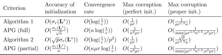
Since our objective functions are equivalent to the objective functions of the alternating gradient descent (AGD) in Yi et al. (2016), it would be interesting to compare these two works. The only difference of these two works lies in the algorithmic implementation: our methods use the gradient descent on the manifold of low-rank matrices, while the methods in Yi et al. (2016) use alternating gradient descent on the factors of the low-rank matrix. In the following we compare the results of both works from four aspects:
1. Accuracy of initialization. What is the largest value t that the algorithm can tolerate, such that for any initializationL(0)satisfyingkL(0)−L∗kF ≤t, the algorithm is guaranteed to converge toL∗?
2. Convergence rate. What is the smallest number of iteration steps k such that the algorithm reaches a given convergence criterion, i.e. kL(k)−L∗kF/kL(0)−L∗kF < ?
3. Corruption level (perfect initialization). Suppose that the initialization is in a sufficiently small neighborhood of L∗ (i.e. there exists a very small 0 >0 such that L(0) satisfies kL(0)−L∗kF < 0), what is the maximum corruption level that can be tolerated in the convergence analysis?
These comparisons are summarized in Table 1. We can see that under the full observed setting, our results remove or reduce the dependence on the condition number κ, while keeping other values unchanged. Under the partially observed setting our results still have the advantage of less dependence onκ, but sometimes require an additional dependence on the subsampling ratio p. The simulation results discussed in the next section also verify that whenκ is large our algorithms have better performance, while that the slowing effect of p under the partially observed setting is not significant. As discussed after Theorem 6, we suspect that this dependence could be removed after a more careful analysis (or more assumptions).
Criterion Accuracy of Convergence Max corruption Max corruption initialization rate (perfect init.) (proper init.)
Algorithm 1 O(σr(L∗)) O(log(1)) O(µr1 ) O(µr11.5κ)
APG (full) O(σr√(L∗)
κ ) O(κlog(
1
)) O(
1
κ2µr) O(
1
max(µr1.5κ1.5,κ2µr))
Algorithm 2 O(√pσr(L∗)) O(log(1)/p2) O(µr1 ) O(
√ p µr1.5κ)
APG (partial) O(σr(L∗)
κ ) O(κµrlog(
1
) O(
1
κ2µr) O(max(µr1.51κ1.5,κ2µr))
Table 1: Comparison of the theoretical guarantees in our work and the alternating gradient descent algorithm in Yi et al. (2016). The four criteria are explained in details in Section 4.3.
Here we use a simple example to give some intuition of why our proposed methods work better than gradient descent method based on factorization. Let us consider the following simple optimization problem:
arg min
z∈Rm
f(z), wherez=Ax+By,
where x,y ∈ Rn and A,B ∈ Rm×n. In this example, (x,y) can be considered as the
“factors” ofz. The gradient descent method on the factors (x,y) is then given by
x+=x−ηATf0(z), y+=y−ηBTf0(z). (20) Writing the update formula (20) in terms ofz, it becomes
z+ =Ax++By+=z−η(AAT +BBT)f0(z).
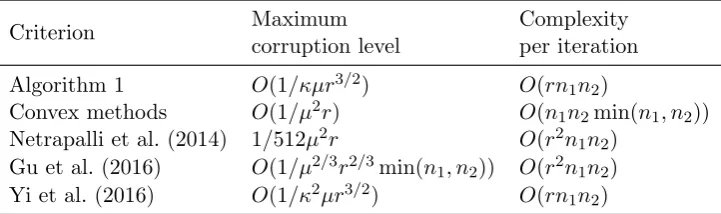
4.4. Comparison with other robust PCA algorithms
In this section we compare our result with other robust PCA methods and summarize them in Table 2. Some criterion in Table 1 are not included since they do not apply. For ex-ample, (Netrapalli et al., 2014, Alternating Projection) only analyzes the algorithm with specific initialization, and the criterion 1 and 3 in Table 1 do not apply to this work. As a result, we only compare the maximum corruption ratio that these methods can han-dle, and the computational complexity per iteration in Table 2. As for the convergence rate, it depends on assumptions on parameters such as the coherence parameter, rank, and the size of the matrix: The alternating projection Netrapalli et al. (2014) requires 10 log(4n1µ2rkY−L(0)k2/
√
n1n2) iterations to achieve an accuracy , under the assump-tions thatγ∗ <1/512µr2and a tuning parameter is chosen to be 4µ2r√n1n2. The alternat-ing minimization method Gu et al. (2016) have the guarantee that ifkL(1)−L∗k2 ≤σ1(L∗), then
kL(k+1)−L∗kF ≤σ1
96√2νµ√r(s∗/d)3/2κσ1 1−24√2νµ√r(s∗/d)3/2κσ
1
!k
kL(1)−L∗kF,
whereν is a parameter concerning the coherence of L∗,s∗ is the number of nonzero entries in S∗, d= min(n1, n2). As a result s∗/d is approximately γ∗max(n1, n2) in our notation. If ν is in the order of O(1), then this results requires that µ√rκσ1max(n1, n2)3/2γ∗3/2 ≤
O(1), which is more restrictive than our assumption in Theorem 1 that γ∗µr ≤ O(1). Convex methods usually have convergence rate guarantees based on convexity, for example, the accelerated proximal gradient method Toh and Yun (2010) has a convergence rate of
O(1/k2). While it is a slower convergence rate compared to the result in Theorem 1 in this work or the results in Netrapalli et al. (2014); Gu et al. (2016) and it does not necessarily converge to the correct solution, this result does not depend on any assumption on the low-rank matrix and the corruption ratio.
Criterion Maximum Complexity
corruption level per iteration
Algorithm 1 O(1/κµr3/2) O(rn1n2)
Convex methods O(1/µ2r) O(n1n2min(n1, n2)) Netrapalli et al. (2014) 1/512µ2r O(r2n1n2)
Gu et al. (2016) O(1/µ2/3r2/3min(n1, n2)) O(r2n1n2) Yi et al. (2016) O(1/κ2µr3/2) O(rn1n2)
Table 2: Comparison of the theoretical guarantees in our work and some other robust PCA algo-rithms.
The stability in Theorem 5 is comparable to analysis in Netrapalli et al. (2014) (the works Gu et al. (2016) and (Yi et al., 2016, Alternating Gradient Descent) do not have stability analysis). The work Netrapalli et al. (2014) assumes that kN∗k∞< σr(L∗)/100n2 and proves that the output of their algorithmLb satisfies
kLb−L∗kF ≤+ 2µ2r
7kN∗k2+
8√√n1n2
r kN
∗k ∞
where is the error of the algorithm when there is no noise. If N∗ is i.i.d. sampled from
N(0, σ2), this result suggests that kLb−L∗kF is bounded above by+O(µ2
√
rn1n2σ). In comparison, Theorem 5 suggests that after a few iterations,kL(k)−L∗kF is bounded above by Cσp(n1+n2)rln(n1n2) with high probability, which is a tighter upper bound.
5. Simulations
In this section, we test the performance of the proposed algorithms by simulated data sets and real data sets. The MATLAB implementation of our algorithm used in this section is available at https://sciences.ucf.edu/math/tengz/. For simulated data sets, we generate L∗ by UΣVT, where U ∈ Rn1×r and V ∈
Rn2×r are random matrices that i.i.d.
sampled from N(0,1), and Σ ∈ Rn1×r is an diagonal matrix. As for S∗ ∈ Rn1×n2, each
entry is sampled from N(0,100) with probability q, and is zero with probability 1−q. That is, q represents the level of sparsity in the sparse matrix S∗. It measures the overall corruption level of Y and is associated with the corruption level γ∗ (γ∗ measures the row and column-wise corruption level). For the partially observed case, we assume that each entry ofY is observed with probabilityp.
5.1. Choice of parameters
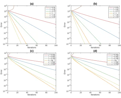
We first investigate the performance of the proposed algorithms, in particular, the depen-dence on the parameters η andγ. In simulations, we let [n1, n2] = [500,600],r = 3,Σ=I, and q= 0.02. For the partially observed case, we letp= 0.2.
The first simulation investigates the following questions:
• Should we use the Algorithms 1 and 2 with Option 1 or Option 2?
• What is the appropriate choice of the step size η?
The simulation results for Option 1 an 2 with various step sizes are visualized in Figure 2, which show that the two options perform similarly. Usually the algorithms converge faster when the step size is larger. However, if the step size is too large then it might diverge. As a result, we use the step sizeη= 0.7 for Algorithm 1 and 0.7/p for Algorithm 2 for the following simulations.
The second simulation concerns the choice of γ. We test γ =cγ∗ for a few choices of c
(γ∗ can be calculated from the zero pattern of S). Figure 5.1 shows that if γ is too small, for example, 0.5γ∗, then the algorithm fail to converge to the correct solution; and if γ is too large, then the convergence is slow. Following these observations, we use γ = 1.5γ∗ as the default choice of the following experiments, which is also used in Yi et al. (2016).
5.2. Performance of the proposed algorithm
In this section, we analyze the convergence behavior as the parameters (overall ratio of corrupted entriesq, condition numberκ, rankr, subsampling ratiop) changes and visualized the result in Figure 4.
0 20 40 60 80 100 Iterations 10-10 10-8 10-6 10-4 10-2 100 102 104 Error (a)
2 = 0.2
2 = 0.4
2 = 0.7
2 = 1
2 = 1.5
2 = 2.5
0 20 40 60 80 100
Iterations 10-10 10-8 10-6 10-4 10-2 100 102 104 Error (b)
2 = 0.2
2 = 0.4
2 = 0.7
2 = 1
2 = 1.5
2 = 2.5
0 20 40 60 80 100
Iterations 10-10 10-8 10-6 10-4 10-2 100 102 104 Error (c)
2 = 0.2/p
2 = 0.4/p
2 = 0.7/p
2 = 1/p
2 = 1.5/p
2 = 2.5/p
0 20 40 60 80 100
Iterations 10-10 10-8 10-6 10-4 10-2 100 102 104 Error (d)
2 = 0.2/p
2 = 0.4/p
2 = 0.7/p
2 = 1/p
2 = 1.5/p
2 = 2.5/p
Figure 2: The dependence of the estimation error on the number of iterations for differ-ent step sizes η (a) Algorithm 1 (Option 1); (b) Algorithm 1 (Option 2); (c) Algorithm 2 (Option 1); (d) Algorithm 2 (Option 2).
0 100 200 300 400 500
Iterations 10-8 10-6 10-4 10-2 100 102 Error (a)
. = 0.5.* . = .* . = 1.5.* . = 2.* . = 3.* . = 4.* . = 6.*
0 100 200 300 400 500
Iterations 10-3 10-2 10-1 100 101 102 103 Error (b)
. = 0.5.* . = .* . = 1.5.* . = 2.* . = 3.* . = 4.* . = 6.*
converges slower with more corruption, which is expected since there is fewer information available. However, the algorithm still converges even with an overall corruption level at 0.4.
Figure 4(b) shows the simulation for rankr, we use the setting in Section 5.1, but replace
r by r= 3,10,30,100,300 respectively. Simulations show that the algorithm works fine for rank r= 3,10,30,100 and it converges slower for rank r= 300.
Figure 4(c) shows the simulation for condition number κ of L, we use the setting in Section 5.1, but replace Σ by Σ = diag(1,1,1/κ) and try various values of κ. While the algorithm converges for κ up to 30 in the simulation, for larger κ the algorithm converges slowly at the beginning, and then decreases quickly to zero. We suspect that the initial-ization is not sufficiently good and it takes a while for the algorithm to reach the “local neighborhood of convergence”. We also remark thatL with a very large condition number, e.g. κ= 100, is generally challenging for any nonconvex optimization algorithm, as shown in Figure 5, Setting 4. It is because that when κ is large, the solution is close to a matrix with rank less than r – a singular point on the manifold of the matrices of rank r, which gives a geometry of manifold that is not “smooth” enough. We observe that whenκ= 100, our algorithm performs well if the rank r is set to 2 (instead of the true value 3)—in fact, when κ = 100, the underlying matrix is approximately of rank 2 since the third singular value is very small.
We test the algorithm with various matrix sizes using the setting in Section 5.1 and set [n1, n2] = [1000,1200],[5000,6000],[10000,12000]. Figure 4(d) shows that Algorithm 1 converges quickly for all of the choices within a few iterations.
In the last simulation, we test Algorithm 2 under the setting in Section 5.1 with various choices of the subsampling ratiop. Figure 4(e) shows suggest that the algorithm converges forp as small as 0.1, though the convergence rate is slow for small p.
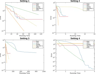
5.3. Comparison with other robust PCA algorithms
In this section, we compare our algorithm with the accelerated proximal gradient method (APG) and the alternating direction method of multiplier (ADMM) based on convex relax-ation (1); the robust matrix completion algorithm (RMC) Cambier and Absil (2016) based on manifold optimization problem
arg min rank(L)=r
X
(i,j)∈Φ
kLij −Yijk+λ
X
(i,j)6∈Φ L2ij,
0 500 1000 1500
Iterations
10-10 10-8 10-6 10-4 10-2 100 102 104
Error
(a)
q = 0.4 q = 0.3 q = 0.2 q = 0.1
0 50 100 150
Iterations
10-10 10-5 100
Error
(b)
rank = 3 rank = 10 rank = 30 rank = 100 rank = 300
0 500 1000 1500 2000 2500 3000
Iterations
10-10 10-5 100
Error
(c)
5 = 1
5 = 3
5 = 10
5 = 30
5 = 100
0 10 20 30 40 50
Iterations
10-10 10-8
10-6 10-4 10-2 100 102 104
Error
(d)
[n1,n2] = [500,600] [n1,n2] = [1000,1200] [n
1,n2] = [5000,6000]
[n
1,n2] = [10000,12000]
0 200 400 600 800 1000
Iterations
10-10 10-5 100
Error
(e)
p = 1 p = 0.5 p = 0.2 p = 0.1 p = 0.05
0 20 40 60 80 100 120
Running Time
10-10 10-5 100
Error
Setting 1
RMC APG ADMM Algorithm 1 AGD
0 5 10 15 20
Running Time
10-15 10-10 10-5 100 105
Error
Setting 2
RMC APG ADMM Algorithm 1 AGD
0 200 400 600 800 1000
Running Time
10-15 10-10 10-5 100 105
Error
Setting 3
RMC APG ADMM Algorithm 1 AGD
0 1 2 3 4
Running Time
10-4 10-3 10-2 10-1 100
101 102 103
Error
Setting 4
RMC APG ADMM Algorithm 1 AGD
Figure 5: The comparison of the performance of the algorithms under the fully observed setting. The running time is measured in seconds.
• Setting 1: same setting as in Section 5.1.
• Setting 2 (large condition number): replace Σ by diag(1,1,0.1) in Setting 1.
• Setting 3 (large matrix): replace n1 and n2 by 3000 and 4000 in Setting 1. • Setting 4 (large condition number): replace Σ by diag(1,1,0.01) in Setting 1.
0 1 2 3 4 5
Running Time
10-8 10-6 10-4 10-2 100 102 104
Error
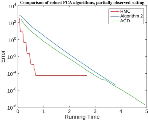
Comparison of robust PCA algorithms, partially observed setting
RMC Algorithm 2 AGD
Figure 6: The comparison of the performances of the algorithms under the partially ob-served setting. The running time is measured in seconds.
practice, we observed that if the initialization is well chosen and close to the true L∗, then Algorithm 1 converges quickly to the correct solution.
We also compare the performance of RMC, AGD and Algorithm 2 under the partially observed setting. We use Setting 1 with p = 0.3 and visualize the result in Figure 6. The results are similar to that of the fully observed setting: AGD and Algorithm 2 are comparable and RMC converges faster at the beginning, but then does not achieve higher accuracy, possibly due to their choice of the regularization parameter.
We also test the proposed algorithms in a real data application for video background subtraction. We adopt the public data setShoppingmallstudied in Yi et al. (2016),1 A few frames are visualized in the first column of Figure 7. There are 1000 frames in this video sequence, represented by a matrix of size 81920×1000, where each column corresponds to a frame of the video and each row corresponds to a pixel of the video. We apply our algorithms with r = 3 and γ∗ = 0.1, p = 0.5 for the partially observed case, the step size
η = 0.7. We stop the algorithm after 100 iterations. Figure 7 shows that our algorithms obtain desirable low-rank approximations within 100 iterations.
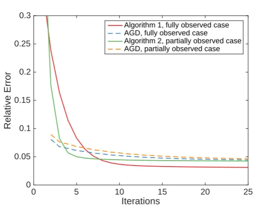
In Figure 8, we compare our algorithms with APG in terms of the convergence of the objective function value. In this figure, the relative error is defined askF(L−Y)kF/kYkF, a scaled objective value. A smaller relative error implies a better low-rank approximation. Figure 8 shows out that our algorithms can obtain smaller objective values within 100 iterations under both fully observed and partially observed cases.
Figure 7: The performance of Algorithms 1 and 2 in video background subtraction, with three rows representing three frames in the video sequence. For Algorithm 2, a subsampling ratio ofp= 0.5 is used.
0 5 10 15 20 25
Iterations
0 0.05 0.1 0.15 0.2 0.25 0.3
Relative Error
Algorithm 1, fully observed case AGD, fully observed case
Algorithm 2, partially observed case AGD, partially observed case
6. Conclusion
This paper proposes two robust PCA algorithms (one for fully observed case and one for partially observed case) based on the gradient descent algorithm on the manifold of low-rank matrices. Theoretically, compared with the gradient descent algorithm with matrix factorization, our approach has a faster convergence rate, better tolerance of the initializa-tion accuracy and corrupinitializa-tion level. The approach removes or reduces the dependence of the algorithms on the condition number of the underlying low-rank matrix. Numerically, the proposed algorithms performance is less sensitive to the choice of step sizes. We also find that under the partially observed setting, the performance of the proposed algorithm is not significantly affected by the presence of the additional dependence on the observation probability. Considering the popularity of the methods based on matrix factorization, it is an interesting future direction to apply manifold optimization to other low-rank matrix estimation problems.
Acknowledgements
Appendix for “Robust PCA by Manifold Optimization"
A. Technical Derivations in Section 3
Verification of (7). Formula (7) can be verified as follows. Let h·iF be the Frobenius
inner product of two matrices, then
hD−PTXM(D),AVVTiF =h(I−UUT)D(I−VVT),AVVTiF
=h(I−UUT)D(I−VVT)VVT,AiF =h0,AiF = 0
and similarly hD − PTXM(D),UUTBiF = 0. As a result, hD − PTXM(D),AVVT +
UUTBiF = 0 for all A ∈Rn1×n1 and B ∈Rn2×n2, which verifies formula (7) by showing
thatD−PTXM(D) is orthogonal to TXM.
Verification of (10). It is clear thatR(2)X (δ) defined in (10) has rankr; and to show that hR(2)X (δ)−(X+δ),ZiF = 0 for allZ∈TXM, we first write this property as [R(2)X (δ)−(X+
δ)] ⊥ TXM for simplicity, and since TXM = {AVVT +UUTB : for A ∈ Rn1×n1,B ∈ Rn2×n2}, we just need to show that hR(2)X (δ)−(X+δ),AVVT +UUTBiF = 0 for all
A∈Rn1×n1 andB∈Rn2×n2. This is easy to verify, because we haveR(2)X (δ)V= (X+δ)V,
hR(2)X (δ)−(X+δ),AVVTiF =h(RX(2)(δ)V−(X+δ)V)VT,AiF =h0,AiF = 0, (21)
Similarly, we can easily verify that UTR(2)X (δ) = UT(X +δ), we have hR(2)X (δ) −(X+
δ),UUTBiF = 0, and therefore [R(2)X (δ)−(X+δ)] ⊥ TXM. As a result, there exists a
uniqueR(2)X such that rank(R(2)X ) =r and [RX(2)(δ)−(X+δ)]⊥TXM.
Verification of (12). We first define the operatorS :Rn1×n2 →Rn1×n2 such thatF(A) =
S(A)◦A (◦ represents the elementwise product), i.e.,
S(A) =
(
0, if|Aij|>|Ai,·|[γ] and|Aij|>|A·,j|[γ],
1, otherwise.
Then if the absolute values of all entries of A are different, the sparsity pattern does not change under a small perturbation, i.e.,S(A) =S(A+∆).Then by definition off(·),
f(L+∆)−f(L) = 1
2kS(L−Y+∆)◦(L−Y+∆)k 2
F −
1
2kS(L−Y)◦(L−Y)k 2
F
=1
2kS(L−Y)◦(L−Y+∆)k 2
F −
1
2kS(L−Y)◦(L−Y)k 2
F
=hS(L−Y)◦(L−Y),∆iF +O(k∆k2
F),
where◦represents the Hadamard product, i.e., the elementwise product between matrices.
Verification of (14). It is sufficient to prove the case whereU(k) and V(k) are given by the SVD decomposition L(k)=U(k)Σ(k)V(k)T. Denote D=∇f(L(k)) =F(L(k)−Y). Set X=L(k) and δ =−ηPT
L(k)M(D) in (10), we have
L(k+1) := (L(k)−ηPT
L(k)M(D))V
(k)[U(k)T(L(k)−ηPT
L(k)M(D))V
(k)]−1 (22) U(k)T(L(k)−ηPT
On the other hand, from (7) we have the projection
PT
L(k)M(D) =U
(k)U(k)TD+DV(k)V(k)T −U(k)U(k)TDV(k)V(k)T.
As a result
PTL(k)M(D)V
(k)= [U(k)U(k)TD+DV(k)V(k)T −U(k)U(k)TDV(k)V(k)T]V(k)
=U(k)U(k)TDV(k)+DV(k)V(k)TV(k)−U(k)U(k)TDV(k)V(k)TV(k)=DV(k) (23) and similarly,
U(k)TPT
L(k)M(D) =U
(k)TD. (24)
Combining (23), (24) with (22), the update formula (14) is verified.
B. Proof of Theorem 1
In this proof, we will investigatekL+−L∗kF, where
L+=RL(−ηPTLF(L−Y)).
It is sufficient to prove that when kL−L∗k ≤ aσr(L∗) with the value a satisfying the conditions in Theorem 1, then
kL+−L∗kF ≤
1−1−2C1
8 η
kL−L∗kF. (25)
To prove (25), we first introduce three auxiliary lemmas.
Lemma 10 (a) Let D=L−L∗−F(L−Y) =L−L∗−F(L−L∗−S∗), then
kDk2F ≤C12kL−L∗k2F. (26) (b) For the noisy setting where Y =L∗+S∗ +N∗, and D0 = L−L∗−N∗−F(L−Y),
we have
kD0k2F ≤2C12kL−L∗k2F + 2(γ+ 5γ∗)N1, (27) where N1 =n2Pni=11 |N∗i,·|max+n1Pnj=12 |N∗·,j|max.
Lemma 11 If kL−L∗kF ≤aσr(L∗) and a≤1, then
k(L−L∗)−PTL(L−L∗)kF ≤ a
2(1−a)kL−L
∗k
F, (28)
k(L−L∗)−PTL∗(L−L∗)kF ≤ a
2kL−L
∗k
F. (29)
Lemma 12 ForX∈TLM, then
kR(Li)(X)−(L+X)kF ≤
kXk2
F
2(σr(L)− kXk)
To prove (25), first we note that
kL−L∗k2F − kL−ηPTLF(L−Y)−L∗k2F
=kL−L∗k2F − kL−L∗k2F + 2ηhL−L∗, PTLF(L−Y)iF − kηPTLF(L−Y)k2F
=2ηhL−L∗, PTLF(L−Y)iF − kηPTLF(L−Y)k2F
=2ηhL−L∗, PTL(L−L∗)−PTL(L−L∗−F(L−Y))iF −η2kPTLF(L−Y)k2F
=2ηhPTL(L−L∗), PTL(L−L∗)−PTLDiF −η2kPTLF(L−Y)k2F
≥2η(kPTL(L−L∗)kF2 − kDkFkPTL(L−L∗)kF)−η2(kL−L∗kF +kDkF)2. (30)
The fourth line is obtained by PTL(L−L∗ −F(L −Y)) = L −L∗ −PTLF(L −Y)iF.
The fifth line is because L−L∗ =PTL(L−L∗) +PTL⊥(L−L∗). The last line uses Cauchy-Schwarz inequalityhPTL(L−L∗), PTLDiF ≤ kDkFkPTL(L−L∗)kF and triangular inequality
kPTLF(L−Y)kF ≤ kL−L∗kF +kPTL(D)kF ≤ kL−L∗kF +kDkF. Lemma 11 and the
assumptionskL−L∗kF ≤aσr(L∗) and
q
1−(2(1a−a))2> 1 2 imply kPTL(L−L∗)kF ≥
1
2kL−L
∗k
F. (31)
Combining it with the estimation of kDkF in Lemma 10, we have kL−L∗k2F − kL−ηPTLF(L−Y)−L∗k2F
≥η(1
2 −C1)kL−L
∗k2
F −η2(1 +C1)2kL−L∗k2F. (32)
When ths RHS of (32) is positive (i.e., when (1−2C1)≥2η(1 +C1)2), (32) implies kL− L∗kF >kL−ηPTLF(L−Y)−L∗kF and
kL−L∗kF − kL−ηPTLF(L−Y)−L∗kF
≥η( 1
2 −C1)kL−L
∗k2
F −η2(1 +C1)2kL−L∗k2F
kL−L∗kF +kL−ηPTLF(L−Y)−L ∗k
F
≥1 2
η(1
2 −C1)−η
2(1 +C 1)2
kL−L∗kF. (33)
In addition,
kPTLF(L−Y)kF ≤ kF(L−Y)kF =kL−L∗kF +kDkF ≤(1 +C1)kL−L∗kF (34)
and Lemma 12 give
kL+−L∗kF − kL−ηPTLF(L−Y)−L ∗k
F ≤ kL−ηPTLF(L−Y)−L
+k
F
≤ η
2kPTLF(L−Y)k2
F σr(L∗)−ηkPTLF(L−Y)kF
≤ η
2a2(1 +C 1)2 1−ηa(1 +C1)
kL−L∗kF. (35)
Combining (33) and (35),
kL−L∗kF − kL+−L∗kF kL−L∗kF
≥ 1
4η(1−2C1)−η
2(1 +C 1)2
1 2 +
a2
1−η(1 +C1)a
.
Therefore, Theorem 1 is proved when C1<1/2, andη0 is chosen such that
η0(1 +C1)2
1 2+
a2
1−η0(1 +C1)a
≤ 1
C. Proof of Theorem 5
The proof of the noisy case also follows similarly from the proofs of Theorem 1 and 6. Note that
F(L−Y) =L−L∗−N∗−D0,
and defineQ=PTL(L−L∗), then following the proof of Theorem 1 and applying Lemma 10
(b), we have
kL−L∗k2F − kL−ηPTLF(L−Y)−L∗k2F
=2ηhL−L∗, PTLF(L−Y)iF +O(η2) = 2ηhPTL(L−L∗), PTLF(L−Y)iF +O(η2)
=2ηhPTL(L−L∗), PTL(L−L∗−N∗−D0)iF +O(η2)
≥2η
kQk2F − hN∗,QiF − kQkF
q
2C12kL−L∗k2
F + 2(γ+ 5γ∗)N1
+O(η2).
In addition, (35) gives
kL+−LkF − kL−ηPTLF(L−Y)−L ∗k
F
=O(η2).
Combining it with the estimation of C1,N1, and hN∗,QiF in Lemma 13 and the fact that
(1− a
2(1−a))kL−L
∗k
F ≤ kQkF ≤(1 + 2(1a−a))kL−L∗kF (which follows from Lemma 11),
the Theorem is proved.
Lemma 13 If N∗∈Rn1×n2 is elementwisely i.i.d. sampled from N(0, σ2), then
(a) with probability 1−n74 1n72
, Pn1
i=1(|N∗i,·|max)2 ≤16σ2n1ln(n1n2), and Pnj=12 (|N∗·,j|max)2≤
16σ2n2ln(n1n2), and as a result, N1≤32σ2n1n2ln(n1n2).
(b) There exists C6 >0 such that as n1+n2→ ∞, the probability that hN∗, PTL(L−L∗)iF ≤
1
4kPTL(L−L
∗)k2
F (36)
holds for all{L:C6σ
p
(n1+n2)rln(n1n2)≤ kL−L∗kF ≤aσr(L∗)} converges to 1.
D. Proof of Theorem 6
This proof borrows two lemmas from (Yi et al., 2016, Lemmas 9, 10) as follows.
Lemma 14 (Yi et al., 2016, Lemma 9) There exists c > 0 such that for all 0 < < 1, if p ≥ cµrlog(n)/2min(n1, n2), then with probability at least 1−2n−3, for all X in the tangent plane TL∗, i.e., all X that can be written as L∗A+BL∗, where A ∈ Rn2×n2 and
B∈Rn1×n1,
(1−)kXk2F ≤ 1
pkPΦXk
2
F ≤(1 +)kXk2F.
Lemma 15 (Yi et al., 2016, Lemma 10) If p≥ 56 3
logn
γmin(n1,n2), the with probability at least
1−6n−1, the number of entries in Φ per row is in the interval [pn2/2,3pn2/2], and the number of entries in Φper column is in [pn1/2,3pn1/2].
Lemma 16 When the events in Lemmas 14 and 15 hold, forD˜ =PΦ[L−L∗−F˜(L−Y)] we have
kD˜k2F ≤C˜12kL−L∗k2F, (37) with
˜
C1 = 1
p(1−)
h
6(γ+ 2γ∗)pµr+ 4 3γ
∗
γ−3γ∗( p
p(1 +) +a 2)
2+a2i.
The proof of Theorem 6 is parallel to the proof of Theorem 1, with L+ defined slightly differently by
L+=RL(−ηPTLF˜(L−Y)).
DefiningPΦ:Rn1×n2 →Rn1×n2 by
[PΦX]ij =
(
Xij, if (i, j)∈Φ, 0, if (i, j)∈/ Φ.
Then ˜F(L−Y) =PΦF˜(L−Y). Following a similar analysis as (30),
kL−L∗k2F − kL−ηPTLPΦF˜(L−Y)−L∗k2F
=2ηhL−L∗, PTLPΦF˜(L−Y)iF − kηPTLPΦF˜(L−Y)k2F
≥2ηhPΦPTL(L−L∗), PΦF˜(L−Y)iF − kηPΦF˜(L−Y)k2F
≥2ηhPΦ(L−L∗)−PΦPTL⊥(L−L∗), PΦ(L−L∗)−D˜iF −η2(kPΦ(L−L∗)kF +kD˜kF)2,
(38)
here PTL⊥ represents the projector to the subspace orthogonal to TL. Lemma 11 and
Lemma 14 imply
kPΦPT⊥L(L−L ∗)k
F
kPΦ(L−L∗)kF
≤ kP
⊥
TL(L−L ∗)k
F
kPΦ(L−L∗)kF
≤ ap(1 +)
2(1−a), (39)
and combining it with the estimation of ˜D in Lemma 16, the RHS of (38) is larger than
kPΦ(L−L∗)k2F
2η
1−C˜1−
ap(1 +)
2(1−a)(1 + ˜C1)
−η2(1 + ˜C1)2
. (40)
In addition, Lemma 14 implies
kPΦF˜(L−Y)kF ≤ kPΦ(L−L∗)kF +kPΦD˜kF
≤(1 + ˜C1)kPΦ(L−L∗)kF,
≤(1 + ˜C1)p(1 +)kL−L∗k and combining it with Lemma 12,
kL+−L∗kF − kL−ηPTLPΦF˜(L−Y)−L ∗k
F ≤
η2a2(p+p)2(1 + ˜C1)2 1−ηa(p+p)(1 + ˜C1)
Combining it with (40) and Lemma 11, we have
kL+−L∗kF kL−L∗kF
≤
s
1−p2(1−)2
2η
1−C˜1−
ap(1 +)
2(1−a) (1 + ˜C1)
−η2(1 + ˜C 1)2
+η
2a2(p+p)2(1 + ˜C 1)2 1−ηa(p+p)(1 + ˜C1)
,
and Theorem 6 is proved.
E. Proof of Lemmas
Lemma 10(a) Proof By the definition of F, for any matrix A, A−F(A) is a sparse matrix, therefore
D=L−L∗−S∗−F(L−L∗−S∗) +S∗
is a sparse matrix. Denote the locations of the nonzero entries ofD byS, and divide it into two sets S1∪ S2 defined as follows:
S1 ={(i, j) :|[L−L∗−S∗]ij|>|[L−L∗−S∗]i,·|[γ]and|[L−L∗−S∗]ij|>|[L−L∗−S∗]·,j|[γ]},
and
S2={(i, j)∈ S/ 1 :Dij = [L−L∗]ij−F(L−L∗−S∗)ij 6= 0}.
For (i, j) ∈ S1, [F(L−L∗−S∗)]ij = 0. As a result, Dij = [L−L∗]ij. In addition, by
definition ofF(·), each row or column of Dhas at most γ percentage of points inS1. For (i, j)∈ S2, since [F(L−L∗−S∗)]ij = [L−L∗−S∗]ij, we have Dij =S∗ij 6= 0. By
Assumption 1, therefore, for each row or column of D, at most γ∗ percentage of points lie inS2.
Combine the results
|[L−L∗−S∗]i,·|[γ]≤ {|[L−L∗]i,·|+|[S∗]i,·|}[γ]≤ |[L−L∗]i,·|[γ−γ ∗]
,
|[L−L∗−S∗]j,·|[γ]≤ {|[L−L∗]j,·|+|[S∗]j,·|}[γ]≤ |[L−L∗]j,·|[γ−γ ∗]
,
with [F(L−L∗−S∗)]ij = [L−L∗−S∗]ij, we have for (i, j)∈ S2 |Dij|=|[L−L∗−F(L−L∗−S∗)]ij|
≤|[L−L∗]ij|+|F(L−L∗−S∗)]ij|
≤|[L−L∗]ij|+ max(|[L−L∗−S∗]i,·|[γ],|[L−L∗−S∗]·,j|[γ])
≤|[L−L∗]ij|+ max(|[L−L∗]i,·|[γ−γ ∗]
,|[L−L∗]·,j|[γ−γ
∗]
).
kDk2F = X (i,j)∈S
D2ij = X (i,j)∈S1
D2ij+ X (i,j)∈S2
D2ij ≤ X (i,j)∈S1
[L−L∗]2ij
+ X
(i,j)∈S2 n
|[L−L∗]ij|+ max(|[L−L∗]i,·|[γ−γ ∗]
,|[L−L∗]·,j|[γ−γ
∗]
)o2
≤ X
(i,j)∈S1
[L−L∗]2ij + 2 X (i,j)∈S2
[L−L∗]2ij+ 2 X (i,j)∈S2
max{|[L−L∗]i,·|[γ−γ ∗]
,|[L−L∗]·,j|[γ−γ
∗]
}2
≤ X
(i,j)∈S1
[L−L∗]2ij + 2 X (i,j)∈S2
[L−L∗]2ij+ 2 X (i,j)∈S2
{|[L−L∗]i,·|[γ−γ ∗]
+|[L−L∗]·,j|[γ−γ
∗]
}2
≤ X
(i,j)∈S1
[L−L∗]2ij + 2 X (i,j)∈S2
[L−L∗]2ij+ 4 X (i,j)∈S2
{|[L−L∗]i,·|[γ−γ ∗]
}2+{|[L−L∗]·,j|[γ−γ
∗]
}2
≤ X
(i,j)∈S
[L−L∗]2ij+ X (i,j)∈S2
[L−L∗]2ij + 4 γ
∗
γ−γ∗kL−L ∗k2
F
≤2 X (i,j)∈S
[PTL∗(L−L ∗)]2
ij + 2
X
(i,j)∈S2
[PTL∗(L−L ∗)]2
ij + 4
γ∗
γ−γ∗kL−L ∗k2
F
+ 2 X
(i,j)∈S
[L−L∗−PTL∗(L−L ∗)]2
ij + 2
X
(i,j)∈S2
[L−L∗−PTL∗(L−L ∗)]2
ij
≤2 X
(i,j)∈S
[PTL∗(L−L ∗
)]2ij + 2 X (i,j)∈S2
[PTL∗(L−L ∗
)]2ij + 4 γ
∗
γ−γ∗kL−L ∗k2
F
+ 4kL−L∗−PTL∗(L−L ∗)k2
F. (41)
Note that from line 5 to line 6, we used the fact that for x∈Rn, and k≤n
k(x(k))2 ≤(x(k))2+ (x(k+1))2+· · ·+ (x(n−1)) + (x(n))≤(x(1)) +· · ·+ (x(n)) =kxk2F,
wherex(k) is the k-th order statistics of x1, . . . , xn, i.e. the k-th smallest value. This gives us
(γ−γ∗)n2|[L−L∗]i,·|[γ−γ ∗]
≤ k[L−L∗]i,·k22; (γ−γ∗)n2|[L−L∗]·,j|[γ−γ
∗]
≤ k[L−L∗]·,jk22. Therefore
X
(i,j)∈S2
|[L−L∗]i,·|[γ−γ ∗]
≤ γ
∗n
2 (γ−γ∗)n
2
k[L−L∗]i,·k2F; (42)
X
(i,j)∈S2
|[L−L∗]·,j|[γ−γ
∗]
≤ γ
∗n
1 (γ−γ∗)n1
k[L−L∗]·,jk2F. (43)
The valuesγ∗n2 and γ∗n1 in the numerator of the right hand sides in 42 and 43 are due to the fact that, in each row or column of D, at mostγ∗ percentage of points lie in S2.
On the other hand, Lemma 11 implies
kL−L∗−PTL∗(L−L∗)kF ≤ a
2kL−L
∗k
In addition, using the fact that there exists A ∈ Rn1×r and B ∈
Rn2×r, such that
PTL∗(L−L
∗) =AVT +UBT and kP
TL∗(L−L ∗)k2
F =kAVTk2F +kUBTk2F, and that for
each row or column, at mostγ+γ∗ percentage of points lie in S, we have
X
(i,j)∈S
[PTL∗(L−L ∗
)]2ij ≤2 X (i,j)∈S
[k(AVT)ijk2+k(UBT)ijk2]
≤2(γ+γ∗)µr X
1≤i≤n1,1≤j≤n2
[k(AVT)ijk2+k(UBT)ijk2] = 2(γ+γ∗)µrkPTL∗(L−L∗)k2F
≤2(γ+γ∗)µrkL−L∗k2
F. (45)
Similarly, kAk2,∞= maxkzk2=1kAzk∞ X
(i,j)∈S2
[PTL∗(L−L∗)]2ij ≤2γ∗µrkL−L∗k2F, (46)
Combining (41)-(46), (26) is proved.
Lemma 10(b) Proof Let L0 =L−N∗, then applying the fact that for any x,y∈Rn,
|[x+y]|[γ]≤ |[x]|[γ]+|[x]|max,
where|[x]|max represents the largest value of|[x]|. We have kD0k2F ≤ X
(i,j)∈S
[L0−L∗]2ij + X (i,j)∈S2
[L0−L∗]2ij
+ 2 X
(i,j)∈S2
{(|[L0−L∗]i,·|[γ−γ ∗]
)2+ (|[L0−L∗]·,j|[γ−γ
∗]
)2}
≤2
X
(i,j)∈S
[L−L∗]2ij +|N∗ij|2+ X (i,j)∈S2
[L−L∗]2ij+|N∗ij|2
+ 4 X
(i,j)∈S2
{(|[L0−L∗]i,·|[γ−γ ∗]
)2+ (|N∗i,·|max)2+ (|[L0−L∗]·,j|[γ−γ
∗]
)2+ (|N∗·,j|max)2}
≤2C12kL−L∗k2
F + 2(γ+ 5γ∗)N1,
where the last inequality follows from the proof of part (a) and the definition of N1.
Lemma 11 Proof Let the SVD decomposition of L∗ be L∗ = UΣV, U⊥ and V⊥ be orthogonal matrices of sizes Rn1×(n1−r) and Rn2×(n2−r) such that Col(U⊥) ⊥ Col(U) and
Col(V⊥) ⊥ Col(V) (here Col(U) represents the subspace spanned by the columns of U). Let
L∗(1,1) ≡UTL∗V, L∗(1,2)≡UTL∗V⊥,
Since rank(L∗) =r, we have
L∗(2,2) =L∗(2,1)L∗(1,1)−1L∗(1,2).
Since all singular values ofL∗(1,1) are larger than (1−a)σr(L∗), if the singular value decom-position ofL∗(1,1)−1 is given by
L∗(1,1)−1 =U0Σ0V0T, then thekΣ0k ≤1/(1−a)σr(L∗). Applying
kABk2F ≤ kAk2FkBk2F
and the fact that for a square, diagonal matrix Σ,|[XΣ]ij|=|XijΣjj| ≤ kΣk|Xij|, we have
kL∗(2,2)kF =kL∗(2,1)U0Σ0VT0L
∗
(1,2)kF ≤ kL∗(2,1)U0Σ0kFkVT0L
∗
(1,2)kF
≤ 1
(1−a)σr(L∗)
kL∗(2,1)U0kFkVT0L∗(1,2)kF
≤ 1
(1−a)σr(L∗)
kL∗(2,1)kFkL∗(1,2)kF
≤ 1
(1−a)σr(L∗)
kL∗(2,1)k2F +kL∗(1,2)k2F
2
≤ 1
(1−a)σr(L∗)
a2σr(L∗)2
2
≤ a
2
2(1−a)σr(L
∗
), (47)
and (28) is proved. The proof of (29) is similar.
Lemma 12 Proof Let the SVD decomposition of Lbe L=UΣV, and L(1,1) =UT(X+L)V,L(1,2)=UT(X+L)V⊥
=UTXV⊥,L(2,1) =U⊥T(X+L)V=U⊥TXV, then it is clear that
R(2)L (X) =L+X+U⊥L(2,1)L(1,1)−1L(1,2)V⊥T, and using the same argument as in (47),
kL(2,1)L(1,1)−1L(1,2)kF ≤
1
σr(L∗(1,1))
kL(1,2)kFkL(2,1)kF
≤ 1
σr(L)− kXk
kL(2,1)k2
F +kL(1,2)k2F
2
≤ 1
σr(L)− kXk kXk2
F
![Figure 4: Dependence of the estimation error on the number of iterations for different (a)Overall ratios of corrupted entries q (Algorithm 1); (b) Ranks r (Algorithm 1);(c) Condition numbers κ (Algorithm 1); (d) Matrix sizes [n1, n2] (Algorithm 1);(e) Subsampling ratio p (Algorithm 2).](https://thumb-us.123doks.com/thumbv2/123dok_us/9782491.1963623/18.595.99.503.117.599/dependence-estimation-iterations-dierent-algorithm-algorithm-algorithm-subsampling.webp)