Generalized Score Matching for Non-Negative Data
Shiqing Yu [email protected]
Department of Statistics
University of Washington, Seattle, WA, U.S.A.
Mathias Drton [email protected]
Department of Mathematical Sciences
University of Copenhagen, Copenhagen, Denmark and
Department of Statistics
University of Washington, Seattle, WA, U.S.A.
Ali Shojaie [email protected]
Department of Biostatistics
University of Washington, Seattle, WA, U.S.A.
Editor:Aapo Hyvarinen
Abstract
A common challenge in estimating parameters of probability density functions is the in-tractability of the normalizing constant. While in such cases maximum likelihood estima-tion may be implemented using numerical integraestima-tion, the approach becomes computaestima-tion- computation-ally intensive. The score matching method of Hyv¨arinen (2005) avoids direct calculation of the normalizing constant and yields closed-form estimates for exponential families of con-tinuous distributions overRm. Hyv¨arinen (2007) extended the approach to distributions
supported on the non-negative orthant,Rm
+. In this paper, we give a generalized form of score matching for non-negative data that improves estimation efficiency. As an example, we consider a general class of pairwise interaction models. Addressing an overlooked inex-istence problem, we generalize the regularized score matching method of Lin et al. (2016) and improve its theoretical guarantees for non-negative Gaussian graphical models. Keywords: exponential family, graphical model, positive data, score matching, sparsity
1. Introduction
Score matching was first developed in Hyv¨arinen (2005) for continuous distributions
sup-ported on all of Rm. Consider such a distribution P0, with density p0 and support equal
toRm. Let P be a family of distributions with twice continuously differentiable densities.
The score matching estimator of p0 using P as a model is the minimizer of the expected
squared `2 distance between the gradients of logp0 and a log-density from P. So we
min-imize the loss R
Rmp0(x)k∇logp(x)− ∇logp0(x)k 2
2dx with respect to densities p from P.
The loss depends onp0, but integration by parts can be used to rewrite it in a form that can
be approximated by averaging over the sample without knowing p0. A key feature of score
matching is that normalizing constants cancel in gradients of log-densities, allowing for sim-ple treatment of models with intractable normalizing constants. For exponential families, the loss is quadratic in the canonical parameter, making optimization straightforward.
c
If the considered distributions are supported on a proper subset ofRm, then the integra-tion by parts arguments underlying the score matching estimator may fail due to
discontinu-ities at the boundary of the support. For data supported on the non-negative orthant Rm+,
Hyv¨arinen (2007) addresses this problem by modifying the loss to R
Rmp0(x)k∇logp(x)◦
x− ∇logp0(x)◦xk22dx, where◦ denotes entrywise multiplication. In this loss, boundary
effects are dampened by multiplying gradients elementwise with the identity functions xj.
In this paper, we proposegeneralized score matching methods that are based on
element-wise multiplication with functions other than xj. As we show, this can lead to drastically
improved estimation accuracy, both theoretically and empirically. To demonstrate these
advantages, we consider a family of graphical models onRm+, which does not have tractable
normalizing constants and hence serves as a practical example.
Graphical models specify conditional independence relations for a random vector X =
(Xi)i∈V indexed by the nodes of a graph (Lauritzen, 1996). For undirected graphs, variables
Xi and Xj are required to be conditionally independent given (Xk)k6=i,j if there is no edge
between i and j. The smallest undirected graph with this property is the conditional
independence graph of X. Estimation of this graph and associated interaction parameters has been a topic of continued research as reviewed by Drton and Maathuis (2017).
Largely due to their tractability, Gaussian graphical models (GGMs) have gained great
popularity. The conditional independence graph of a multivariate normal vector X ∼
N(µ,Σ) is determined by theinverse covariance matrix K≡Σ−1, also termed
concentra-tion or precision matrix. Specifically, Xi and Xj are conditionally independent given all
other variables if and only if the (i, j)-th and the (j, i)-th entries ofKare both zero. This
simple relation underlies a rich literature including Drton and Perlman (2004), Meinshausen
and B¨uhlmann (2006), Yuan and Lin (2007) and Friedman et al. (2008), among others.
More recent work has provided tractable procedures also for non-Gaussian graphical
models. This includes Gaussian copula models (Liu et al., 2009; Dobra and Lenkoski,
2011; Liu et al., 2012), Ising models (Ravikumar et al., 2010), other exponential family models (Chen et al., 2015; Yang et al., 2015), as well as semi- or non-parametric estimation techniques (Fellinghauer et al., 2013; Voorman et al., 2014). In this paper, we apply our method to a class of pairwise interaction models that generalizes non-negative Gaussian random variables, as recently considered by Lin et al. (2016) and Yu et al. (2016), as well as square root graphical models proposed by Inouye et al. (2016) when the sufficient statistic function is a pure power. However, our main ideas can also be applied for other classes of exponential families whose support is restricted to a rectangular set.
Our focus will be on pairwise interaction power models with probability distributions
having (Lebesgue) densities proportional to
exp
− 1
2ax
a>Kxa+η>xb−1m
b
(1)
on Rm+ ≡ [0,∞)m. Here a > 0 and b ≥ 0 are known constants, and K ∈ Rm×m and
η ∈ Rm are unknown parameters of interest. When b = 0 we define (xb −1)/b ≡ logx
and Rm+ ≡(0,∞)m. This class of models is motivated by the form of important univariate
Rm+. Moreover, the conditional independence graph of a random vectorX with distribution
as in (1) is determined just as in the Gaussian case: XiandXj are conditionally independent
given all other variables if and only ifκij =κji = 0 in the interaction matrixK. Section 5.1
gives further details on these models. We will develop estimators of (η,K) in (1) and the
associated conditional independence graph using the proposed generalized score matching.
A special case of (1) are truncated Gaussian graphical models, with a = b = 1. Let
µ ∈ Rm, and let K be a positive definite matrix. Then a non-negative random vector
X follows a truncated normal distribution for mean parameter µ and inverse covariance
parameterK, in symbols X ∼TN(µ,K), if it has density proportional to
exp
−1
2(x−µ)
>K(x−µ)
(2)
on Rm+. We refer to Σ = K−1 as the covariance parameter of the distribution, and note
that the η parameter in (1) is Kµ. Another special case of (1) is the exponential square
root graphical models in Inouye et al. (2016), where a=b= 1/2.
Lin et al. (2016) estimate truncated GGMs based on Hyv¨arinen’s modification, with an
`1 penalty on the entries of K added to the loss. However, the paper overlooks the fact
that the loss can be unbounded from below in the high-dimensional setting even with an`1
penalty, such that no minimizer may exist. Since the unpenalized loss is quadratic in the parameter to be estimated, we propose modifying it by adding small positive values to the diagonals of the positive semi-definite matrix that defines the quadratic part, in order to ensure that the loss is bounded and strongly convex and admits a unique minimizer. We apply this to the estimator for GGMs considered in Lin et al. (2016), which uses
score-matching on Rm, and to the generalized score matching estimator for pairwise interaction
power models onRm+ proposed in this paper. In these cases, we show, both empirically and
theoretically, that the consistency results still hold (or even improve) if the positive values added are smaller than a threshold that is readily computable.
The rest of the paper is organized as follows. Section 2 introduces score matching and
our proposed generalized score matching. In Section 3, we apply generalized score
match-ing to exponential families, with univariate truncated normal distributions as an example.
Regularized generalized score matching for graphical models is formulated in Section 4. The estimators for pairwise interaction power models are shown in Section 5, while theoretical consistency results are presented in Section 6, where we treat the probabilistically most tractable case of truncated GGMs. Simulation results and applications to RNAseq data are given in Section 7. Proofs for theorems in Sections 2–6 are presented in Appendices A and B. Additional experimental results are presented in Appendix C.
1.1. Notation
Constant scalars, vectors, and functions are written in lower-case (e.g., a, a), random
scalars and vectors in upper-case (e.g., X, X). Regular font is used for scalars (e.g. a,
X), and boldface for vectors (e.g. a, X). Matrices are in upright bold, with constant
matrices in upper-case (K,M) and random matrices holding observations in lower-case (x,
y). Subscripts refer to entries in vectors and columns in matrices. Superscripts refer to
x ∈ Rn×m, each row comprising one observation of m variables/features, Xj(i) is the j-th
feature for the i-th observation. Stacking the columns of a matrix K = [κij]i,j ∈ Rq×r
gives its vectorization vec(K) = (κ11, . . . , κq1, κ12, . . . , κq2, . . . , κ1r, . . . , κqr)>. For a matrix K∈Rq×q, diag(K)∈
Rq denotes its diagonal, and for a vector v∈Rq, diag(v) is theq×q
diagonal matrix with diagonals v1, . . . , vq.
For a≥1, the `a-norm of a vector v∈Rq is denoted
kvka=
q
X
j=1
|vj|a
!1/a
,
withkvk∞= max
j=1,...,q|vj|. A matrix K= [κij]i,j ∈R
q×r has Frobenius norm
|||K|||F ≡ kvec(K)k2 ≡
v u u t
q
X
i=1 r
X
j=1
κ2ij,
and max norm kKk∞≡ kvec(K)k∞≡max
i,j |κij|.Its`a-`b operator norm is
|||K|||a,b≡max
x6=0
kKxkb
kxka
with shorthand notation|||K|||a≡ |||K|||a,a; for instance,|||K|||∞≡ max
i=1....,q r
P
j=1
|κij|.
For a function f : Rm → R, we define ∂jf(x) as the partial derivative with respect
to xj, and ∂jjf(x) = ∂j∂jf(x). For f : R → Rm, f(x) = (f1(x), . . . , fm(x))>, we let
f0(x) = (f10(x), . . . , fm0 (x))> be the vector of derivatives. Likewisef00(x) is used for second
derivatives. The symbol1A(·) denotes the indicator function of the setA, while1n∈Rn is
the vector of all 1’s. For a,b∈Rm,a◦b≡(a1b1, . . . , ambm)>. A density of a distribution
is always a probability density function with respect to Lebesgue measure. When it is clear
from the context, E0 denotes the expectation under a true distributionP0.
2. Score Matching
In this section, we review the original score matching and develop our generalized score matching estimators.
2.1. Original Score Matching
Let X be a random vector taking values in Rm with distribution P0 and densityp0. Let
P be a family of distributions of interest with twice continuously differentiable densities
supported on Rm. Suppose P0 ∈ P. Thescore matching loss forP ∈ P, with density p, is
given by
J(P) =
Z
Rm
p0(x)k∇logp(x)− ∇logp0(x)k22dx. (3)
The gradients in (3) can be thought of as gradients with respect to a hypothetical location
ifP =P0, which forms the basis for estimation of P0. Importantly, since the loss depends
onponly through its log-gradient, it suffices to knowpup to a normalizing constant. Under
mild conditions, (3) can be rewritten as
J(P) =
Z
Rm
p0(x) m
X
j=1
"
∂jjlogp(x) +
(∂jlogp(x))2
2
#
dx, (4)
plus a constant independent of p. The integral in (4) can be approximated by a sample
average; this alleviates the need for knowing the true density p0, and provides a way to
estimate p0.
2.2. Generalized Score Matching for Non-Negative Data
When the true density p0 is supported on a proper subset of Rm, the integration by parts
underlying the equivalence of (3) and (4) may fail due to discontinuity at the boundary.
For distributions supported on the non-negative orthant, Rm+, Hyv¨arinen (2007) addressed
this issue by instead minimizing thenon-negative score matching loss
J+(P) =
Z
Rm+
p0(x)k∇logp(x)◦x− ∇logp0(x)◦xk22dx. (5)
This loss can be motivated via gradients with respect to a hypothetical scale parameter
(Hyv¨arinen, 2007). Under mild conditions, J+(P) can again be rewritten in terms of an
expectation of a function independent of p0, thus allowing one to form a sample loss.
In this work, we consider generalizing the non-negative score matching loss as follows.
Definition 1 Let P+ be the family of distributions of interest, and assume every P ∈ P+ has a twice continuously differentiable density supported on Rm+. Suppose the m-variate random vector X has true distribution P0 ∈ P+, and let p0 be its twice continuously dif-ferentiable density. Let h1, . . . , hm :R+→ R+ be a.s. positive functions that are absolutely continuous in every bounded sub-interval of R+, and set h(x) = (h1(x1), . . . , hm(xm))>. For P ∈ P+ with density p, the generalized h-score matching loss is
Jh(P) =
Z
Rm+ 1
2p0(x)k∇logp(x)◦h(x)
1/2− ∇logp
0(x)◦h(x)1/2k22dx, (6)
where h1/2(x)≡(h11/2(x1), . . . , h1m/2(xm))>.
Proposition 2 The distribution P0 is the unique minimizer of Jh(P) for P ∈ P+.
Proof First, observe thatJh(P)≥0 and Jh(P0) = 0. For uniqueness, supposeJh(P1) = 0
for some P1 ∈ P+. Let p0 and p1 be the respective densities. By assumption p0(x) > 0
a.s. and h1j/2(x) > 0 a.s. for all j = 1, . . . , m. Therefore, we must have ∇logp1(x) =
∇logp0(x) a.s., or equivalently,p1(x) = const×p0(x) almost surely in Rm+. Since p1 and
Choosing all hj(x) =x2 recovers the loss from (5). In our generalization, we will focus
on using functionshj that are increasing but are bounded or grow rather slowly. This will
alleviate the need to estimate higher moments, leading to better practical performance and improved theoretical guarantees.
We will consider the following assumptions:
(A1) p0(x)hj(xj)∂jlogp(x)
xj%+∞
xj&0+ = 0, ∀x−j ∈R m−1
+ , ∀p∈ P+;
(A2) Ep0k∇logp(X)◦h
1/2(X)k2
2<+∞, Ep0k(∇logp(X)◦h(X))
0k
1<+∞, ∀p∈ P+,
where ∂jlogp(x) ≡ ∂log∂ypj(y)
y=x,f(x)
xj%+∞
xj&0+ ≡ limxj%+∞f(x)−limxj&0f(x), “∀p ∈
P+” is a shorthand for “for all p being the density of some P ∈ P+”, and the prime
symbol denotes component-wise differentiation. While the second half of (A2) was not
made explicit in Hyv¨arinen (2005, 2007), (A1)-(A2) were both required for integration by
parts and Fubini-Tonelli to apply.
Once the forms of p0 andp are given, sufficient conditions forhfor Assumptions
(A1)-(A2) to hold are easy to find. In particular, (A1) and (A1)-(A2) are easily satisfied and verified for exponential families.
Integration by parts yields the following theorem which shows that Jh from (6) is an
expectation (under P0) of a function that does not depend on p0, similar to (4). The proof
is given in Appendix A.1.
Theorem 3 Under (A1) and (A2), the loss from (6) equals
Jh(P) =
Z
Rm+
p0(x) m
X
j=1
h0j(xj)∂j(logp(x)) +hj(xj)∂jj(logp(x))
+1
2hj(xj) (∂j(logp(x)))
2
dx (7)
plus a constant independent of p.
Given a data matrix x∈Rn×m with rowsX(i), we define the sample version of (7) as
ˆ Jh(P) =
1 n
n
X
i=1 m
X
j=1
h0j(Xj(i))∂j(logp(X(i)))
+hj(Xj(i))
∂jj(logp(X(i))) +
1 2
∂j(logp(X(i)))
2
. (8)
Subsequently, for a distribution P with density p, we let Jh(p) ≡Jh(P). Similarly, when
a distribution Pθ with density pθ is associated to a parameter vectorθ, we write Jh(θ)≡
Jh(pθ)≡Jh(Pθ). We apply similar conventions to the sample version ˆJh(P). We note that
Remark 4 In the one-dimensional case, using the notation in Parry et al. (2012), Jh(P)
and ˆJh(P) correspond to d(P0, P) and S(x, P), respectively, and can be generated by
φ(x, p, p1)≡ −h(x)p21/(2p) (c.f. Equations (39), (51), (53) and Section 10.1 therein). Thus
Theorem 3 follows from this correspondence. While (A1) is equivalent to the condition
im-plied by the boundary divergencedb = 0 in that paper, (A2), which we assume for invoking
Fubini-Tonelli due to multi-dimensionality, is not present. On the other hand, while Parry
(2016) treats the multivariate case, it does not cover the connection between our Jh and
ˆ
Jh. Since φis concave but not strictly concave in (p, p1), the results in Parry (2016) only
imply thatP0 is a minimizer, a weaker conclusion than Proposition 2.
3. Exponential Families
In this section, we study the case where P+ ≡ {pθ :θ∈Θ} is an exponential family
com-prising continuous distributions with support Rm+. More specifically, we consider densities
that are indexed by the canonical parameterθ∈Rr and have the form
logpθ(x) =θ>t(x)−ψ(θ) +b(x), x∈Rm+, (9)
wheret(x)∈Rr
+ comprises the sufficient statistics,ψ(θ) is a normalizing constant
depend-ing on θ only, andb(x) is the base measure, withtand ba.s. differentiable with respect to
each component. Definet0j(x)≡(∂jt1(x), . . . , ∂jtr(x))> and b0j(x)≡∂jb(x).
Theorem 5 Under Assumptions (A1)-(A2) from Section 2.2, the empirical generalizedh -score matching loss (8) can be rewritten as a quadratic function in θ∈Rr:
ˆ
Jh(pθ) =
1 2θ
>Γ(x)θ−g(x)>θ+ const, where (10)
Γ(x) = 1 n
n
X
i=1 m
X
j=1
hj(Xj(i))t
0
j(X(i))tj0(X(i))> and (11)
g(x) =−1
n
n
X
i=1 m
X
j=1
h
hj(Xj(i))b
0
j(X(i))t0j(X(i)) +hj(Xj(i))t
00
j(X(i)) +h0j(X (i) j )t
0
j(Xi)
i (12)
are sample averages of functions of the data matrix x only.
Define Γ0 ≡Ep0Γ(x),g0 ≡Ep0g(x), andΣ0≡Ep0[(Γ(x)θ0−g(x))(Γ(x)θ0−g(x))
>].
Theorem 6 Suppose that (C1) Γ is a.s. invertible, and
(C2) Γ0, Γ−01, g0 and Σ0 exist and are entry-wise finite.
Then the minimizer of (10) is a.s. unique with closed-form solutionˆθ≡Γ(x)−1g(x). More-over,
ˆ
θ→a.s.θ0 and
√
n(ˆθ−θ0)→dNr 0,Γ−01Σ0Γ−01
Theorems 5 and 6 are proved in Appendix A.2. Theorem 5 clarifies the quadratic nature of the loss, and Theorem 6 provides a basis for asymptotically valid tests and confidence
intervals for the parameter θ. Note that Condition (C1) holds if and only if hj(Xj) > 0
a.s. and [t0j(X(1)), . . . ,t0j(X(n))]∈Rr×n has rank r a.s. for some j= 1, . . . , m.
The conclusion in Theorem 6 indicates that, similar to the estimator in Hyv¨arinen (2007)
with hj(x) =x2, the closed-form solution for our generalized ˆθ allows one to consistently
estimate the canonical parameter in an exponential family distribution without needing to
calculate the often complicated normalizing constantψ(θ) or resort to numerical methods.
Computational details are explicated in Section 5.3.
Below we illustrate the estimator ˆθ in the case of univariate truncated normal
distribu-tions. We assume (A1)-(A2) and (C1)-(C2) throughout.
Example 3.1 Univariate (m=r = 1) truncated normal distributions for mean parameter
µ and variance parameter σ2 have density
pµ,σ2(x)∝exp
−(x−µ)
2
2σ2
, x∈R+. (13)
If σ2 is known but µ unknown, then writing the density in canonical form as in (9) yields
pθ(x)∝exp{θt(x) +b(x)}, θ≡
µ
σ2, t(x)≡x, b(x) =−
x2 2σ2.
Given an i.i.d. sample X1, . . . , Xn ∼pµ0,σ2, the generalized h-score matching estimator of
µ is
ˆ
µh≡
Pn
i=1h(Xi)Xi−σ2h 0(X
i)
Pn
i=1h(Xi)
.
If limx&0+h(x) = 0, limx%+∞h2(x)(x−µ0)pµ
0,σ2(x) = 0 and the expectations are finite
(for example, whenh(x) =o(exp(M x2))for M < 41σ2), then
√
n(ˆµh−µ0)→dN 0,E0
[σ2h2(X) +σ4h02(X)] E20[h(X)]
!
.
We recall that the Cram´er-Rao lower bound (i.e. the lower bound on the variance of any unbiased estimator) for estimating µ is
σ4 var(X−µ0)
.
Example 3.2 Consider the univariate truncated normal distributions from (13) in the set-ting where the mean parameter µ is known but the variance parameter σ2 >0 is unknown. In canonical form as in (9), we write
pθ(x)∝exp{θt(x) +b(x)}, θ≡
1
σ2, t(x)≡ −(x−µ)
2/2, b(x) = 0. Given an i.i.d. sample X1, . . . , Xn ∼ pµ,σ2
0, the generalized h-score matching estimator of
σ2 is
ˆ σ2h≡
Pn
i=1h(Xi)(Xi−µ)2
Pn
i=1h(Xi) +h0(Xi)(Xi−µ)
If, in addition to the assumptions in Example 3.1, lim
x%+∞h
2(x)(x−µ)3p µ,σ2
0(x) = 0, then
√
n(ˆσh2−σ20)→dN
0,2σ
6
0E0[h2(X)(X−µ)2] +σ80E0[h02(X)(X−µ)2]
E20[h(X)(X−µ)2]
.
Moreover, the Cram´er-Rao lower bound for estimating σ2 is
4σ80 var(X−µ)2.
Remark 7 In Example 3.2, ifµ0= 0, thenh(x)≡1 also satisfies (A1)-(A2) and (C1)-(C2)
and one recovers the sample variance n1P
iXi2, which obtains the Cram´er-Rao lower bound.
In these examples, there is a benefit in using a bounded function h, which can be
explained as follows. When µ σ, there is effectively no truncation to the Gaussian
distribution, and our method adapts to using low moments in (6), since a bounded and
increasingh(x) becomes almost constant as it reaches its asymptote for xlarge. Hence, we
effectively revert to the original score matching (recall Section 2.1). In the other cases, the truncation effect is significant and our estimator uses higher moments accordingly.
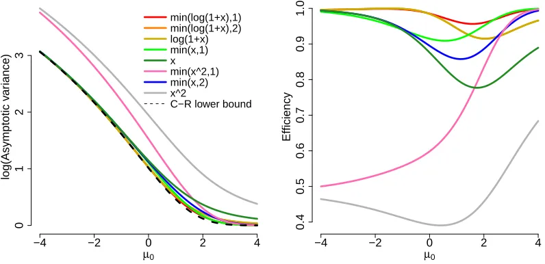
Figure 1 plots the asymptotic variance of ˆµh from Example 3.1, with σ = 1 known.
Efficiency as measured by the Cram´er-Rao lower bound divided by the asymptotic variance
is also shown. We see that two truncated versions of log(1 +x) have asymptotic variance
close to the Cram´er-Rao bound. This asymptotic variance is also reflective of the variance
for smaller finite samples.
Figure 2 is the analog of Figure 1 for ˆσ2h from Example 3.2 withµ= 0.5 known. While
the specifics are a bit different the benefits of using bounded or slowly growingh are again
clear. We note that whenσ is small, the effect of truncation to the positive part of the real
line is small.
In both plots we order/color the curves based on their overall efficiency, so they have different colors in one from the other, although the same functions are presented. For all functions presented here (A1)–(A2) and (C1)–(C2) are satisfied.
4. Regularized Generalized Score Matching
In high-dimensional settings, when the numberr of parameters to estimate may be larger
than the sample sizen, it is hard, if not impossible, to estimate the parameters consistently
without turning to some form of regularization. More specifically, for exponential families,
condition (C1) in Section 3 fails when r > n. A popular approach is then the use of `1
regularization to exploit possible sparsity.
Let the data matrix x∈Rn×m comprisen i.i.d. samples from distribution P0. Assume
P0 has densityp0 belonging to an exponential family P+ ≡ {pθ :θ ∈Θ}, where Θ⊆Rr.
Adding an`1 penalty to (10), we obtain the regularized generalized score matching loss
1 2θ
>Γ(x)θ−g(x)>θ+λkθk
1 (14)
as in Lin et al. (2016). The loss in (14) involves a quadratic smooth part as in the familiar
−4 −2 0 2 4
0
1
2
3
µ0
log(Asymptotic v
ar
iance)
min(log(1+x),1) min(log(1+x),2) log(1+x) min(x,1) x min(x^2,1) min(x,2) x^2
C−R lower bound
−4 −2 0 2 4
0.4
0.5
0.6
0.7
0.8
0.9
1.0
µ0
Efficiency
Figure 1: Log of asymptotic variance and efficiency with respect to the Cram´er-Rao bound
for ˆµh (σ2 = 1 known).
0 2 4 6 8 10
−5
0
5
10
σ0
log(Asymptotic v
ar
iance)
min(x,1) min(x,2) min(x^2,1) min(log(1+x),1) log(1+x) min(log(1+x),2) x
x^2
C−R lower bound
0 2 4 6 8 10
0.5
0.6
0.7
0.8
0.9
1.0
σ0
Efficiency
Figure 2: Log of asymptotic variance and efficiency with respect to the Cram´er-Rao bound
the regularized loss in (14) is not guaranteed to be bounded unless the tuning parameter
λ is sufficiently large—a problem that does not occur in lasso. We note that here, and
throughout, we suppress the dependence on the dataxforΓ(x),g(x) and derived quantities.
For a more detailed explanation, note that that by (11),Γ=H>Hfor someH∈Rnm×r.
In the high-dimensional case, the rank of Γ, or equivalentlyH, is at most nm < r. Hence,
Γ is not invertible and g does not necessarily lie in the column span ofΓ. Let Ker(Γ) be
the kernel ofΓ. Then there may exist ν ∈Ker(Γ) withg>ν 6= 0. In this case, if
0≤λ < sup
ν∈Ker(Γ)
|g>ν|/kνk1,
there existsν ∈Ker(Γ) with 12ν>Γν = 0 and−g>ν+λkνk1<0. Evaluating atθ(a) =a·ν
for scalara >0, the loss becomesa −g>ν +λkνk1
, which is negative and linear ina, and
thus unbounded below. In this case no minimizer of (14) exists for small values ofλ. This
issue also exists for the estimators from Zhang and Zou (2014) and Liu and Luo (2015), which correspond to score matching for GGMs. We note that in the context of estimating
the interaction matrix in pairwise models, r =m2; thus, the condition nm < r reduces to
n < m, orn < m+ 1 when bothKand η are estimated.
To circumvent the unboundedness problem, we add small values γ`>0 to the diagonal
entries of Γ, which become Γ`,`+γ`, ` = 1, . . . , r. This is in the spirit of work such as
Ledoit and Wolf (2004) and corresponds to an elastic net-type penalty (Zou and Hastie,
2005) with weighted `2 penalty Pr`=1γ`θ`2. After this modification, Γ is positive definite,
our regularized loss is strongly convex in θ, and a unique minimizer exists for all λ ≥ 0.
For the special case of truncated GGMs, we will show that a result on consistent estimation
holds if we chooseγ` =δ0Γ`,` for a suitably small constant δ0 >0, for which we propose a
particular choice to avoid tuning. This choice ofγ` depends on the data throughΓ`,`.
Definition 8 For γ∈Rr
+\{0}, letΓγ ≡Γ+ diag(γ). The regularized generalized h-score
matching estimator with tuning parameterλ≥0 and amplifier γ is the estimator
ˆ
θ ∈argmin
θ∈Θ
ˆ
Jh,λ,γ(θ)≡argmin θ∈Θ
1 2θ
>Γ
γ(x)θ−g(x)>θ+λkθk1. (15)
In the case where γ= (δ−1)diag(Γ) for some δ >1, we also call δ themultiplier. We
note that ˆθ from (15) is apiecewise linear function of λ(Lin et al., 2016).
5. Score Matching for Graphical Models for Non-negative Data
In this section we apply our generalized score matching estimator to a general class of graphical models for non-negative data.
5.1. A General Framework of Pairwise Interaction Models
We consider the class of pairwise interaction power models with density introduced in (1). We recall the form of the density:
pη,K(x)∝exp
− 1
2ax
a>
Kxa+η>x
b−1 m
b
where a and b are known constants, and the interaction matrix K and the vector η are
parameters. Whenb= 0, we use the convention that x00−1 ≡logx and apply the logarithm
element-wise. Our focus will be on the interaction matrixKthat determines the conditional
independence graph through its support S(K) ≡ {(i, j) : κij 6= 0}. However, unless η is
known or assumed to be zero, we also need to estimateη as a nuisance parameter. In the
case where we assumeη ≡0 is known (i.e. the linear part (xb−1m)/b is not present), we
call the distribution (and the corresponding estimator) acentered distribution (estimator),
in contrast to the general case termednon-centered when we assume η6=0 or unknown.
We first give a set of sufficient conditions for the density to be valid, i.e., the right-hand side of (16) to be integrable. The proof is given in Appendix A.3.
Theorem 9 Define conditions
(CC1) K is strictly co-positive, i.e., v>Kv >0 for all v∈Rm +\{0}; (CC2) 2a > b >0;
(CC3) a >0, b= 0, and ηj >−1 for j= 1, . . . , m(η −1m).
In the non-centered case, if (CC1) and one of (CC2) and (CC3) holds, then the function on the right-hand side of (16) is integrable overRm+. In the centered case, (CC1) anda >0 are sufficient.
We emphasize that (CC1) is a weaker condition than positive definiteness. Criteria for
strict co-positivity are discussed in V¨aliaho (1986).
5.2. Implementation for Different Models
In this section we give some implementation details for the regularized generalizedh-score
matching estimator defined in (15) applied to the pairwise interaction models from (16).
We again letΨ≡ K>,η>∈R(m+1)×m. The unregularized loss is then
ˆ
Jh(P) =
1
2vec(Ψ)
>Γ(x)vec(Ψ)−g(x)>vec(Ψ).
The general form of the matrix Γ and the vector g in the loss were given in equations
(10)–(12). Here Γ∈R(m+1)m×(m+1)m is block-diagonal, with thej-th
R(m+1)×(m+1) block
Γj(x)≡
Γ11,j Γ12,j Γ>12,j Γ22,j
(17)
≡ 1
n
n
X
i=1
hj
Xj(i)Xj(i)2a−2X(i)aX(i)a> −hj
Xj(i)Xj(i)a+b−2X(i)a
−hj
Xj(i)
Xj(i)a+b−2X(i)a> hj
Xj(i)
Xj(i)2b−2
= 1
ny
>y, y≡h−(p
hj(Xj)◦Xaj−1)◦xa
p
hj(Xj)◦Xbj−1
i
∈Rn,m+1, (18)
where the◦product between a vector and a matrix means an elementwise multiplication of
Furthermore, g ≡
vec(g1)
g2
∈ R(m+1)m, where g
1 and g2 correspond to each entry of K
and η, respectively. The j-th column ofg1 ∈Rm×m, written as g1,j(x), is
1 n
n
X
i=1
h0j
Xj(i)
Xj(i)a−1+ (a−1)hj
Xj(i)
Xj(i)a−2
X(i)a+ahj
Xj(i)
Xj(i)2a−2ej,m,
whereej,m is the m-vector with 1 at thej-th position and 0 elsewhere, and the j-th entry
of g2 ∈Rm is
g2,j =
1 n
n
X
i=1
−h0j
Xj(i)
Xj(i)b−1−(b−1)hj
Xj(i)
Xj(i)b−2.
These formulae also hold for b = 0 since Γ and g only depend on the gradient of the
log density, and d(xbd−x1)/b =xb−1 also holds forb= 0. In the centered case where we know
η0 ≡0, we only estimateK∈Rm×m, andΓ∈
Rm 2×m2
is still block-diagonal, with thej-th
block being theΓ11,j submatrix in (17), whileg is just vec(g1). Sincebonly appears in the
η part of the density, the formulae only depend on ain the centered case.
We emphasize that it is indeed necessary to introduce amplifiers γ 0 or a multiplier
δ >1 in addition to the`1 penalty. It is clear from (18) that rank(Γj)≤min{n, m+ 1}(or
min{n, m} if centered). Thus, Γ is non-invertible when n≤m (or n < m if centered) and
g need not lie in its column span.
We claim that including amplifiers/multipliers for the submatricesΓ11,j only is sufficient
for unique existence of a solution for all penalty parameters λ ≥ 0. To see this, consider
any nonzero vector ν ∈Rm+1. Partition it asν ≡(ν
1,ν2) withν1 ∈Rm. Let Γj,γ be our
amplified version of the matrix Γj from (21), so
Γj,γ =
Γ11,j+ diag(γ1, . . . , γm) Γ12,j Γ>12,j Γ22,j
.
AsΓj itself is positive semidefinite, we find that if at least one of the firstm entries ofν is
nonzero then
ν>Γj,γν ≥ ν>Γjν+
m
X
k=1
νk2γk ≥
m
X
k=1
νk2γk > 0.
If only the last entry of ν is nonzero then
ν>Γj,γν = νm2+1Γ22,j > 0
almost surely; recall that Γ22,j= n1Pni=1hj
Xj(i)
Xj2b−2. We conclude thatΓj,γ (and thus
the entire amplified Γ) is a.s. positive definite, which ensures unique existence of the loss
minimizer.
Given the formulae forΓandg, one adds the`1 penalty onΨto get the regularized loss
(24). Our methodology readily accommodates two different choices of the penalty parameter
λforK and η. This is also theoretically supported for truncated GGMs, since if the ratio
easily modified by replacing η by (λη/λK)η. To avoid picking two tuning parameters, one
may also choose to remove the penalty on η altogether by profiling out η and solve for
ˆ
η≡Γ−221g2−Γ>12vec(Kˆ), with Kˆ the minimizer of the profiled loss ˆ
Jh,λ,γ,profile(K)≡
1
2vec(K)
>
Γγ,11.2vec(K)−(g1−Γ12Γ −1 22g2)
>
vec(K) +λkKk1, (19)
where the Schur complement Γγ,11.2 ≡ Γγ,11−Γ12Γ−221Γ
>
12 is a.s. positive definite such
that the profiled estimator exists a.s. for all λ≥0. This profiled approach corresponds to
choosingλη/λK = 0. A detailed theoretical analysis of the profiled estimator is beyond the
scope of this paper, however. We note that in the other extreme, with λη/λK = +∞, the
non-centered estimator reduces to the estimator from the centered case.
Example 5.3 The truncated normal model comprises the density
pµ,K(x) ∝ exp
−1
2(x−µ)
>
K(x−µ)
1[0,∞)m(x). (20)
This corresponds to (16) with a=b= 1, andη=Kµ. Thej-th(m+ 1)×(m+ 1) block of Γ(x) is
1 n
x>diag(hj(Xj))x −x>hj(Xj)
−hj(Xj)>x hj(Xj)>1n
. (21)
Partitioning the vector g(x) into m subvectors gj(x) ∈ Rm+1, where the entries of g j(x) correspond to column Ψj, the k-th entry of gj(x) is
gjk(x)≡
1 n Pn
i=1h0j
Xj(i)
Xk(i) if k≤m, k6=j,
1 n
Pn
i=1h 0
j
Xj(i)Xk(i)+hj
Xj(i) if k=j,
−n1Pn
i=1h0j
Xj(i) if k=m+ 1.
(22)
Example 5.4 The exponential square-root graphical model in Inouye et al. (2016) has
pη,K(x)∝exp
−√x>K√x+ 2η>√x
1[0,∞)m(x),
which corresponds to (16) witha=b= 1/2. We refer to this as the exponential model. In this case, the j-th R(m+1)×(m+1) block ofΓ is
Γj(x)≡
1 n n X i=1 hj Xj(i) Xj(i)
−pX(i)
1 !
−pX(i)
>
,1
and g= vec(g0), where the j-th column of g0∈R(m+1)×m is
gj(x)≡ 1
n
n
X
i=1
2h0j
Xj(i)
Xj(i)−hj
Xj(i)
2Xj(i)3/2
p
X(i)
−1
!
+ hj
Xj(i)
2Xj(i)
Example 5.5 If a= 1/2 and b= 0, then (16) becomes
pη,K(x)∝exp
−√x>K√x+η>log(x)
1(0,∞)m(x). (23)
If Kis diagonal in this case, then X ∼pη,K has independent entries with Xj following the gamma distribution with rate κjj and shape ηj + 1, which gives an intuition for condition (CC3)ηj >−1in Theorem 9. We can thus view (23) as a multivariate gamma distribution with pairwise interactions among the covariates, and call this the gamma model. For this model, the j-th block of Γ is
Γj(x)≡
1 n
n
X
i=1
hj
Xj(i) Xj(i)2
− q
Xj(i)X(i) 1
!
− q
Xj(i)X(i)
>
,1
and the part of g corresponding to Kj is
g1,j(x)≡ 1
n
n
X
i=1
2h0j
Xj(i)
Xj(i)−hj
Xj(i)
2Xj(i)3/2
p
X(i)+
hj
Xj(i)
2Xj(i)
ej,m,
while the part for ηj is
g2.j(x) =
1 n
n
X
i=1
hj
Xj(i)
Xj(i)2 −
h0j
Xj(i)
Xj(i) .
We note that the Γ11,j sub-matrix of Γj and the g1,j sub-vector of gj for the gamma
model are the same as those for the exponential model, sincea= 1/2 in both cases and the
parts involvingKin the densities are the same.
5.3. Computational Details
In the most general exponential family setting, as in Eq. (10)–(12) in Theorem 5, the time complexity for forming Γ∈Rr×r and g∈Rr isO nm(fb0(m) +r2+r(ft0(m) +ft00(m))).
Here fb0(m) is the average time complexity for calculating ∂jb(x) over j = 1, . . . , m, and
similarly ft0(m) for ∂jt`(x) and ft00(m) for ∂jjt`(x) over j = 1, . . . , m and ` = 1. . . , r. In
many applications, however, these three functions would be constant in m, thus giving an
O(nmr2) computational complexity, with the dominating term coming from the operations
fort0jt0j> inΓ sinceΓ is of dimensionr×r.
For pairwise interaction power models,r=m2and the formula above becomesO(nm5).
However, sinceΓis block-diagonal with onlym3 nonzero entries and by the special form of
t(x) =xaxa>, the true complexity is in fact O(nm3).
While the introduction of the`1penalty inevitably precludes the estimator from having a
closed-form solution and introduces non-differentiability, state-of-art numerical optimization algorithms, such as coordinate-descent (Friedman et al., 2007), can be applied for fast estimation. To speed up estimation, one can usually use warm starts using the solution
from the previous λ’s, as well as lasso-type strong screening rules (Tibshirani et al., 2012)
In our implementation for pairwise interaction models of Section 5.1 (that will become available in an R package), we optimize our loss functions with respect to a symmetric
matrix ˆK; in the non-centered case the vector ˆη is also included. We use a
coordinate-descent method analogous to Algorithm 2 in Lin et al. (2016), where in each step we
update each element of ˆKand ˆη based on the other entries from the previous steps, while
maintaining symmetry. In our simulations in Section 7 we always scale the data matrix
by column `2 norms before proceeding to estimation. Note that estimation of ˆK without
symmetry can be parallelized as the loss can be decomposed into a sum over the columns.
5.4. Choice of the Function h
In this subsection we discuss the requirements on the functionhas well as some reasonable
choices of h.
5.4.1. Requirements on h
In Section 2.2, we presented two assumptions (A1) and (A2) under which the generalized score-matching loss is valid, i.e., the integration by parts is justified and Theorem 3 holds.
In this section, we present some sufficient (and nearly necessary) requirements on h such
that (A1) and (A2) are satisfied.
Definition 10 Suppose h:Rm+ →Rm+ with h(x) = (h1(x1), . . . , hm(xm))>. We write that
h∈ Ha,b (for simplicity we omit the dependency on m) if for all j= 1, . . . , m:
i) hj is absolutely continuous in every bounded sub-interval of R+, and thus has deriva-tiveh0j a.s.;
ii) hj(x)>0 a.s. onR+;
iii) hj and h0j are both bounded by some piecewise powers of x a.s. onR+;
iv) lim
x&0+hj(x)/x q
j = 0, where q ≡
(
max{1−a,1−b} if b >0,
1−η0,j if b= 0.
Theorem 11 Assume everyP in the family of distribution P+ satisfies (CC1)–(CC3) and thus has finite normalizing constants. If h∈ Ha,b, then (A1) and (A2) are satisfied.
In centered models, where η ≡ 0, we can assume b = 2a and iv) in the definition of
Ha,2a has q = 1−a. For truncated GGMs, a = b = 1, so iv) in Definition 10 is simply
limxj&0+hj(xj) = 0.
In the case of b = 0,η is an unknown parameter, and (CC3) requires each of its
com-ponent to be greater than−1. If one has prior information onηor restricts the parameter
space for η, the requirement reduces to hj(xj) = o(x
1−η0,j
j ) as xj & 0+. Otherwise, it
suffices to require hj(xj) =o(x2j). Note that this is only a condition forxj & 0+, and the
globally quadratic behavior of hj(xj) = x2j from the original score matching is not needed
5.4.2. Reasonable Choices of h
Assume a common univariate h for all components in h. Inspired by Theorem 11, we
consider h that behaves like a power of x both as x % +∞ and as x & 0+. Since the
requirements on the two tails are separate, we can choosehto be a piecewise defined function
that joins two powers with possibly different degrees. In other words,h(x) = min(xp1, cxp2)
for some powers p1 ≥ p2 ≥ 0 and constant c > 0. Only one constant c is required since
generalized score matching is invariant to scaling of h. In determining the exact power of
p1 we have the following considerations:
a) In the centered case:
(i) (A1) and (A2): Theorem 11 requires that p1≥1−a.
(ii) “Controlled Γ and g for xa”: We propose avoiding poles at the origin for the
entries ofΓandg. The formula forΓ11in (18) shows that to this endph(x)xa−1
needs to have a non-negative degree . This requires p1 ≥ 2−2a. The formula
forg1 similarly shows thath0(x)xa−1,h(x)xa−2 and h(x)x2a−2 all need to have
a non-negative degree for small x. This requires p1 ≥2−a.
b) In the non-centered case, in addition to (i) and (ii),
(iii) (A1) and (A2): Theorem 11 requires p1 ≥ max{1−a,1 −b} for b > 0, or
1−minjη0,j forb= 0.
(iv) “ControlledΓand gforxb”: From the definition ofΓ22and g2 and by the same
reasoning as above,ph(x)xb−1,h0(x)xb−1 andh(x)xb−2 need to be non-negative
powers of x, thus requiring p1 ≥max{2−b,2−2b}= 2−b.
The choice of p2, is only relevant for large data points. Our main consideration is then
merely how well Γ andg concentrate on their true population values (Theorem 13). From
this perspective, our intuition is that p2 should be chosen small so that the tails of the
distributions of the entries of Γ and g are well-behaved. Thus, we can choose p2 = 0, in
which caseh(x) = min(xp1, c) is a truncated power.
5.5. Tuning Parameter Selection
By treating the unpenalized loss (i.e.,λ= 0,γ= 0) as a negative log-likelihood, we may use
the extended Bayesian Information Criterion (eBIC) to choose the tuning parameter (Chen and Chen, 2008; Foygel and Drton, 2010). Consider the centered case as an example. Let
ˆ
Sλ ≡ {(i, j) : ˆκijλ 6= 0, i < j}, where ˆKλ be the estimate associated with tuning parameter
λ. The eBIC is then
eBIC(λ) =−nvec( ˆK)>Γ(x)vec( ˆK) + 2ng(x)>vec( ˆK) +|Sˆλ|logn+ 2 log
p(p−1)/2 |Sˆλ|
,
where ˆKcan be either the original estimate associated withλ, or a refitted solution obtained
by restricting the support to ˆSλ.
term in the above display which can be motivated by a prior distribution under which the number of edges in the conditional independence graph is uniformly distributed; see also
˙
Zak-Szatkowska and Bogdan (2011) and Barber and Drton (2015).
6. Theory for Graphical Models
In our regularized generalized score matching framework, we introduced the amplifiers/ multipliers to address the inexistence problem. We also proposed using a general function
h in place of x2 as a means to improve estimation accuracy. This section provides a
theoretical analysis of these two aspects.
In Section 6.1, we present the theory for our regularized generalized score matching estimators for general pairwise interaction models before going into the details for the special cases of (truncated) GGMs. Next, we show that a specific choice of amplifiers/multipliers yields consistent estimation without the need for tuning. This point is important even in the
case of Gaussian models on all ofRm. Therefore, in Section 6.2 we digress from non-negative
data and consider the original score matching of Hyv¨arinen (2005) for centered Gaussian
distributions. Finally, in Section 6.3, we derive probabilistic results for ˆΨbased on Theorem
13, justifying the benefits of using a general boundedhoverx2 in the non-negative setting.
As the most important models from the class of pairwise interaction power models overRm+,
we only treat truncated GGMs since they have the most tractable concentration bounds;
this case also provides a comparison to Corollary 2 in Lin et al. (2016), which usesx2.
6.1. Theory for Pairwise Interaction Models
The graphical models we treat are parametrized by the interaction matrixKand the
coeffi-cientsη on (xb−1m)/b. It is convenient to accommodate this setting with a matrix-valued
parameterΨ∈Rr1×r2 (in place of θ) and specify our regularized h-score matching loss as
ˆ
Jh,λ,γ(Ψ)≡ argmin Ψ∈Rr1×r2
1
2vec(Ψ)
>Γ
γ(x)vec(Ψ)−g(x)>vec(Ψ) +λkΨk1. (24)
In the non-centered case we thus take Ψ= [K,η]>∈Rm(m+1)×m. In the centered case,
Ψis simply them×minteraction matrixK. Following related prior work such as Lin et al.
(2016), for ease of proof we allow the matrix K to be nonsymmetric, which allows us to
decouple optimization over the different columns of KorΨ, while in our implementations
we ensure that Kis symmetric.
Definition 12 Let Γ0 ≡E0Γ(x) and g0 ≡E0g(x) be the population versions of Γ(x) and
g(x) under the distribution given by a true parameter matrix Ψ0. The support of a matrix Ψis S(Ψ)≡ {(i, j) :ψij 6= 0}, and we let S0 =S(Ψ0). For a matrix Ψ0, we definedΨ0 to
be the maximum number of non-zero entries in any column, andcΨ0 ≡ |||Ψ0|||∞,∞. Writing Γ0,AB for the A×B submatrix of Γ0, we define
cΓ0 ≡ |||(Γ0,S0S0)
−1|||
∞,∞. (25)
Finally, Γ0 satisfies the irrepresentability condition with incoherence parameter α∈(0,1]
and edge set S0 if
|||Γ0,Sc
0S0(Γ0,S0S0)
−1|||
Our analysis of the regularized generalized h-score matching estimator builds on the following theorem taken from Lin et al. (2016, Theorem 1).
Theorem 13 SupposeΓ0hasΓ0,S0S0 invertible and satisfies the irrepresentability condition
(26) with incoherence parameterα ∈(0,1]. Assume that
kΓγ(x)−Γ0k∞< 1, kg(x)−g0k∞< 2, (27)
with dΨ01 ≤α/(6cΓ0). If
λ > 3(2−α)
α max{cΨ01, 2},
then the following holds:
(a) The regularized generalized h-score matching estimator Ψˆ minimizing (24) is unique, with supportSˆ≡S( ˆΨ)⊆S0, and satisfies
kΨˆ −Ψ0k∞≤ cΓ0
2−αλ.
(b) If
min
1≤j<k≤m|Ψ0,jk|>
cΓ0
2−αλ,
thenSˆ=S0 and sign( ˆΨjk) = sign(Ψ0.jk) for all(j, k)∈S0.
This result is deterministic, and the improvement of our generalized estimator over the one in Lin et al. (2016) is in its probabilistic guarantees, as shown for truncated GGMs in Theorems 16 and 17 in Section 6.3. Before going into these examples, we state a general corollary.
Corollary 14 Under the assumptions of Theorem 13, the matrix Ψˆ minimizing (24) sat-isfies
kΨˆ −Ψ0kF ≤
cΓ0
2−αλ
p
|S0| ≤
cΓ0
2−αλ
p dΨ0m,
kΨˆ −Ψ0k2 ≤
cΓ0
2−αλmin(
p
|S0|, dΨ0).
6.2. Revisiting Gaussian Score Matching
In this section we consider estimating the inverse covariance matrixKof a centered Gaussian
distribution N(0,K), which of course has density proportional to (2) on all ofRm. As shown,
e.g., in Example 1 of Lin et al. (2016), the`1-regularized score matching loss then takes the
form
1
2tr(KKxx
>)−tr(K) +λkKk
1, (28)
which can be written as (14) with θ= vec(K), Γ= diag(xx>, . . . ,xx>) andg = vec(Im).
Thus, in general, the kernel ofΓ need not be orthogonal to g, and for λsmall the loss can
be unbounded below as discussed above. Hence, an amplifier/multiplier on the diagonals
Theorem 15 Suppose the data matrix x holdsn i.i.d. copies ofX ∼N(0,K0). Adopt the amplifying in Section 4 and redefine the loss in (28) as
1
2tr(KKG)−tr(K) +λkKk1, Gjk = (xx
>)
jk 1{j6=k}+ (δ−1)1{j=k}
, (29)
where 1 < δ < 2−1 + 80plogm/n
−1
. Let Kˆ be the resulting estimator. Let c∗ ≡
12800 (maxjΣ0,jj)2 and c1 = 4cΓ0/α. If for some τ >2, the regularization parameter and
the sample size satisfy
λ >(2cK0(2−α)
p
c∗(τlogm+ log 4)/n)/α,
n >max(c∗c21dK2 0,2)(τlogm+ log 4),
thenkKˆ −K0k∞≤
cΓ0
2−αλwith probability1−m 2−τ.
In Corollary 1 of Lin et al. (2016) the same results were shown withc∗ ≡3200 (maxjΣ0,jj)2
when a unique minimizer exists, but the existence was not guaranteed.
6.3. Generalized Score Matching for Truncated GGMs
Next, we provide theory for the regularized generalized h-score matching estimator ˆΨ in
the special case of truncated GGMs. Again, assume a commonh for all components inh.
Theorem 16 Suppose the data matrix x holds n i.i.d. copies of X ∼ TN(0,K0), where the mean parameter is known to be zero. Assume that h ∈ H1,1 and that 0 ≤ h ≤ M,
0≤h0 ≤M0 a.s. for constants M, M0, and choose γ= (δ−1)diag(Γ) with
1< δ < C(n, m)≡2−1 + 4emax{6 logm/n,p6 logm/n}−1.
Suppose that the Γ0,S0S0 block of Γ0 is invertible and Γ0 satisfies the irrepresentability
condition (26) with α ∈ (0,1] and true edge set S0. Define cX ≡ 2 maxj
2
q
(K−01)jj +
√ eE0Xj
. If for τ >3 the sample size and the regularization parameter satisfy
n >O τlogmmax
(
M2c2Γ0c4Xd2K0
α2 ,
M cΓ0c
2 XdK0
α
)!
, (30)
λ >O "
(M cK0c
2 X +M
0
cX+M)
r
τlogm
n +
τlogm
n !#
, (31)
then the following statements hold with probability 1−m3−τ:
(a) The regularized generalized h-score matching estimator Kˆ that minimizes (24) is unique, has its support included in the true support,Sˆ≡S( ˆK)⊆S0, and satisfies
kKˆ −K0k∞≤
cΓ0
|||Kˆ −K0|||F ≤
cΓ0
2−αλ
p |S0|,
|||Kˆ −K0|||2 ≤ cΓ0
2−αλmin(
p
|S0|, dK0),
where cΓ0 is defined in (25).
(b) Moreover, if
min
j,k:(j,k)∈S0
|κ0,jk|>
cΓ0
2−αλ,
thenSˆ=S0 and sign(ˆκjk) = sign(κ0,jk) for all (j, k)∈S0.
The theorem is proved in Appendix A.4, where details on the dependencies on constants
are provided. A key ingredient of the proof is a tail bound on kΓγ −Γ0k∞, which features
products of the Xj(i)’s. In Lin et al. (2016), the products are up to fourth order. Using
bounded h, our products automatically calibrates to a quadratic polynomial when the
observed values are large, and resort to higher moments only when they are small. This leads to improved bounds and convergence rates, underscored in the new requirement on
the sample size n, which should be compared ton≥ O(d2K0(logmτ)8) in Lin et al. (2016).
For the non-centered case, by definition, cΨ0 ≡ |||Ψ0
>|||
∞,∞ ≤ cK0 +kη0k∞, dΨ0 ≤
dK0+1. The proof given for Theorem 16 goes through again here, and we have the following
consistency results.
Theorem 17 Suppose the data matrix holds n i.i.d. copies of X ∼TN(µ0,K0). Assume that h ∈ H1,1 and that 0 ≤ h ≤ M, 0 ≤ h0 ≤ M0 a.s. for constants M, M0. Let γ be a vector of amplifiers that are non-zero only for the diagonal entries of the matrices Γ11,j, amplifying those by(δ−1)diag(Γ11,j) with
1< δ < C(n, m)≡2−1 + 4emax{6 logm/n,p6 logm/n}−1.
Suppose further that Γ0,S0S0 is invertible and satisfies the irrepresentability condition (26)
with α ∈ (0,1]. Define cX ≡ 2 maxj
2
q
(K−01)jj+
√ eE0Xj
. Suppose for τ > 3 the
sample size and the regularization parameter satisfy
n >O τlogmmax
( M2c2Γ
0,Ψ0c
4 Xd2Ψ0
α2 ,
M cΓ0,Ψ0c
2 XdΨ0
α
)!
, (32)
λ >O "
(M cΨ0c
2
X +M0cX+M)
r
τlogm
n +
τlogm
n !#
, (33)
where cΓ0,Ψ0 is cΓ0 as in (25) but with notation Ψ0 to differentiate it from the centered
case. Then the following statements hold with probability 1−m3−τ:
(a) The regularized generalized h-score matching estimator Ψˆ that minimizes (24) is unique, has its support included in the true support,Sˆ≡S( ˆΨ)⊆S0, and satisfies
kKˆ −K0k∞≤
cΓ0,Ψ0
2−αλ, kηˆ−η0k∞≤
cΓ0,Ψ0
|||Kˆ −K0|||F ≤
cΓ0,Ψ0
2−αλ
p
|S0|, |||ηˆ−η0|||F ≤
cΓ0,Ψ0
2−αλ
p |S0|,
|||Kˆ −K0|||2 ≤ cΓ0,Ψ0
2−αλmin
p
|S0|, dΨ0
, |||ηˆ−η0|||2 ≤ cΓ0,Ψ0
2−αλmin
p
|S0|, dΨ0
.
(b) Moreover, if
min
j,k:(j,k)∈S0
|κ0,jk|>
cΓ0
2−αλ and j:(mmin+1,j)∈S0
|η0,j|>
cΓ0
2−αλ,
then Sˆ = S0 and sign(ˆκjk) = sign(κ0,jk) for all (j, k) ∈ S0 and sign(ˆηj) = sign(η0j) for (m+ 1, j)∈S0.
Remark 18 The quantity cX in Theorem 17 depends on E0Xj, which in turn depends
on the structure of both µ0 and K0. If µ0,j is large compared to (K0)−jj1, then cX seems
to scale as µ0, which negatively impacts the guarantees stated in Theorem 17. However,
as in the one-dimensional case for estimation of µ0 (Example 3.1), our estimator should
automatically adapt to the large mean parameter. This suggests that it might be possible
to improve our analysis involvingcX.
7. Numerical Experiments
In this section, we compare the performance of our estimator with different choices of h
to the existing approaches for pairwise interaction power models. In our simulation
exper-iments, we consider m = 100 variables and n= 80 and n = 1000 samples, corresponding
to high- and low-dimensional settings. We also tried intermediate sample sizes between
these two extremes, but found no interesting result worth reporting. For n = 80,
ampli-fication is necessary. Except in Section 7.2.2, the amplifier is set based on Theorem 16
to δ = C(n, m) = 1.8647 for truncated GGMs. The same amplifier is also used for
set-tings with other a and b. For n = 1000, we consider δ = 1, i.e., no amplification, and
δ =C(n, m) = 1.6438 (again, based on Theorem 16). Throughout, we assume a common
univariate h for all components inh.
7.1. Structure of K
The underlying interaction matrices are selected as follows: Proceeding as in Section 4.2 of Lin et al. (2016), the graph is chosen to have 10 disconnected subgraphs, each containing
m/10 nodes. Thus,K0 is block-diagonal. In each block, each lower-triangular element is set
to 0 with probability 1−πfor someπ∈(0,1), and is otherwise drawn from Uniform[0.5,1].
The upper triangular elements are determined by symmetry. The diagonal elements ofK0
are chosen as a common positive value such that the minimum eigenvalue ofK0 is 0.1.
We generate 5 different true precision matrices K0, and run 10 trials with each of these
precision matrices. Forn= 1000, we choose π= 0.8, which is in accordance with Lin et al.
(2016). For n = 80, we set π = 0.2. This way n/(d2K0logm) is roughly constant; recall
Theorems 16 and 17 for truncated GGMs.
In Appendix C, we report results on Erd¨os-R´enyi graphs, which lead to similar
7.2. Truncated GGMs
Given our focus on truncated GGMs and their relevance in graphical modeling applications, we start with experiments for these models.
7.2.1. Choice of h
Our estimator requires choosing a function h : Rm+ → Rm+. For simplicity, we will always
specifyh(x) = (h(x1), . . . , h(xm)) for a single non-decreasing univariate functionh:R+ →
R+, i.e. all coordinates share the same hfunction.
As previously explained, h ∈ Ha,b is a sufficient condition for assumptions (A1)-(A2),
as well as (C1)-(C2) in the case of unregularized estimators. Only in the proofs of our
theoretical guarantees in Section 6 for truncated GGMs, did we require h to be bounded
and to have bounded derivatives. As motivated by the discussion in Section 5.4.2, we
consider truncated and untruncated powers, min(x, c) and x (since 2−a= 2−b= 1); we
evaluate this choice by contrasting them with powersx1.5 andx2. We also explore functions
like log(1 +x) that seem natural and are linear near 0. In particular, we make a further
comparison to functions linear near 0 with a finite asymptote asx%+∞but differentiable
everywhere: MCP- (Fan and Li, 2001) and SCAD-like (Zhang, 2010) functions defined
below. The results we report are based on selections of best performing choices of h.
SCAD(x;λ, γ)≡
λx if 0≤x≤λ,
2γλx−x2−λ2
2(γ−1) ifλ < x < γλ,
λ2(γ+1)
2 ifx≥γλ;
MCP(x;λ, γ)≡
(
λx−x2
2γ if 0≤x≤γλ, 1
2γλ
2 ifx > γλ.
We do not observe any clear relationship between features such as convexity,
differen-tiability or the slope of h at 0, and performance of the estimator. Nonetheless, for many
choices of rather simple functions h, our estimator provides a significant improvement over
existing methods. In particular, mosth functions that behave linearly for small x, namely
log(1 +x) and x and their truncations, and additionally MCP and SCAD, always perform
better thanx1.5 and x2. This agrees with our discussion in Section 5.4.2, where 2−a= 1
is a reasonable choice of the power for smallx; also see Section 7.3. However, we conclude
that there is no real gain from making the function smoother by using MCP or SCAD.
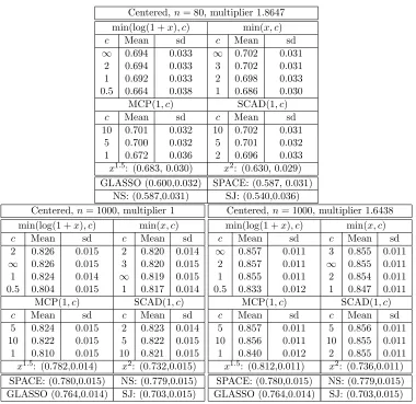
Truncated Centered GGMs: For data from a truncated centered Gaussian distribution,
we compare our generalized score matching estimator with various choices of h, to SpaCE
JAM (SJ, Voorman et al., 2014), which estimates graphs using additive models for
condi-tional means, a pseudo-likelihood methodSPACE (Peng et al., 2009) in the reformulation
of Khare et al. (2015), graphical lasso (GLASSO, Yuan and Lin, 2007; Friedman et al.,
2008), the neighborhood selection estimator (NS) of Meinshausen and B¨uhlmann (2006),
and nonparanormal SKEPTIC (Liu et al., 2012) with Kendall’s τ. Recall that the choice
of h(x) =x2 corresponds to the estimator from Lin et al. (2016).
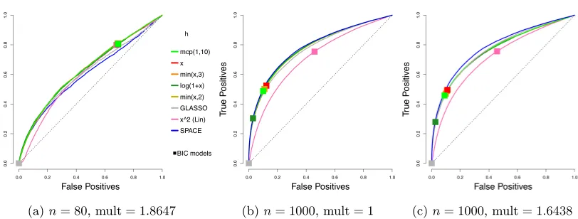
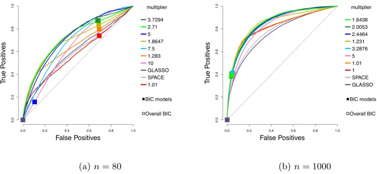
The ROC (receiver operating characteristic) curves for different estimators are shown
in Figure 3 on Page 26. Each plotted curve corresponds to the average of 50 ROC curves, where the averaging is based on the vertical averaging from Algorithm 3 in Fawcett (2006),
and is mean AUC-preserving. The x and y axes of each ROC curve represent the false
Centered,n= 80, multiplier 1.8647
min(log(1 +x), c) min(x, c)
c Mean sd c Mean sd
∞ 0.694 0.033 ∞ 0.702 0.031 2 0.694 0.033 3 0.702 0.031 1 0.692 0.033 2 0.698 0.033 0.5 0.664 0.038 1 0.686 0.030
MCP(1, c) SCAD(1, c)
c Mean sd c Mean sd
10 0.701 0.032 10 0.702 0.031 5 0.700 0.032 5 0.701 0.032 1 0.672 0.036 2 0.696 0.033 x1.5: (0.683, 0.030) x2: (0.630, 0.029) GLASSO (0.600,0.032) SPACE: (0.587, 0.031)
NS: (0.587,0.031) SJ: (0.540,0.036) Centered,n= 1000, multiplier 1
min(log(1 +x), c) min(x, c)
c Mean sd c Mean sd
2 0.826 0.015 2 0.820 0.014
∞ 0.826 0.015 3 0.820 0.015 1 0.824 0.014 ∞ 0.819 0.015 0.5 0.804 0.015 1 0.817 0.014
MCP(1, c) SCAD(1, c)
c Mean sd c Mean sd
5 0.824 0.015 2 0.823 0.014 10 0.822 0.015 5 0.822 0.015 1 0.810 0.015 10 0.821 0.015 x1.5: (0.782,0.014) x2: (0.732,0.015) SPACE: (0.780,0.015) NS: (0.779,0.015) GLASSO (0.764,0.014) SJ: (0.703,0.015)
Centered,n= 1000, multiplier 1.6438 min(log(1 +x), c) min(x, c)
c Mean sd c Mean sd
∞ 0.857 0.011 3 0.855 0.011 2 0.857 0.011 ∞ 0.855 0.011 1 0.855 0.011 2 0.854 0.011 0.5 0.833 0.012 1 0.847 0.011
MCP(1, c) SCAD(1, c)
c Mean sd c Mean sd
5 0.857 0.011 5 0.856 0.011 10 0.856 0.011 10 0.855 0.011 1 0.840 0.012 2 0.855 0.011 x1.5: (0.812,0.011) x2: (0.736,0.011) SPACE: (0.780,0.015) NS: (0.779,0.015) GLASSO (0.764,0.014) SJ: (0.703,0.015)
Table 1: Mean and standard deviation of areas under the ROC curves (AUC) using different
estimators in the centered setting, withn= 80 and multiplier 1.8647, orn= 1000
and multiplier 1 and 1.6438. Methods include our estimator with different choices
of h, GLASSO, SPACE, neighborhood selection (NS), and Space JAM (SJ).
FPR≡ |Sˆoff\S0,off| m(m−1)− |S0,off|
and TPR≡ |Sˆoff∩S0,off|
|S0,off|
,
whereS0,off≡ {(i, j) :i6=j∧κ0,ij 6= 0}, and ˆSoff≡ {(i, j) :i=6 j∧κˆij 6= 0}.
To reduce clutter, we only report the results for the top performing competing methods. In particular, results for nonparanormal SKEPTIC are omitted, as the method always performs the worst in our experiments. The corresponding means and standard deviations
of AUCs (areas under the curves) over 50 curves are given in Table 1.
Looking at the mean AUCs, with the standard deviations in mind, all choices of h
considered here perform better thanh(x) =x2from Hyv¨arinen (2007) and Lin et al. (2016)
and the competing methods. The results for n = 1000 in Table 1 also show that the
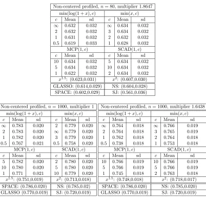
Truncated Non-Centered GGMs: We generate data from a truncated non-centered
Gaus-sian distribution with both parametersµand Kunknown. In each trial, we form the true
K0 as in Section 7.1, and generate each component of µ0 independently from the normal
distribution with mean 0 and standard deviation 0.5.
We compare the performance of our profiled estimator based on (19), with different h
functions, but with no penalty on η ≡ Kµ, to SPACE, SpaCE JAM (SJ), GLASSO, and
neighborhood selection (NS). As before, we consider 50 trials. Representative ROC curves are plotted in Figure 4, and the corresponding AUCs are summarized in Table 2.
Non-centered profiled,n= 80, multiplier 1.8647 min(log(1 +x), c) min(x, c)
c Mean sd c Mean sd
∞ 0.632 0.032 ∞ 0.634 0.032 2 0.632 0.032 3 0.634 0.032 1 0.631 0.032 2 0.632 0.032 0.5 0.619 0.033 1 0.628 0.032
MCP(1, c) SCAD(1, c)
c Mean sd c Mean sd
10 0.634 0.032 5 0.634 0.032 5 0.634 0.032 10 0.634 0.032 1 0.622 0.032 2 0.634 0.032 x1.5: (0.623,0.031) x2: (0.607,0.030)
GLASSO: (0.614,0.029) NS: (0.604,0.028) SPACE: (0.602,0.029) SJ: (0.561,0.036)
Non-centered profiled,n= 1000, multiplier 1 min(log(1 +x), c) min(x, c)
c Mean sd c Mean sd
∞ 0.783 0.020 2 0.779 0.020 2 0.783 0.020 ∞ 0.779 0.020 1 0.782 0.020 3 0.779 0.020 0.5 0.767 0.021 0.5 0.758 0.020
MCP(1, c) SCAD(1, c)
c Mean sd c Mean sd
5 0.782 0.020 2 0.780 0.020 10 0.780 0.020 5 0.780 0.020 1 0.771 0.021 10 0.779 0.020 x1.5: (0.751,0.019) x2: (0.713,0.018)
SPACE: (0.786,0.020) NS: (0.785,0.02) GLASSO (0.770,0.019) SJ: (0.720,0.019)
Non-centered profiled,n= 1000, multiplier 1.6438 min(log(1 +x), c) min(x, c)
c Mean sd c Mean sd
∞ 0.764 0.018 ∞ 0.766 0.019 2 0.764 0.018 3 0.765 0.019 1 0.762 0.018 2 0.764 0.018 0.5 0.738 0.018 1 0.753 0.018
MCP(1, c) SCAD(1, c)
c Mean sd c Mean sd
10 0.766 0.019 10 0.766 0.019 5 0.766 0.019 5 0.766 0.019 1 0.745 0.018 2 0.763 0.018 x1.5: (0.748,0.018) x2: (0.718,0.017)
SPACE: (0.786,0.020) NS: (0.785,0.020) GLASSO (0.770,0.019) SJ: (0.720,0.019)
Table 2: Mean and standard deviation of AUC using different profiled estimators in the
non-centered setting, withn= 80 and multiplier 1.8647, orn= 1000 and multipliers 1
and 1.6438. Methods include our estimator with different choices ofh, GLASSO,
(a)n= 80, mult = 1.8647 (b)n= 1000, mult = 1 (c)n= 1000, mult = 1.6438
Figure 3: Average ROC curves of our centered estimator with various choices ofh, compared
to SPACE and GLASSO, for the truncated centered GGM case;m= 100 variables
andn= 80 or 1000 samples are considered. Squares indicate average true positive
rate (TPR) and false positive rate (FPR) of models picked by eBIC with refitting for the estimator in the same color.
(a)n= 80, mult = 1.8647 (b)n= 1000, mult = 1 (c)n= 1000, mult = 1.6438
Figure 4: Average ROC curves of our non-centered profiled estimator with various choices
of h, compared to SPACE and GLASSO, for the truncated non-centered GGM
case; m = 100 variables and n = 80 or 1000 samples are considered. Squares