Cite this article as: Koy, A. (2018). Testing multi bubbles for commodity derivative markets: A study on MCX. Business and Economics Research Journal, 9(2), 291-299.
The current issue and archive of this Journal is available at: www.berjournal.com
Testing Multi Bubbles for Commodity Derivative Markets: A
Study on MCX
Ayben Koya
Abstract: Due to their volatility differences, yield differences and low correlations with equity markets, metal futures are held for diversification in the international investors’ portfolios. Beginning with dot.com bubble and following global crisis, the mutual movement of equity markets caused investors to canalize alternative investment vehicles. The study aims to investigate if there are bubbles in metal futures in The Multi Commodity Exchange of India Limited (MCX) related the period beginning from January 2010 to August 2017 for copper, lead, nickel and zinc; and March 2010 to August 2017 for aluminum in a weekly data range. Using Sup Augmented Dickey Fuller (SADF) and Generalized Sup Augmented Dickey Fuller (GSADF) tests, no evidence on bubble could be found in any metal market in the used MCX sample. The precious metal markets are out of the sample because of their relatively high volatility.
Keywords: Bubble,
Commodity Market, Metal Market, SADF, GSADF
JEL: G00, G10, G15, C58
Received: 14 December2017 Revised: 31 January 2018 Accepted: 19 March 2018
1. Introduction
For emerging economies, commodity derivatives markets have a significant place in the world economy, such as the future price determination and hedging, as well as the transfer of developed market characteristics and the development of the local financial infrastructure. On the other hand, due to their volatility differences, yield differences and low correlations with equity markets, metal futures are held for diversification in the international investors portfolios (Arouri et al., 2013; Arouri & Nguyen: 2010; Conover et al., 2010; Daskalaki & Skiadopoulos, 2011; Hammoudeh et al., 2013.) Beginning with dot.com bubble and following global crisis, the mutual movement of equity markets causes investors to canalize alternative investment vehicles such as commodity based derivatives. The growing interest of investors in commodity derivative markets may also lead prices away from the random walking process.
rapidly rising New York Stock Exchange fell 12.8 % on October 24, 1929. In late 1990s, the interest on US internet based companies stocks has been seen as rapid rise. This rapid rise collapsed in 2001. Finally, the last big bubble effected whole world economy is Mortgage crisis in 2008.
In this research investigating the existence of financial asset bubbles, commodity markets are selected as sample. The need to reduce the problems of the risky, unpredictable and unstructured agricultural industry has raised the need for the development of today's commodity derivatives. Agricultural commodity markets have a very complex mechanism involving farmers, farm owners, processors, distributors, packers, wholesalers and retailers. Moreover, it is difficult to manage risks such as extreme weather changes in agriculture, disease, natural disasters and government policies. The products that are most demanded in the world economy and whose prices are discussed are undoubtedly energy commodities. Beyond being the driving force of trade and industry, energy products that meet the needs of households are essential today in all areas of life. Firms which demand any amount of energy are at significant risk of changing prices. There are many common expectations of trading parties in the purchase and sale of any physical commodity in world trade. Expectations such as credibility, timeliness, honesty and flexibility lead to the standardization of the trade.
The use of commodity derivatives in terms of businesses leads to increased competitive advantage and profitability by using various price strategies. Enterprises using commodity derivatives in the supply of raw materials can fix production costs. Unpredictable, frequent and large fluctuations in commodity prices lead to managerial difficulties and costing problems when using these items in manufacturing enterprises, where commodity derivatives are not used without cost estimates.
Most of the transactions carried out in today's derivative markets are based on financial investment. Transferring information for future prices to all investors is an important function of futures markets. Those who collect and analyze information about the future state of the world economy will obtain returns on their investment in this information. In the absence of a futures market, investors use the information they analyze to determine the spot price for the following period. The fact that informed investors have different expectations for the future price will also cause the investor with knowledge to get a return on the market. In advanced derivative markets, the future prices are made known to all investors and the information of the investor who has knowledge is transferred to the investor who does not have knowledge.
The interest among commodity markets and commodity derivative markets encountered with speculative movements like other investment instruments over time. As exemplified in the literature part, bubbles are found in many types of commodity markets as precious metals (Baur & Glover, 2012), agriculture (Diesteldorf et al., 2016) or oil products (Su et al., 2017). In the study, the bubbles in non-precious metals as aluminum, copper, lead, nickel and zinc are detected in a growing and known commodity futures market: The Multi Commodity Exchange of India Limited (MCX). India, which have a growing share of the world economy with features such as rich natural resources, labor force, have an important place among the world's derivative markets too. National Stock Exchange of India is the 2nd derivative market with it’s 2.47 billion contracts’ volume and MCX is the 20th derivative market with it’s 0.20 billion contracts’ volume in 2017 in the world.
These selected group have the most basic inputs of industrial production. They are used in vehicles, military applications, packaging, construction, electrical-electronics, chemical and steel industries.
2. Literature
Gilbert (2009), Gutierrez (2013), Areal et al. (2014), Etienne, Irwin, and Garcia (2014), and Diesteldorf et al. (2016) test bubbles in agricultural commodity markets. Gilbert (2009) and Gutierrez (2013) find bubbles for four markets. Markets as fruits, meat and seafood have no evidence on bubbles in Areal, Balcombe and Rapsomanikis (2014). Etienne et al. (2014) find evidence on 10 of 12 commodities. Diesteldorf et al. (2016) use GSADF test to investigate the presence of bubbles in ten agriculture commodity prices. One to three bubble periods are found for six types of commodities in their study.
Gold is a valuable investment instrument, beyond being an industrial asset. Bubbles in gold prices are analyzed by Baur and McDermott (2010), Baur and Glover (2012) and Long et al. (2016). They all find evidence on the bubbles in gold prices. The other type of commodities which have importance in the world economy are energy products such as crude oil and natural gas. Su et al. (2017) find six bubbles in oil in a 21 years period ending 2016.
In recent years, studies in the literature have included bubble analysis in similar metal market samples as the sample used in this study. Ferretti et al. (2015) detect bubbles on London Metal Exchange (LME) for six non-ferrous metal prices. In another study, the global iron ore prices beginning from 1980 to 2016 are analyzed by GSADF in Su et al. (2017). Four different bubbles in the years 2005, 2006, 2007 and 2008 are found in the model.
3. Data and Model
MCX is a commodity derivatives exchange in India which started operations in November 2003. MCX is not only an important metal and energy derivatives exchange, some agricultural derivatives as black pepper, cotton, crude palm oil, and mentha oil are also have being traded. In the study, metal futures closing prices used begin from January 2010 to August 2017 (398 observations) for copper, lead, nickel and zinc; and March 2010 to August 2017 (389 observations) for aluminum in a weekly data range.
3.1. Sup Augmented Dickey Fuller Test
SADF, which is one of the right-tailed unit root tests is developed by Philips, Si and Yu (2011). The analysis allowed for a null random walk process with an asymptotically negligible drift.
yt = d𝑇−ŋ+ ∅yt − 1 + ε𝑡 , ε𝑡 ~𝑖𝑖𝑑 N (0, σ2), ∅ = 1 (1)
d = constant,
T = sample size,
ŋ › ½
The recommended empirical regression model for bubble detection in formula (1) above includes an intercept but no fitted time trend in the regression. Suppose a regression sample starts from the 𝑟1𝑡ℎ fraction
of the total sample and ends at the 𝑟12𝑡ℎ fraction of the sample, where r2 = r1 + rw and rw is the (fractional)
window size of the regression. The empirical regression model can be written as follows:
Δyt =∝𝑟1𝑟2+ 𝛽𝑟1𝑟2 𝑦𝑡−1+ ∑ki=1φ𝑟𝑖1𝑟2Δy𝑡−𝑖 + ε𝑡 (2)
k = lag order,
ε𝑡 ~𝑖𝑖𝑑 N (0, 𝛼𝑟1𝑟2
2 ),
T𝑤 = ⌊𝑇𝑟𝑤⌋ = Number of the observations in the regression
This right tailed unit root test estimates the Augmented Dickey Fuller (ADF) model repeatedly on a forward expanding sample sequence conducts a hypothesis test based on the sup value of the corresponding ADF statistic sequence.
rw = window size
window size expands from r0 to 1.
The ending point of each sample r2 is equal to rw .
The ADF statistic for a sample that runs from 0 to r2 is denoted by 𝐴𝐷𝐹0𝑟2. The SADF statistic is defined
as supr2∈[r01]𝐴𝐷𝐹0𝑟2 and is denoted by SADF (r0).
3.2. Generalized Sup Augmented Dickey Fuller Test
The GSADF test continues the idea of repeatedly running the ADF test regression (2) on a sample sequence. However, the sample sequence is broader than that of the SADF test. GSADF test allows the starting point r1 to change within a feasible range, which is from 0 to r2− r0. GSADF statistic defined to be the
largest ADF statistic over the feasible ranges for r1 and r2, and signified by GSADF(r0) (Philips et al., 2012;
2015(a); 2015 (b)).
GSADF(r0) =
sup {𝐴𝐷𝐹𝑟𝑟12}
𝑟2 𝜖[𝑟0, 1]
𝑟1 𝜖 [0, 𝑟2− 𝑟0]
(3)
Including an intercept in the regression model and the null hypothesis is a random walk without drift (i.e. dT-n with n › ½ and constant d), the limit distribution of the GSADF test statistic is can be written as
follows:
sup
{ 1
2 𝑟𝑤[𝑊(𝑟2)2 − 𝑊(𝑟1)2 − 𝑟𝑤] − ∫ 𝑊(𝑟)𝑑𝑟 [𝑊(𝑟2) − 𝑊(𝑟1)] 𝑟2
𝑟1
𝑟𝑤
1 2{𝑟
𝑤∫ 𝑊 (𝑟)2𝑑𝑟 − [∫ 𝑊 (𝑟)𝑑𝑟
𝑟2
𝑟1 ]
2 𝑟2
𝑟1 }
1 2
} 𝑟2 𝜖[𝑟0, 1]
𝑟1 𝜖 [0, 𝑟2− 𝑟0]
(4)
𝑟𝑤 = 𝑟2− 𝑟1 and W is a standard Wiener process.
The asymptotic GSADF distribution depends on the smallest window size r0. If total number of
observations (T) is small, r0 needs to be large enough to ensure there are enough observations for adequate
initial estimation. If T is large r0 can be set to be a smaller number, thus the test does not miss any opportunity
to detect an early explosive episode (Phillips, Shi and Yu (2011)).
Random and explosive processes are successfully distinguished from each other in GSADF model. It is a dominant model in analyzing speculative movements and behavioral anomalies in the market.
4. Empirical Results
The descriptive statistics of the variables are shown in Table 1. While copper price and nickel price skewed to the left (left-skewed); the prices of aluminum, lead and zinc skewed to the right (right-skewed).
The kurtosis of the futures price series of aluminum, copper and nickel are less than 3, then the series have lighter tails than a normal distribution. These series have light-tailed distributions. On the other hand, the kurtosis of the series lead futures prices and zinc futures prices are greater than 3, then they have heavier tails than a normal distribution. These series have heavier-tailed distributions.
Table 1. Descriptive Statistics
ALUMINUM COPPER LEAD NICKEL ZINC
Mean 109.8645 389.0437 119.0190 880.8905 121.6814
Median 109.2000 401.8750 118.3500 904.7000 113.3750
Maximum 131.2000 475.4000 165.1000 1312.500 200.8000
Minimum 88.65000 294.2500 75.45000 534.1000 78.30000
Std. Deviation 7.989995 45.77181 15.25960 176.5652 25.20131
Skewness 0.226836 -0.357586 0.234767 -0.100498 1.129806
Kurtosis 2.905379 2.017216 3.220565 2.316451 3.639984
Jarque-Berra 3.481091 24.49915 4.462766 8.418333 91.46416
Probability 0.175425 0.000005 0.107380 0.014859 0.000000
Sum 42737.30 154839.4 47369.55 350594.4 48429.20
Sum. Sq. Dev. 24769.93 831738.4 92442.38 12376580 252137.2
Observations 389 398 398 398 398
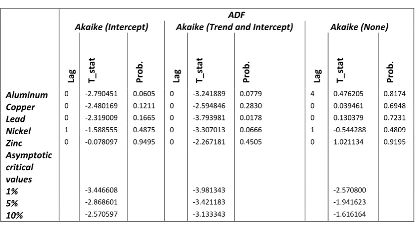
In the second step, to test the nonstationarity, the regular ADF test (Dickey Fuller, 1981), is applied to the series. The unit root tests of the variables are shown in Table 2. Except lead in the test with trend and intercept, all results in ADF tests obtain Akaike (AIC) information criteria higher than the critical values. As a result of the test, we failed to reject the hypothesis that the series are stationary.
Table 2. The Results of the Unit Root Tests ADF ADF
Akaike (Intercept) Akaike (Trend and Intercept) Akaike (None)
Lag T_stat Pro
b
.
Lag T_stat Pro
b
.
Lag T_stat Pro
b
.
Aluminum 0 -2.790451 0.0605 0 -3.241889 0.0779 4 0.476205 0.8174
Copper 0 -2.480169 0.1211 0 -2.594846 0.2830 0 0.039461 0.6948
Lead 0 -2.319009 0.1665 0 -3.793981 0.0178 0 0.130379 0.7231
Nickel 1 -1.588555 0.4875 0 -3.307013 0.0666 1 -0.544288 0.4809
Zinc 0 -0.078097 0.9495 0 -2.267181 0.4505 0 1.021134 0.9195
Asymptotic critical values
1% -3.446608 -3.981343 -2.570800
5% -2.868601 -3.421183 -1.941623
10% -2.570597 -3.133343 -1.616164
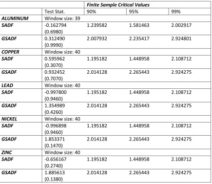
Table 3. Test Statistics for SADF and GSADF Finite Sample Critical Values
Test Stat. 90% 95% 99%
ALUMINUM Window size: 39
SADF -0.162794
(0.6980)
1.239582 1.581463 2.002917
GSADF 0.312490
(0.9990)
2.007932 2.235417 2.924801
COPPER Window size: 40
SADF 0.595962
(0.3070)
1.195182 1.448958 2.108712
GSADF 0.932452
(0.7070)
2.014128 2.265443 2.924275
LEAD Window size: 40
SADF -0.997800
(0.9460)
1.195182 1.448958 2.108712
GSADF 1.354989
(0.4260)
2.014128 2.265443 2.924275
NICKEL Window size: 40
SADF -0.996898
(0.9460)
1.195182 1.448958 2.108712
GSADF 1.853371
(0.1470)
2.014128 2.265443 2.924275
ZINC Window size: 40
SADF -0.656167
(0.2740)
1.195182 1.448958 2.108712
GSADF 1.885613
(0.1380)
2.014128 2.265443 2.924275
Critical values are based on a Monte Carlo simulation
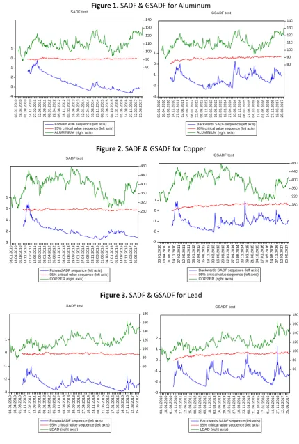
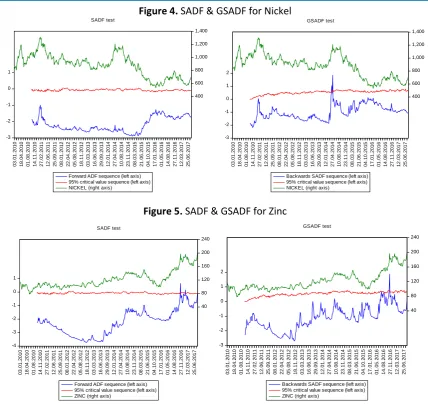
The figures 1-5 show the futures prices in green, critical values in red and the calculated sequences in blue. Generally, the areas above the red critical values of the blue line, indicate bubble possibilities.
Figure 1. SADF & GSADF for Aluminum -4 -3 -2 -1 0 1 80 90 100 110 120 130 140 03 .01 .20 10 18 .04 .20 10 01 .08 .20 10 14 .11 .20 10 27 .02 .20 11 12 .06 .20 11 25 .09 .20 11 08 .01 .20 12 22 .04 .20 12 05 .08 .20 12 18 .11 .20 12 03 .03 .20 13 16 .06 .20 13 29 .09 .20 13 12 .01 .20 14 27 .04 .20 14 10 .08 .20 14 23 .11 .20 14 08 .03 .20 15 21 .06 .20 15 04 .10 .20 15 17 .01 .20 16 01 .05 .20 16 14 .08 .20 16 27 .11 .20 16 12 .03 .20 17 25 .06 .20 17
Forward ADF sequence (left axis) 95% critical value sequence (left axis) ALUMINIUM (right axis)
SADF test -3 -2 -1 0 1 80 90 100 110 120 130 140 03 .01 .20 10 18 .04 .20 10 01 .08 .20 10 14 .11 .20 10 27 .02 .20 11 12 .06 .20 11 25 .09 .20 11 08 .01 .20 12 22 .04 .20 12 05 .08 .20 12 18 .11 .20 12 03 .03 .20 13 16 .06 .20 13 29 .09 .20 13 12 .01 .20 14 27 .04 .20 14 10 .08 .20 14 23 .11 .20 14 08 .03 .20 15 21 .06 .20 15 04 .10 .20 15 17 .01 .20 16 01 .05 .20 16 14 .08 .20 16 27 .11 .20 16 12 .03 .20 17 25 .06 .20 17
Backwards SADF sequence (left axis) 95% critical value sequence (left axis) ALUMINIUM (right axis)
GSADF test
Figure 2. SADF & GSADF for Copper
-3 -2 -1 0 1 280 320 360 400 440 480 03 .01 .20 10 18 .04 .20 10 01 .08 .20 10 14 .11 .20 10 27 .02 .20 11 12 .06 .20 11 25 .09 .20 11 08 .01 .20 12 22 .04 .20 12 05 .08 .20 12 18 .11 .20 12 03 .03 .20 13 16 .06 .20 13 29 .09 .20 13 12 .01 .20 14 27 .04 .20 14 10 .08 .20 14 23 .11 .20 14 08 .03 .20 15 21 .06 .20 15 04 .10 .20 15 17 .01 .20 16 01 .05 .20 16 14 .08 .20 16 27 .11 .20 16 12 .03 .20 17 25 .06 .20 17
Forward ADF sequence (left axis) 95% critical value sequence (left axis) COPPER (right axis)
SADF test -3 -2 -1 0 1 280 320 360 400 440 480 03 .01 .20 10 18 .04 .20 10 01 .08 .20 10 14 .11 .20 10 27 .02 .20 11 12 .06 .20 11 25 .09 .20 11 08 .01 .20 12 22 .04 .20 12 05 .08 .20 12 18 .11 .20 12 03 .03 .20 13 16 .06 .20 13 29 .09 .20 13 12 .01 .20 14 27 .04 .20 14 10 .08 .20 14 23 .11 .20 14 08 .03 .20 15 21 .06 .20 15 04 .10 .20 15 17 .01 .20 16 01 .05 .20 16 14 .08 .20 16 27 .11 .20 16 12 .03 .20 17 25 .06 .20 17
Backwards SADF sequence (left axis) 95% critical value sequence (left axis) COPPER (right axis)
GSADF test
Figure 3. SADF & GSADF for Lead
-3 -2 -1 0 1 60 80 100 120 140 160 180 03 .01 .20 10 18 .04 .20 10 01 .08 .20 10 14 .11 .20 10 27 .02 .20 11 12 .06 .20 11 25 .09 .20 11 08 .01 .20 12 22 .04 .20 12 05 .08 .20 12 18 .11 .20 12 03 .03 .20 13 16 .06 .20 13 29 .09 .20 13 12 .01 .20 14 27 .04 .20 14 10 .08 .20 14 23 .11 .20 14 08 .03 .20 15 21 .06 .20 15 04 .10 .20 15 17 .01 .20 16 01 .05 .20 16 14 .08 .20 16 27 .11 .20 16 12 .03 .20 17 25 .06 .20 17
Forward ADF sequence (left axis) 95% critical value sequence (left axis) LEAD (right axis)
SADF test -3 -2 -1 0 1 2 60 80 100 120 140 160 180 03 .01 .20 10 18 .04 .20 10 01 .08 .20 10 14 .11 .20 10 27 .02 .20 11 12 .06 .20 11 25 .09 .20 11 08 .01 .20 12 22 .04 .20 12 05 .08 .20 12 18 .11 .20 12 03 .03 .20 13 16 .06 .20 13 29 .09 .20 13 12 .01 .20 14 27 .04 .20 14 10 .08 .20 14 23 .11 .20 14 08 .03 .20 15 21 .06 .20 15 04 .10 .20 15 17 .01 .20 16 01 .05 .20 16 14 .08 .20 16 27 .11 .20 16 12 .03 .20 17 25 .06 .20 17
Backwards SADF sequence (left axis) 95% critical value sequence (left axis) LEAD (right axis)
Figure 4. SADF & GSADF for Nickel -3 -2 -1 0 1 400 600 800 1,000 1,200 1,400 03 .01 .20 1 0 18 .04 .20 1 0 01 .08 .20 1 0 14 .11 .20 1 0 27 .02 .20 1 1 12 .06 .20 1 1 25 .09 .20 1 1 08 .01 .20 1 2 22 .04 .20 1 2 05 .08 .20 1 2 18 .11 .20 1 2 03 .03 .20 1 3 16 .06 .20 1 3 29 .09 .20 1 3 12 .01 .20 1 4 27 .04 .20 1 4 10 .08 .20 1 4 23 .11 .20 1 4 08 .03 .20 1 5 21 .06 .20 1 5 04 .10 .20 1 5 17 .01 .20 1 6 01 .05 .20 1 6 14 .08 .20 1 6 27 .11 .20 1 6 12 .03 .20 1 7 25 .06 .20 1 7
Forward ADF sequence (left axis) 95% critical value sequence (left axis) NICKEL (right axis)
SADF test -3 -2 -1 0 1 2 400 600 800 1,000 1,200 1,400 03 .01 .20 1 0 18 .04 .20 1 0 01 .08 .20 1 0 14 .11 .20 1 0 27 .02 .20 1 1 12 .06 .20 1 1 25 .09 .20 1 1 08 .01 .20 1 2 22 .04 .20 1 2 05 .08 .20 1 2 18 .11 .20 1 2 03 .03 .20 1 3 16 .06 .20 1 3 29 .09 .20 1 3 12 .01 .20 1 4 27 .04 .20 1 4 10 .08 .20 1 4 23 .11 .20 1 4 08 .03 .20 1 5 21 .06 .20 1 5 04 .10 .20 1 5 17 .01 .20 1 6 01 .05 .20 1 6 14 .08 .20 1 6 27 .11 .20 1 6 12 .03 .20 1 7 25 .06 .20 1 7
Backwards SADF sequence (left axis) 95% critical value sequence (left axis) NICKEL (right axis)
GSADF test
Figure 5. SADF & GSADF for Zinc
-4 -3 -2 -1 0 1 40 80 120 160 200 240 03 .01 .20 10 18 .04 .20 10 01 .08 .20 10 14 .11 .20 10 27 .02 .20 11 12 .06 .20 11 25 .09 .20 11 08 .01 .20 12 22 .04 .20 12 05 .08 .20 12 18 .11 .20 12 03 .03 .20 13 16 .06 .20 13 29 .09 .20 13 12 .01 .20 14 27 .04 .20 14 10 .08 .20 14 23 .11 .20 14 08 .03 .20 15 21 .06 .20 15 04 .10 .20 15 17 .01 .20 16 01 .05 .20 16 14 .08 .20 16 27 .11 .20 16 12 .03 .20 17 25 .06 .20 17
Forward ADF sequence (left axis) 95% critical value sequence (left axis) ZINC (right axis)
SADF test -3 -2 -1 0 1 2 40 80 120 160 200 240 03 .01 .20 10 18 .04 .20 10 01 .08 .20 10 14 .11 .20 10 27 .02 .20 11 12 .06 .20 11 25 .09 .20 11 08 .01 .20 12 22 .04 .20 12 05 .08 .20 12 18 .11 .20 12 03 .03 .20 13 16 .06 .20 13 29 .09 .20 13 12 .01 .20 14 27 .04 .20 14 10 .08 .20 14 23 .11 .20 14 08 .03 .20 15 21 .06 .20 15 04 .10 .20 15 17 .01 .20 16 01 .05 .20 16 14 .08 .20 16 27 .11 .20 16 12 .03 .20 17 25 .06 .20 17
Backwards SADF sequence (left axis) 95% critical value sequence (left axis) ZINC (right axis)
GSADF test
5. Conclusions
Most of the transactions carried out in today's derivative markets are based on financial investment. Due to their volatility differences, yield differences and low correlations with equity markets, metal futures are held for diversification in the international investors’ portfolios. The mutual movement of equity markets cause investors to canalize alternative investment vehicles. In the study, the bubbles in non-precious metals futures prices as aluminum, copper, lead, nickel and zinc are detected in MCX. The period beginning from January 2010 to August 2017, for copper, lead, nickel and zinc; and the period beginning from March 2010 to August 2017 for aluminum in a weekly data range are analyzed.
References
Areal, F. J., Balcombe, K. G., & Rapsomanikis, G. (2014). Testing for bubbles in agricultural commodity markets. ESA Working Papers 14.
Arouri, M. E. H., Hammoudeh, S., Lahiani, A., & Nguyen, D. K. (2013). On the short-and long-run efficiency of energy and precious metal markets. Energy Economics, 40, 832-844.
Arouri, M. H., & D. N. Nguyen (2010). Oil prices, stock markets and portfolio investment: Evidence from sector analysis in Europe over the last decade. Energy Policy, 38, 4528–4539.
Baur, D. G., & McDermott, T. K. (2010). Is gold a safe haven? International evidence. Journal of Banking & Finance, 34(8), 1886-1898.
Baur D.G., & Glover K.J. (2012) A gold bubble? Available at SSRN. http://www.ssrn.com/abstract=2166636. doi:10.2139/ssrn.2166636.
Bettendorf, T., & Chen, W. (2013). Are there bubbles in the sterling-dollar exchange rate? New Evidence from sequential ADF tests. SFB 649 Discussion Paper, 2013-012, Collaborative Research Center 649: Economic Risk, Humboldt University, Berlin.
Conover, C. M., Jensen, G. R., Johnson, R. R., & Mercer, J. M. (2010). Is now the time to add commodities to your portfolio? Journal of Invest, 19, 10–19.
Dash, M. (1999). Tulipomania: The story of the world’s most coveted flower and the extraordinary passions it aroused. Three Rivers Press, New York.
Daskalaki, C., & Skiadopoulos, G. S. (2011). Should investors include commodities in their portfolios after all? New evidence. Journal of Banking and Finance, 35, 2606–2626.
Dickey, D. A., & Fuller, W. A. (1981). Likelihood ratio statistics for autoregressive time series with a unit root. Econometrica: Journal of the Econometric Society, 1057-1072.
Diesteldorf, J., Meyer, S., & Voelzke, J. (2016). New evidence for explosive behavior of commodity prices. Center of Quantitative Economics, University of Muenster, 50/2016.
Escobari, D., & Jafarinejad, M. (2015) Date stamping bubbles in real estate investment trusts. Munich Personal RePEc Archive (MPRA), 6737, https://mpra.ub.uni-muenchen.de/67372/.
Etienne, X. L., Irwin, S. H., & Garcia, P. (2014). Bubbles in food commodity markets: Four decades of evidence. Journal of International Money and Finance, 42, 129–155.
Gilbert, C.L. (2010). Speculative influences on commodity prices. UNCTAD Discussion Paper No. 197. Geneva, Switzerland, UNCTAD.
Gutierrez, L. (2013). Speculative bubbles in agricultural commodity markets. European Review of Agricultural Economics, 40(2), 217–238.
Hammoudeh, S., Araújo-Santos, P., & Al-Hassan, A. (2013). Downside risk management and VaR-based optimal portfolios for precious metals, oil and stocks. The North American Journal of Economics and Finance, 25, 318– 334.
Korkmaz, Ö., Erer, E., & Erer, D. (2016). The factors affecting credit bubbles: The case of Turkey. Financial Studies, 20(1), 37-53.
Phillips, P.C.B., Shi, S., & Yu, J. (2012). Testing for multiple bubbles. Cowles Foundation Discussion Paper, No. 1843 Phillips, P. C., Shi, S., & Yu, J. (2015). Testing for multiple bubbles: Historical episodes of exuberance and collapse in the
S&P 500. International Economic Review, 56, 1043– 1078. doi:10.1111/iere.12132.
Phillips, P. C., Shi, S., & Yu, J. (2015). Testing for multiple bubbles: Limit theory of real-time detectors. International Economic Review, 56, 1079–1134. doi:10.1111/iere.12131.
Santoni, G. J. (1987). The great bull markets 1924—29 and 1982—87: Speculative bubbles or economic fundamentals? Federal Reserve Bank of St. Louis Review, pp. 16-30.
Shiller, R. J. (1981). The use of volatility measures in assessing market efficiency. The Journal of Finance, 36(2), Papers and Proceedings of the Thirty Ninth Annual Meeting American Finance Association, Denver, pp. 291-304. Su, C. W., Li, Z. Z., Chang, H. L., & Lobonţ, O. R. (2017). When will occur the crude oil bubbles? Energy Policy, 102, 1-6. Su, C. W., Wang, K. H., Chang, H. L., & Dumitrescu–Peculea, A. (2017). Do iron ore price bubbles occur? Resources