Learning Optimized Risk Scores
Berk Ustun [email protected]
Center for Research in Computation and Society Harvard University
Cynthia Rudin [email protected]
Department of Computer Science
Department of Electrical and Computer Engineering Department of Statistical Science
Duke University
Editor:Russ Greiner
Abstract
Risk scores are simple classification models that let users make quick risk predictions by adding and subtracting a few small numbers. These models are widely used in medicine and criminal justice, but are difficult to learn from data because they need to be cali-brated, sparse, use small integer coefficients, and obey application-specific constraints. In this paper, we introduce a machine learning method to learn risk scores. We formulate the risk score problem as a mixed integer nonlinear program, and present a cutting plane algorithm to recover its optimal solution. We improve our algorithm with specialized tech-niques that generate feasible solutions, narrow the optimality gap, and reduce data-related computation. Our algorithm can train risk scores in a way that scales linearly in the num-ber of samples in a dataset, and that allows practitioners to address application-specific constraints without parameter tuning or post-processing. We benchmark the performance of different methods to learn risk scores on publicly available datasets, comparing risk scores produced by our method to risk scores built using methods that are used in prac-tice. We also discuss the practical benefits of our method through a real-world application where we build a customized risk score for ICU seizure prediction in collaboration with the Massachusetts General Hospital.
Keywords: scoring systems; classification; calibration; customization; interpretability; cutting plane methods; discrete optimization; mixed integer nonlinear programming.
1. Introduction
Risk scores are linear classification models that let users assess risk by adding, subtracting, and multiplying a few small numbers (see Figure 1). These models are widely used to support human decision-making in domains such as:
• Medicine: to assess the risk of mortality in intensive care (e.g., Moreno et al., 2005),
critical physical conditions (e.g., adverse cardiac events, Six et al., 2008; Than et al., 2014) and mental illnesses (e.g., ADHD in Kessler et al., 2005; Ustun et al., 2017).
• Criminal Justice: to assess the risk of recidivism when setting bail, sentencing, and release
on parole (see e.g., Latessa et al., 2009; Austin et al., 2010; Pennsylvania Bulletin, 2017).
c
• Finance: to assess the risk of default on a loan (see e.g., credit scores in FICO, 2011;
Siddiqi, 2017), and to guide investment decisions (Piotroski, 2000; Beneish et al., 2013).
The adoption of risk scores in these domains stems from the fact that decision-makers often find them easy to use and understand. In comparison to other kinds of models, risk scores let users make quick predictions by simple arithmetic, without a computer or calculator. Users can gauge the effect of changing multiple input variables on a prediction, and override predictions in an informed manner when needed. In comparison to scoring systems for decision-making, which predict a yes-or-no outcome at a single operating point (see e.g., the models considered in Ustun and Rudin, 2016; Zeng et al., 2017; Carrizosa et al., 2016; Van Belle et al., 2013; Billiet et al., 2018, 2017; Sokolovska et al., 2017, 2018), risk scores output risk estimates at multiple operating points. Thus, users can choose an operating point while the model is deployed. Further, they are given risk estimates that – when calibrated – can inform this choice and support decisions in other ways (see e.g., Shah et al., 2018). We provide more background on risk scores in Appendix C.
1. Congestive Heart Failure 1 point . . . 2. Hypertension 1 point + . . . 3. Age≥75 1 point + . . . 4. Diabetes Mellitus 1 point + . . . 5. PriorStroke or Transient Ischemic Attack 2points +
SCORE =
SCORE 0 1 2 3 4 5 6
RISK 1.9% 2.8% 4.0% 5.9% 8.5% 12.5% 18.2%
Figure 1: CHADS2 risk score of Gage et al. (2001) to assess stroke risk (see www.mdcalc.com for other
medical scoring systems). The variables and points of this model were determined by a panel of experts, and the risk estimates were computed empirically from data.
Although risk scores have existed for nearly a century (see e.g., Burgess, 1928), many of these models are still builtad hoc. This is partly because risk scores are often developed for applications where models must satisfy constraints on interpretability and usability (see e.g., requirements on “face validity” and “user friendliness” in Than et al., 2014). Handling such constraints necessitates precise control over multiple elements of a model, from its choice of features, to their relationship with the outcome (see e.g., Gupta et al., 2016), to the performance of the model on specific subgroups (Feldman et al., 2015; Pleiss et al., 2017). Since existing classification methods do not provide control over all these elements, risk scores are typically built using heuristics and expert judgment (e.g., preliminary feature selection, followed by logistic regression with the chosen features, scaling, and rounding as outlined by Antman et al., 2000). In some cases, risk scores are hand-crafted by a panel of experts (see e.g., the CHADS2 score in Figure 1, or the National Early Warning Score
In this paper, we present a new machine learning method to learn risk scores from data. Our method learns risk scores by solving a mixed-integer nonlinear program (MINLP), which minimizes the logistic loss for calibration and AUC, penalizes the`0-norm for sparsity,
and restricts coefficients to small integers. We refer to this optimization problem as the risk score problem, and refer to the risk score built from its solution as a Risk-calibrated Supersparse Linear Integer Model (RiskSLIM). We aim to recover a certifiably optimal
solution – i.e., a global optimum along with a certificate of optimality. This requires solving a hard optimization problem, but has three major benefits for our setting:
(i) Performance: Since the MINLP directly penalizes and constrains discrete quantities, it can produce a risk score that is fully optimized for feature selection and small integer coefficients, and that obeys application-specific requirements. Thus, models will not suffer in training performance due to the use of heuristics or post-processing.
(ii) Direct Customization: Practitioners can address application-specific requirements by adding discrete constraints to the MINLP formulation, which can be solved with a generic solver (that is called by our algorithm as a subroutine). In this way, they can customize risk scores without parameter tuning, post-processing, or implementing a new algorithm.
(iii) Evaluating the Impact of Constraints: Our method pairs risk scores with a certificate of optimality. By definition, a certifiably optimal solution to the risk score problem attains the best performance among risk scores that satisfy a particular set of constraints. Once we recover a certifiably optimal solution, we therefore end up with a risk score with acceptable performance, or a risk score with unacceptable performanceand a certificate proving that the constraints were too restrictive. By comparing certifiably optimal risk scores for different sets of constraints, we can make informed choices between models that obey different kinds of requirements.
Considering these potential benefits, a key goal of this paper is to recover certifiably optimal solutions to the risk score problem. As we will show, solving the risk score problem with a commercial MINLP solver is time-consuming even on small datasets, as generic MINLP algorithms struggle with excessive data-related computation. Accordingly, we aim to solve the risk score problem with a cutting plane algorithm, which reduces data-related computation by solving a surrogate problem with a linear approximation of the loss function that is much cheaper to evaluate. Cutting plane algorithms have an impressive track record on large supervised learning problems, as they scale linearly with the number of samples and provide control over data-related computation (see e.g., Teo et al., 2009; Franc and Sonnenburg, 2009; Joachims et al., 2009).
Contributions The main contributions of this paper are as follows.
• We introduce a machine learning method to build risk scores. Our method can learn
models that are fully optimized for feature selection and small integer coefficients, handle application-specific constraints without parameter tuning or post-processing, and pair models with a certificate of optimality.
• We present a new cutting plane algorithm – the lattice cutting plane algorithm (LCPA)
– to solve empirical risk minimization problems with non-convex regularizers and con-straints. LCPAcan be easily implemented using a MIP solver (e.g., CPLEX). It can train customized risk scores in a way that scales linearly with the number of samples in a dataset.
• We design specialized techniques forLCPA to quickly find a risk score with good
perfor-mance and a small optimality gap: rounding and polishing heuristics; bound-tightening and initialization procedures; and techniques to reduce data-related computation.
• We benchmark a large collection of methods to learn risk scores from data. Our results
show that our method can consistently produce risk scores with best-in-class performance in minutes. We highlight pitfalls of heuristics that are often used in practice, and propose new heuristics to address these shortcomings.
• We present results from a collaboration with the Massachusetts General Hospital where
we built a customized risk score for ICU seizure prediction. Our results highlight the per-formance benefits and the practical benefits of our method in applications where models must obey real-world constraints.
• We provide a software package to build optimized risk scores in Python, available online
at http://github.com/ustunb/risk-slim.
Organization In the remainder of Section 1, we discuss related work. In Section 2, we formally define the risk score problem. In Section 3, we present our cutting plane algorithm. In Section 4, we describe techniques to improve it. In Section 5, we benchmark methods to build risk scores. In Section 6, we discuss an application to ICU seizure prediction.
The supplement to this paper contains: proofs of all theorems (Appendix A); a primer on how risk scores are developed in practice (Appendix C); additional algorithmic improve-ments (Appendix E); supporting material for the experiimprove-ments in Sections 3 and 4 (Appendix D); the performance benchmark in Section 5 (Appendix F); and the seizure prediction ap-plication in Section 6 (Appendix G).
Prior Work Our paper extends work that was first published in KDD (Ustun and Rudin, 2017). Real-world applications of RiskSLIM include building a screening tool for adult
1.1. Related Work
Scoring Systems While several methods have been proposed to learn scoring systems for decision-making (see, e.g., Ustun and Rudin, 2016; Carrizosa et al., 2016; Van Belle et al., 2013; Billiet et al., 2018, 2017; Sokolovska et al., 2017, 2018), this work focuses on learning scoring systems for risk assessment (i.e., risk scores). Risk scores represent the majority of scoring systems that are currently used in medicine and criminal justice. These models are built to output calibrated risk estimates (see e.g., Section 6 and Van Calster and Vickers, 2015; Alba et al., 2017, for a discussion on how miscalibrated risk estimates can lead to harmful decisions in medicine). As we will show in Section 5.2, building risk scores that output calibrated risk estimates is challenging. Common heuristics in risk score development (e.g., rounding or scaling) can undermine calibration in ways that are difficult to repair.
RiskSLIM risk scores are the risk assessment counterpart to SLIM scoring systems
(Ustun et al., 2013; Ustun and Rudin, 2016), which have been applied to problems such as sleep apnea screening (Ustun et al., 2016), Alzheimer’s diagnosis (Souillard-Mandar et al., 2016), and recidivism prediction (Zeng et al., 2017; Rudin et al., 2019). Both RiskSLIM
and SLIM models are optimized for feature selection and small integer coefficients, and
can be customized to obey application-specific constraints. RiskSLIMmodels are designed
for risk assessment and minimize the logistic loss. In contrast, SLIM models are designed
for decision-making and minimize the 0–1 loss. SLIM models do not output probability
estimates, and the scores will not necessarily have high AUC. However, they will perform better at the operating point on the ROC curve for which they were optimized. Optimizing the 0–1 loss is also NP-hard, so trainingSLIMmodels may not scale to datasets with large
sample sizes. In practice, RiskSLIM is better-suited for applications where models must
output calibrated risk estimates and/or perform well at multiple operating points along the ROC curve.
Machine Learning The cutting-plane algorithm in this work can be adapted to empirical risk minimization problems with a convex loss function, a convex penalty, and non-convex constraints. Such problems can be solved to learn a large class of predictive models, including: scoring systems for decision-making (Carrizosa et al., 2016; Van Belle et al., 2013; Billiet et al., 2018, 2017; Sokolovska et al., 2017); sparse rule-based models such as decision lists (see e.g, Letham et al., 2015; Angelino et al., 2018), k-of-n rules (see e.g., Chevaleyre et al., 2013) and other Boolean functions (see e.g., Malioutov and Varshney, 2013; Wang et al., 2017; Lakkaraju et al., 2016); and other`0-regularized models (Sato et al., 2017, 2016;
Bertsimas et al., 2016). For each of these model types, our cutting-plane algorithm can train models that optimize the same objective function and obey the same constraints, but in a way that recovers a globally optimal solution, handles application-specific constraints, and scales linearly with the number of samples.
trade-offs. Existing approaches often aim to address specific types of constraints for generic models by pre-processing or post-processing (see e.g., Goh et al., 2016; Calmon et al., 2017; Wang et al., 2019). In contrast, our approach aims to address such constraints directly for a specific model class. When these models belong to a simple hypothesis class (e.g., risk scores), we can expect model performance on training data to generalize, and we can evaluate this empirically (e.g., using cross-validation). In this way, one can assess the impact of constraints on predictive performance and make informed choices between models.
Our work is part of a broader stream of research on integer programming and other discrete optimization methods in supervised learning (e.g., Carrizosa et al., 2016; Liu and Wu, 2007; Goldberg and Eckstein, 2012; Guan et al., 2009; Nguyen and Franke, 2012; Sato et al., 2017, 2016; Rudin and Ertekin, 2018; Bertsimas et al., 2016; Lakkaraju et al., 2016; Angelino et al., 2018; Chen and Rudin, 2018; Chang et al., 2012; Verwer and Zhang, 2019; Hu et al., 2019; Rudin and Wang, 2018; Goh and Rudin, 2014; Ustun et al., 2019). A unique aspect of this work is that we recover models that are certifiably optimal or have small optimality gaps (see also Ustun and Rudin, 2016; Angelino et al., 2018). Our results suggest that certifiably optimal models perform better, especially in applications where models must satisfy constraints (see e.g., Section 6).
Optimization We train risk scores by solving a MINLP with three main components: (i) a convex loss function; (ii) a non-convex feasible region (i.e., small integer coefficients and application-specific constraints); (iii) a non-convex penalty function (i.e., the `0-penalty).
In Section 3.3, we show that this MINLP requires a specialized algorithm because off-the-shelf MINLP solvers fail to solve instances for small datasets. We propose solving the risk score problem with a cutting plane algorithm. Cutting planes have been extensively studied by the optimization community (see e.g., Kelley, 1960) and applied to solveconvex empirical risk minimization problems (Teo et al., 2007, 2009; Franc and Sonnenburg, 2008, 2009; Joachims, 2006; Joachims et al., 2009).
2. Risk Score Problem
In what follows, we formalize the problem of learning a risk score – i.e., a classification model with the same form as the one in Figure 1. We start with a dataset of n i.i.d. training examples (xi, yi)ni=1 wherexi ⊆Rd+1 denotes a vector of features [1, xi,1, . . . , xi,d]> andyi ∈ {±1}denotes a class label. We represent the score as a linear functions(x) =hλ,xi
whereλ⊆Rd+1 is a vector ofd+ 1 coefficients [λ
0, λ1, . . . , λd]>, andλ0 is an intercept. In
this setup, coefficientλj represents the points that featurejcontributes to the score. Given an example with features xi, a user tallies the points to compute a score si =hλ,xii, and then converts the score into an estimate of predicted risk. We estimate the predicted risk that example iis positive through the logistic link function1 as:
pi = Pr (yi = +1 |xi) =
1
1 + exp(−hλ,xii) .
Model Desiderata Our goal is to train a risk score that is sparse, has small integer coefficients, and performs well in terms of the following measures:
1. Calibration: A calibrated model outputs risk predictions that match their observed risks. We assess the calibration of a model using areliability diagram (see DeGroot and Fienberg, 1983), which plots thepredicted risk(x-axis) at each score against theobserved risk (y-axis). We estimate the observed risk for a score of sas:
¯ ps=
1
|{i:si =s}|
X
i:si=s
1[yi = +1].
We summarize the calibration of a model over the reliability diagram using theexpected calibration error (Naeini et al., 2015):
CAL = 1
n
X
s
X
i:si=s
|pi−ps¯|.
2. Rank Accuracy: A rank-accurate model outputs scores that can correctly rank exam-ples in terms of their true risk. We assess the rank accuracy of a model using the area under the ROC curve:
AUC = 1
n+n−
X
[i:yi=+1]
X
[k:yk=−1]
1[si > sk].
Here,n+=|{i:yi = +1}|and n−=|{i:yi=−1}|.
As discussed in Section 1.1, calibration is the primary performance objective when building a risk score. Although good calibration should ensure good rank accuracy, it is important to report AUC because trivial risk scores (i.e., risk scores that assign the same score to all examples) can have low CAL on datasets with class imbalance (see Section 5.2 for an example).
We determine the values of the coefficients by solving a mixed integer nonlinear program (MINLP), which we refer to as therisk score problem orRiskSlimMINLP.
Definition 1 (Risk Score Problem, RiskSlimMINLP)
The risk score problem is a discrete optimization problem with the form:
min
λ l(λ) +C0kλk0 s.t. λ∈ L,
(1)
where:
• l(λ) = 1
n
Pn
i=1log(1 + exp(−hλ, yixii)) is the normalized logistic loss function;
• kλk 0 =
Pd
j=11[λj 6= 0] is the `0-seminorm;
• L ⊂Zd+1 is a set of feasible coefficient vectors (user-provided);
• C0 >0 is a trade-off parameter to balance fit and sparsity (user-provided).
RiskSlimMINLP captures what we desire in a risk score. The objective minimizes the
logistic loss for calibration and AUC, and penalizes the `0-seminorm (the count of
non-zero coefficients) for sparsity. The trade-off parameter C0 controls the balance between
these competing objectives, and represents the maximum log-likelihood that is sacrificed to remove a feature from the optimal model. The constraints restrict coefficients to a set of small integers such as L={−5, . . . ,5}d+1, and may be customized to encode other model
requirements such as those in Table 1.
Model Requirement Example
Feature Selection Choose between 5 to 10 total features
Group Sparsity Include eithermaleorf emalein the model but not both
Optimal Thresholding Use at most 3 thresholds for a set of indicator variables: P100
k=11[age≤k]≤3
Logical Structure Ifmaleis in model, then includehypertensionorbmi≥30
Side Information Predict Pr (y= +1|x)≥0.90 whenmale= TRUE andhypertension= TRUE
Table 1: Model requirements that can be addressed by adding operational constraints toRiskSlimMINLP.
A Risk-calibrated Supersparse Linear Integer Model (RiskSLIM) is a risk score that is
an optimal solution to (1). By definition, the optimal solution toRiskSlimMINLPattains
the lowest value of the logistic loss among feasible models on the training data, provided that C0 is small enough (see Appendix B for a proof). Thus, aRiskSLIM risk score is a
maximum likelihood logit model that satisfies all required constraints.
et al., 2012). Further, the work of Kotlowski et al. (2011) shows that a “balanced” version of the logistic loss forms a lower bound on 1−AUC, so minimizing the logistic loss indirectly maximizes a surrogate of AUC.
Trade-off Parameter The trade-off parameter can be restricted to values betweenC0 ∈
[0, l(0)]. Setting C0 > l(0) will produce a trivial model where λ∗ = 0. Using an exact
formulation provides an alternative way to set the trade-off parameter C0: • If we are given a limit on model size (e.g., kλk
0 ≤ R), we can add it as a constraint in
the formulation, and setC0 to a small value such asC0= 10−8. In this case, the optimal
solution to RiskSlimMINLPcorresponds to the model minimizing the logistic loss that
obeys the model size constraint, provided that C0 is small enough (see Appendix B). • If we wish to set the model size in a data-driven manner (e.g., to optimize a measure of
cross-validated performance), we can solve several instances of RiskSlimMINLP with a
model size constraint kλk0 ≤ R, where we fix C0 to a small value and vary the model
size limit from R = 1 to R = d. This approach produces the best models over the full `0-regularization path after solving d instances of RiskSlimMINLP. In comparison, a
standard approach (i.e., where we treat C0 as a hyperparameter and solve an instance
of RiskSlimMINLP without a model size constraint for different values ofC0) requires
solving at least dinstances, since we cannot determine (in advance) d values of C0 that
produce the full range of risk scores.
Computational Complexity OptimizingRiskSlimMINLPis a difficult computational
task given that `0-regularization, minimization over integers, and MINLP problems are all
NP-hard (Bonami et al., 2012). These are worst-case complexity results that mean that finding an optimal solution to RiskSlimMINLP may be intractable for high dimensional
datasets. As we will show, however,RiskSlimMINLPcan be solved to optimality for many
real-world datasets in minutes, and in a way that scales linearly in the sample size.
Notation, Assumptions, and Terminology We letV(λ) =l(λ) +C0kλk0 denote the
objective function of RiskSlimMINLP, and let λ∗ ∈argminλ∈LV(λ) denote an optimal
solution. We bound the optimal values of the objective, loss, and `0-seminorm asV(λ∗)∈
[Vmin, Vmax], l(λ∗)∈[Lmin, Lmax],kλ∗k
0∈[Rmin, Rmax], respectively. We denote the set of
feasible coefficients for featurejasLj, and let Λminj = minλj∈Ljλj and Λ
max
j = maxλj∈Ljλj. For clarity of exposition, we assume that: (i) the coefficient set contains the null vector,
0 ∈ L, which ensures that RiskSlimMINLP is always feasible; (ii) the intercept is not
regularized, which means that the more precise version of theRiskSlimMINLP objective
function is V(λ) =l(λ) +C0
λ[1,d]
0 where λ= [λ0,λ[1,d]].
We measure the optimality of a feasible solution λ0 ∈ L in terms of itsoptimality gap,
defined as V(λV0)−(λV0)min. Given an algorithm to solve RiskSlimMINLP, we denote the best
feasible solution that the algorithm returns in a fixed time asλbest∈ L.The optimality gap
ofλbestis computed using an upper bound set asVmax=V(λbest), and a lower boundVmin
that is provided by the algorithm. We say that the algorithm has solvedRiskSlimMINLP
tooptimality if λbest has an optimality gap of ε= 0.0%. This implies that it has found a
3. Methodology
In this section, we present the cutting plane algorithm that we use to solve the risk score problem. In Section 3.1, we provide a brief introduction of cutting plane algorithms to discuss their practical benefits and to explain why existing algorithms stall on non-convex problems. In Section 3.2, we present a new cutting plane algorithm that does not stall. In Section 3.3, we compare the performance of cutting plane algorithms to a commercial MINLP solver on instances of the risk score problem.
3.1. Cutting Plane Algorithms
In Algorithm 1, we present a simple cutting plane algorithm to solve RiskSlimMINLP
that we call CPA.
CPArecovers the optimal solution toRiskSlimMINLPby repeatedly solving asurrogate
problem that optimizes a linear approximation of the loss functionl(λ). The approximation is built usingcutting planes orcuts. Each cut is a supporting hyperplane to the loss function at a fixed point λt∈ L:
l(λt) +h∇l(λt),λ−λti.
Here,l(λt)∈
R+and∇l(λt)∈Rd+1 arecut parameters that can be computed by evaluating
the value and gradient of the loss at the pointλt:
l(λt) = 1 n
n
X
i=1
log(1 + exp(−hλt, y
ixii)), ∇l(λt) = 1 n
n
X
i=1
−yixi
1 + exp(−hλt, yix ii)
. (3)
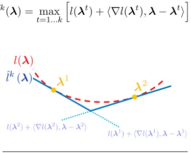
As shown in Figure 2, we can construct a cutting plane approximation of the loss function by taking the pointwise maximum of multiple cuts. In what follows, we denote the cutting plane approximation of the loss function built using kcuts as:
ˆlk(λ) = max t=1...k
h
l(λt) +h∇l(λt),λ−λtii.
l( )
1
2
Figure 2: A convex loss functionl(λ) and its cutting plane approximation ˆl2(λ).
On iterationk,CPAsolves a surrogate mixed-integer program (MIP) that minimizes the cutting plane approximation ˆlk, namely
Algorithm 1 Cutting Plane Algorithm (CPA) Input
(xi, yi)ni=1 training data
L coefficient set
C0 `0 penalty parameter
εstop∈[0,1] maximum optimality gap of acceptable solution
Initialize
k←0 iteration counter
ˆ
l0(λ)← {0} cutting plane approximation
(Vmin, Vmax)←(0,∞) bounds on the optimal value of
RiskSlimMINLP
ε← ∞ optimality gap
1: whileε > εstop do
2: (Lk,λk)←provably optimal solution to
RiskSlimMIP(ˆlk) 3: compute cut parametersl(λk) and∇l(λk)
4: ˆlk+1(λ)←max{ˆlk(λ), l(λk) +h∇l(λk),λ−λki}
update approximate loss functionˆlk 5: Vmin←Lk+C0
λk
0 optimal value of RiskSlimMIPis lower bound
6: if V(λk)< Vmax then
7: Vmax←V(λk) update upper bound
8: λbest←λk
update incumbent
9: end if
10: ε←1−Vmin/Vmax 11: k←k+ 1
12: end while
Output: λbest ε-optimal solution to
RiskSlimMINLP
RiskSlimMIP(ˆlk) is a surrogate problem forRiskSlimMINLP that minimizes a cutting
plane approximation ˆlk of the loss functionl:
min
L,λ L+C0kλk0 s.t. L≥ˆlk(λ)
λ∈ L.
(2)
to check for convergence. Here, the upper bound is set as the objective value of the best solution across all iterations:
Vmax= min t=1...k
h
l(λt) +C0kλtk0
i
.
The lower bound is set as the optimal value of the surrogate problem at the current iteration:
Vmin= ˆlk(λk) +C0kλkk0.
CPA converges to an optimal solution of RiskSlimMINLPin a finite number of
itera-tions (see e.g., Kelley, 1960, for a proof). In particular, the cutting plane approximation of a convex loss function improves monotonically with each cut:
ˆ
lk(λ)≤ˆlk+m(λ)≤l(λ) for all λ∈ Land k, m∈N.
Since the cuts added at each iteration are not redundant, the lower bound improves mono-tonically with each iteration. Once the optimality gap ε is less than a stopping threshold εstop,CPAterminates and returns anε-optimal solutionλbest to
RiskSlimMINLP.
Key Benefits of Cutting Plane Algorithms CPAhas three important properties that motivate why we want to use a cutting plane algorithm to solve the risk score problem:
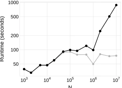
(i) Scalability in the Sample Size: Cutting plane algorithms use the training data only when computing cut parameters, and not while solving RiskSlimMIP. Since the
pa-rameters in (3) can be computed using elementary matrix-vector operations in O(nd) time at each iteration, running time scales linearly innfor fixed d(see Figure 3).
(ii) Control over Data-related Computation: Cutting plane algorithms compute cut pa-rameters in a single isolated step (e.g., Step 3 in Algorithm 1). Users can reduce data-related computation by customizing their implementation to compute these cut parameters efficiently (e.g., via distributed computing, or techniques that exploit struc-tural properties of a specific model class as in Section E.2).
(iii) Ability to use a MIP Solver: Cutting plane algorithms have a special benefit in our setting since the surrogate problem can be solved with a MIP solver (rather than a MINLP solver). MIP solvers provide a fast implementation of branch-and-bound search and other features to speed up the search process (e.g., built-in heuristics, preprocessing and cut generation procedures, lazy evaluation of cut constraints, and control callbacks that let us customize the search with specialized techniques). As we show in Figure 6, using a MIP solver can substantially improve our ability to solve RiskSlimMINLP,
despite the fact that one may have to solve multiple MIPs.
● ●
● ● ●
● ●
● ●
● ●
● ●
● ●
● ● ●
● ● ● ●
● ●
● ●
50 100 200 500 1000
103 104 105 106 107
N
Runtime (seconds)
Figure 3: Runtime ofCPAon synthetic datasets withd= 10 andn∈[103,107] (see Appendix D for details). Asnincreases, the runtime for the solver (grey) remains roughly constant. The total runtime (black) scales at O(n), which reflects the scalability of matrix-vector operations used to compute cut parameters.
is non-convex. In these settings, cutting plane algorithms will typicallystall as they even-tually reach an iteration where the surrogate problem cannot be solved to optimality within a fixed time limit.
In Figure 4, we illustrate the stalling behavior of CPAon a difficult instance of RiskSlim-MINLP for a synthetic dataset where d = 20 (see also Figure 6). As shown, the first
iterations terminate quickly as the surrogate problemRiskSlimMIP contains a trivial
ap-proximation of the loss. Since the surrogate becomes increasingly difficult to optimize with each iteration, however, the time to solve RiskSlimMIP increases exponentially, leading
CPAto stall at iterationk= 86. In this case, the solution returned byCPAafter 6 hours has a large optimality gap and a highly suboptimal loss. This is unsurprising, as the solution was obtained by optimizing a low-fidelity approximation of the loss (i.e., an 85-cut approxi-mation of a 20-dimensional function). Since the value of the loss is tied to the performance of the model (see Section 5), the solution corresponds to a risk score with poor performance.
0.01 0.1 1 10 100 1000 10000
10 20 50 100 200 500
Cuts Added
Seconds/Cut
0% 20% 40% 60% 80% 100%
10 20 50 100 200 500
Cuts Added
Optimality Gap
Figure 4: Performance profile of CPAonRiskSlimMINLPfor a synthetic dataset withn = 50,000 and
d = 20 (see Appendix D for details). We plot the time per iteration (left, in log-scale) and optimality gap (right) for each iteration over 6 hours. CPA stalls on iteration 86, at which point the time to solve
There is no simple fix to prevent standard cutting plane algorithms such as CPA from stalling on non-convex problems. This is because they need a globally optimal solution to a surrogate optimization problem at each iteration to compute a valid lower bound. In non-convex risk minimization problems, this requires finding the optimal solution of a non-convex surrogate problem, and certifying that there does not exist a better solution to the surrogate problem. If, for example, CPA only solved the surrogate until it found a feasible solution with a non-zero optimality gap, then it could produce a cutting plane that discards the true optimal solution. In this case, the lower bound computed in Step 5 would exceed the true optimal value, leading the algorithm to terminate prematurely and return a suboptimal solution with invalid bounds.
3.2. The Lattice Cutting Plane Algorithm
To avoid stalling in non-convex settings, we solve the risk score problem using the lattice cutting plane algorithm (LCPA) shown in Algorithm 2. LCPAhas the same benefits as other cutting plane algorithms for the risk score problem, such as scalability in the sample size, control over data-related computation, and the ability to use a MIP solver. As shown in Figure 5, however, LCPA does not stall. This is because it can add cuts and compute a lower bound without having to optimize a non-convex surrogate.
0.01 0.1 1 10 100 1000 10000
10 100 1000 10000
Cuts Added
Seconds/Cut
0% 20% 40% 60% 80% 100%
10 100 1000 10000
Cuts Added
Optimality Gap
Figure 5: Performance profile ofLCPA(red) andCPA(black) on theRiskSlimMINLPinstance in Figure 4. UnlikeCPA,LCPAdoes not stall. LCPArecovers a high-quality risk score (i.e., whose objective value is ≤10% of the optimal value) in 9 minutes after adding 4,655 cuts. The remaining time is used to reduce the optimality gap.
LCPA recovers the optimal solution to RiskSlimMINLPvia branch-and-bound (B&B)
search. The search process recursively splits the feasible region of RiskSlimMINLP,
Algorithm 2 Lattice Cutting Plane Algorithm (LCPA)
Input
(xi, yi)ni=1 training data
L coefficient set
C0 `0penalty parameter
εstop∈[0,1] optimality gap of acceptable solution
RemoveNode procedure to remove node from a node set (provided by MIP solver)
SplitRegion procedure to split region into disjoint subsets (provided by MIP solver)
RiskSlimLP(ˆl,R) LP relaxation ofRiskSlimMIP(ˆl) over the regionR ⊆conv (L) (see Definition 2) Initialize
k←0 number of cuts
ˆ
lk(λ)← {0} cutting plane approximation
(Vmin, Vmax)←(0,∞) bounds on the optimal value ofRiskSlimMINLP
R0←conv (L) initial region is convex hull of coefficient set
v0←0 lower bound of the objective value of the surrogate LP atR0
N ← {(R0, v0)} node set
ε← ∞ optimality gap
1: while ε > εstopdo
2: (Rt, vt)←RemoveNode(N) tis index of removed node
3: solveRiskSlimLP(ˆlk,Rt)
4: λt←coefficients from optimal solution toRiskSlimLP(ˆlk,Rt ) 5: Vt←optimal value ofRiskSlimLP(ˆlk,Rt
) 6: if optimal solution is integer feasiblethen 7: compute cut parametersl(λt) and∇l(λt)
8: ˆlk+1(λ)←max{ˆlk(λ), l(λt) +h∇l(λk),λ−λti} update approximate loss functionˆlk
9: if Vt< Vmax then
10: Vmax←Vt update lower bound
11: λbest←λt update best solution
12: N ← N \ {(Rs
, vs)|vs≥Vmax} prune suboptimal nodes
13: end if
14: k←k+ 1
15: else if optimal solution is not integer feasiblethen
16: (R0
,R00
)←SplitRegion(Rt
,λt) R0,R00are disjoint subsets ofRt
17: N ← N ∪ {(R0,Vt),(R00, Vt)} Vtis lower bound of RiskSlimLPfor child regionsR0,R00 18: end if
19: Vmin←min
s=1...|N |vs Vminis smallest lower bound among nodes inN
20: ε←1−Vmin/Vmax update optimality gap
21: end while
Output: λbest ε-optimal solution to
Definition 2 (RiskSlimLP)
Given a bounded convex region R ⊆conv (L), trade-off parameter C0>0, cutting plane
approximationˆlk:
Rd+1→R+ with cut parameters{l(λt),∇l(λt)}kt=1, and boundsVmin,
Vmax, Lmin, Lmax, Rmin, Rmax, the surrogate optimization problem
RiskSlimLP(ˆlk,R)
can be formulated as the linear program:
min
L,λ,α V
s.t. V = L+C0R objective value
R =
d
X
j=1
αj relaxed`0-norm
L ≥ l(λt) +h∇l(λt),λ−λti t= 1,...,k
cut constraints
λj ≤ Λmaxj αj j= 1,...,d `0-indicator constraints
λj ≥ −Λminj αj j= 1,...,d `0-indicator constraints
λ ∈ R feasible region
V ∈ [Vmin, Vmax] objective bounds
L ∈ [Lmin, Lmax] loss bounds
R ∈ [Rmin, Rmax] relaxed`0-bounds
αj ∈ [0,1] j= 1,...,d relaxed`0-indicators
Branch-and-Bound Search In Algorithm 2, we represent the state of the B&B search process using a B&B tree. We refer to each leaf of the tree as a node, and denote the set of all nodes as N. Each node (Rt, vt) ∈ N consists of: aregion of the convex hull of the coefficient setRt⊆conv (L); and a lower bound on the objective value of the surrogate LP over this regionvt.
Each iteration of LCPAremoves a node from the node set (Rt, vt)∈ N, then solves the surrogate LP for the corresponding region, that is,RiskSlimLP(ˆlk,Rt). Subsequent steps
of the algorithm are determined by the solution status of the surrogate LP:
• IfRiskSlimLP(ˆlk,Rt) has an integer solution,LCPAupdates the cutting plane
approxi-mation ˆlk with a new cut atλt in Step 8.
• If RiskSlimLP(ˆlk,Rt) has a real-valued solution, LCPA adds two child nodes (R0, vt)
and (R00, vt) to the node setN in Step 17. The child nodes are produced by applying a splitting rule, which splitsRtinto disjoint regions R0 andR00. The lower bound for each
child node is set as the optimal value of the surrogate LPvt.
• IfRiskSlimLP(ˆlk,Rt) is infeasible, thenLCPA discards the node from the node set.
The B&B search is governed by two procedures that are implemented in a MIP solver:
• RemoveNode, which removes a node (Rt, vt) from the node set N (e.g., the node with
the smallest lower boundvt).
• SplitRegion, which splits Rt into disjoint subsets ofRt (e.g., split on a fractional
compo-nent of λt, which returns R0 = {λ ∈ Rt|λt
j ≥ dλtje} and R
00 = {λ ∈ Rt|λt
LCPA evaluates the optimality of solutions to the risk score problem by using bounds on the objective value of RiskSlimMINLP. The upper boundVmax is set as the objective
value of the best integer feasible solution in Step 10. The lower bound Vmin is set as the
smallest objective value among all nodes in Step 19. The value of Vmin can be viewed as
a lower bound on the objective value of the surrogate LP over theremaining search region
S
tRt(i.e.,Vminis a lower bound on the objective value ofRiskSlimLP(ˆlk,
S
tRt)). Thus, Vmin will increase when we reduce the remaining search region or add cuts.
Each iteration of LCPAreduces the remaining search region by either finding an integer feasible solution, identifying an infeasible region, or splitting a region into disjoint subsets. Thus, Vmin increases monotonically as the search region becomes smaller, and cuts are
added at integer feasible solutions. Likewise, Vmax decreases monotonically as it is set as
the objective value of the best integer feasible solution. Since there are a finite number of nodes, even in the worst-case,LCPAterminates after a finite number of iterations, returning an optimal solution to the risk score problem.
Remark 3 (Worst-Case Data-Related Computation for LCPA) Given any training dataset (xi, yi)n
i=1, any trade-off parameter C0 > 0, and any finite
coefficient setL ⊂Zd+1,LCPAreturns an optimal solution to the risk score problem after
computing at most |L| cutting planes, and processing at most 2|L|−1 nodes.
Implementation with a MIP Solver with Lazy Cut Evaluation LCPA can easily be implemented using a MIP solver (e.g., CPLEX, Gurobi, GLPK) with control callbacks. In this approach, the solver handles the B&B related steps of Algorithm 2, and one needs only to write a few lines of code to update the cutting plane approximation when the algorithm finds an integer feasible solution. In a basic implementation, the solver would call the control callback when it finds an integer feasible solution (i.e., Step 6). The code would retrieve the integer feasible solution, compute the cut parameters, and add a cut to the surrogate LP, handing control back to the solver at Step 9.
A key benefit of using a MIP solver is the ability to add cuts as lazy constraints. In practice, if we were to add cuts as generic constraints to the surrogate LP, the time to solve the surrogate LP would increase with each cut, which would progressively slow down LCPA. When we add cuts as lazy constraints, the solver branches using a surrogate LP that contains a subset of relevant cuts, and only evaluates the complete set of cuts when LCPAfinds an integer feasible solution. In this case,LCPAstill returns the optimal solution. However, computation is significantly reduced as the surrogate LP is much faster to solve for the vast majority of cases where it is infeasible or yields a real-valued solution. From a design perspective, lazy cut evaluation reduces the marginal computational cost of adding cuts, which allows us to add cuts liberally (i.e., without having to worry about slowing downLCPAby adding too many cuts).
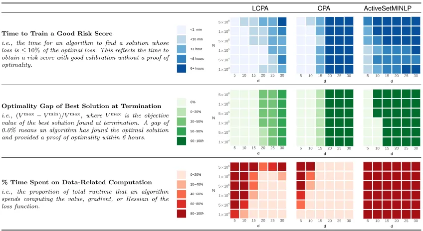
3.3. Performance Comparison with MINLP Algorithms
In Figure 6, we show the performance of algorithms on difficult instances of the risk score problem for synthetic datasets with d dimensions and n samples (see Appendix D for details). We consider the following performance metrics: (i) the time to find a near-optimal solution; (ii) the near-optimality gap of the best solution at termination; and (iii) the proportion of time spent on data-related computation. Since all three MINLP algorithms behave similarly, we only show the best one in Figure 6 (i.e., ActiveSetMINLP), and include results for the others in Appendix D.3.
As shown, LCPA finds an optimal or near-optimal solution for almost all instances of the risk score problem, and pairs the solution with a small optimality gap. CPA performs similarly to LCPA on low-dimensional instances. On instances with d≥15, however, CPA stalls after a few iterations and returns a highly suboptimal solution (i.e., a risk score with poor performance). In comparison, the MINLP algorithms can only handle instances with small n or d. On larger instances, the solver is slowed down by operations that involve data-related computation, fails to converge within the 6-hour time limit and fails to recover a high-quality solution. Seeing how MINLP solvers are designed to solve a diverse set of optimization problems, we do not believe that they can identify and exploit the structure of the risk score problem in the same way as a cutting plane algorithm.
LCPA CPA ActiveSetMINLP
Time to Train a Good Risk Score
i.e., the time for an algorithm to find a solution whose loss is≤10%of the optimal loss. This reflects the time to obtain a risk score with good calibration without a proof of optimality.
<1 min
<10 min
<1 hour
<6 hours
6+ hours 1×10⁴
5×10⁴
1×10⁵
5×10⁵
1×10⁶
5×10⁶
5 10 15 20 25 30 d N
1×10⁴
5×10⁴
1×10⁵
5×10⁵
1×10⁶
5×10⁶
5 10 15 20 25 30 d N 1×10⁴ 5×10⁴ 1×10⁵ 5×10⁵ 1×10⁶ 5×10⁶
5 10 15 20 25 30 d N
Optimality Gap of Best Solution at Termination i.e.,(Vmax−Vmin)/Vmax, whereVmaxis the objective value of the best solution found at termination. A gap of 0.0% means an algorithm has found the optimal solution and provided a proof of optimality within 6 hours.
0%
0−20%
20−50%
50−90%
90−100% 1×10⁴
5×10⁴
1×10⁵
5×10⁵
1×10⁶
5×10⁶
5 10 15 20 25 30 d N
1×10⁴
5×10⁴
1×10⁵
5×10⁵
1×10⁶
5×10⁶
5 10 15 20 25 30 d N 1×10⁴ 5×10⁴ 1×10⁵ 5×10⁵ 1×10⁶ 5×10⁶
5 10 15 20 25 30 d N
% Time Spent on Data-Related Computation i.e., the proportion of total runtime that an algorithm spends computing the value, gradient, or Hessian of the loss function.
0−20%
20−40%
40−60%
60−80%
80−100% 1×10⁴
5×10⁴
1×10⁵
5×10⁵
1×10⁶
5×10⁶
5 10 15 20 25 30 d N
1×10⁴
5×10⁴
1×10⁵
5×10⁵
1×10⁶
5×10⁶
5 10 15 20 25 30
d N 1×10⁴ 5×10⁴ 1×10⁵ 5×10⁵ 1×10⁶ 5×10⁶
5 10 15 20 25 30
d N
Figure 6: Performance of LCPA,CPA, and a commercial MINLP solver on difficult instances of
RiskSlim-MINLPfor synthetic datasets withddimensions andnsamples (see Appendix D for details).ActiveSetMINLP
fails to produce good risk scores on instances with largenordas it struggles with data-related computation.
4. Algorithmic Improvements
In this section, we describe specialized techniques to improve the performance of the lattice cutting plane algorithm (LCPA) on the risk score problem. They include:
• Polishing Heuristic. We present a technique called discrete coordinate descent (DCD;
Section 4.1), which we use to polish integer solutions found byLCPA(solutions satisfying the condition in Step 6). DCDaims to improve the objective value of all integer solutions, which produces stronger upper bounds over the course of LCPA, and reduces the time to recover a good risk score.
• Rounding Heuristic. We present a rounding technique called SequentialRounding
(Sec-tion 4.2) to generate integer solu(Sec-tions. We use SequentialRounding to round real-valued solutions of the surrogate LP (which are solutions that satisfy the condition in Step 15) and then polish the rounded solution with DCD. Rounded solutions may improve the best solution found by LCPA, producing stronger upper bounds and reducing the time to recover a good risk score.
• Bound Tightening Procedure. We design a fast procedure to strengthen bounds on the
optimal values of the objective, loss, and number of non-zero coefficients called ChainedUp-dates(Section 4.3). We callChainedUpdateswhenever the solver updates the upper bound in Step 10 or the lower bound in Step 19. ChainedUpdates improves the lower bound, and reduces the optimality gap of the final risk score.
We present additional techniques to improveLCPAin Appendix E such as an initializa-tion procedure and techniques to reduce data-related computainitializa-tion.
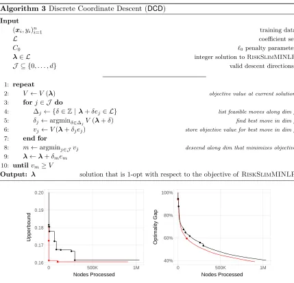
4.1. Discrete Coordinate Descent
Discrete coordinate descent (DCD) is a technique to polish an integer solution (Algorithm 3). It takes as input an integer solutionλ= [λ0, . . . , λd]> ∈ L and iteratively changes a single coordinate j to attain an integer solution with a better objective value. The coordinate at each iteration is set to minimize the objective value, i.e., j∈argminj0V λ+δj0ej0.
DCD terminates once it can no longer strictly improve the objective value along any coordinate. This eliminates the potential of cycling, and thereby guarantees that the proce-dure will terminate in a finite number of iterations. The polished solution returned byDCD satisfies a type of local optimality guarantee for discrete optimization problems. Formally, it is1-opt with respect to the objective value, meaning that one cannot improve the objective value by changing any single coefficient (see e.g., Park and Boyd, 2018, for a technique to find a 1-opt point for a different optimization problem).
In practice, the most expensive computation in DCDis finding a step-sizeδj ∈∆j that minimizes the objective along coordinate j (Step 5 of Algorithm 3). We can significantly reduce this computation by using golden section search. This approach requiresndlog2|Lj| flops per iteration compared tond|Lj|flops per iteration required by a brute force approach (i.e., which evaluates the loss for all λj ∈ Lj).
Algorithm 3 Discrete Coordinate Descent (DCD) Input
(xi, yi)ni=1 training data
L coefficient set
C0 `0 penalty parameter
λ∈ L integer solution toRiskSlimMINLP
J ⊆ {0, . . . , d} valid descent directions
1: repeat
2: V ←V(λ) objective value at current solution
3: forj∈ J do
4: ∆j ← {δ∈Z|λ+δej ∈ L} list feasible moves along dimj
5: δj ←argminδ∈∆jV (λ+δ) find best move in dimj
6: vj←V(λ+δjej) store objective value for best move in dimj
7: end for
8: m←argminj∈Jvj descend along dim that minimizes objective
9: λ←λ+δmem
10: untilvm≥V
Output: λ solution that is 1-opt with respect to the objective ofRiskSlimMINLP
● ●
● ● ● ● ●● ●
●
● ● ●
● 0.16
0.17 0.18 0.19 0.20
0 500K 1M
Nodes Processed
Upperbound
● ● ●
● ● ● ●
● ●
● ●
●
● ●
40% 60% 80% 100%
0 500K 1M
Nodes Processed
Optimality Gap
Figure 7: Performance profile of LCPA in a basic implementation (black) and withDCD (red). We use
DCDto polish every integer solution found by the MIP solver whose objective value is within 10% of the current upper bound. We plot the number of total nodes processed of LCPA(x-axis) against the upper bound (y-axis; left) and the optimality gap (y-axis; right). We mark iterations where LCPA updates the incumbent solution. Results reflect performance onRiskSlimMINLPfor a synthetic dataset withd= 30 andn= 50,000 (see Appendix D for details).
4.2. Sequential Rounding
SequentialRounding (Algorithm 4) is a rounding heuristic to generate integer solutions for the risk score problem. In comparison to na¨ıve rounding, which returns the closest rounding from a set of 2d+1possible roundings,SequentialRoundingreturns a rounding that iteratively
finds a local optimizer of the risk score problem.
Given a real-valued solutionλreal ∈conv (L), the procedure iteratively rounds one
com-ponent (up or down) in a way that reduces the objective of RiskSlimMINLP. On iteration
Algorithm 4 SequentialRounding Input
(xi, yi)ni=1 training data
L coefficient set
C0 `0 penalty parameter
λ∈conv (L) non-integer infeasible solution fromRiskSlimLP 1: Jreal← {j :λ
j6=dλjc} index set of non-integer coefficients
2: repeat
3: λj,up←(λ1, . . . ,dλ
je, . . . , λd) for allj∈ Jreal
4: λj,down←(λ1, . . . ,bλ
jc, . . . , λd) for all j∈ Jreal
5: vup←min
j∈JrealV(λj,up) 6: vdown←min
j∈JrealV(λj,down) 7: if vup< vdown then
8: k←argminj∈JrealV(λj,up) andλk ← dλke
9: else
10: k←argminj∈JrealV(λj,down) andλk ← bλkc
11: end if
12: Jreal← Jreal\ {k} 13: untilJreal=∅
Output: λ∈ L integer solution
d+ 1−k components to dλreal
j e or bλrealj c. To this end, it computes the objective of all feasible (component, direction)-pairs and chooses the best one. Formally, the minimization on iterationkrequires 2·(d+ 1−k) evaluations of the loss function. Thus, given that there ared+ 1 iterations,SequentialRounding terminates after 2·Pd
k=1k=d(d+ 1) evaluations
of the loss function.
In Figure 8, we show the impact of using SequentialRounding in LCPA. Here, we ap-ply SequentialRoundingto the non-integer solution of RiskSlimLPwhen the lower bound
changes (i.e., just after Step 3 of Algorithm 2), then polish the rounded solution usingDCD. As shown, this strategy can reduce the time required for LCPA to find a high-quality risk score, and attain a lower optimality gap.
4.3. Chained Updates
We describe a fast bound tightening technique called ChainedUpdates(Algorithm 5). This technique iteratively bounds the optimal values of the objective, loss, and`0-norm by
iter-atively setting the values ofVmin,Vmax,Lmin,Lmax, and Rmax in
RiskSlimLP. Bounding
these quantities over the course of B&B restricts the search region without discarding the optimal solution, thereby improving the lower bound and reducing the optimality gap.
Initial Bounds on Objective Terms We initializeChainedUpdateswith values ofVmin,
Vmax,Lmin,Lmax, andRmax that can be computed using only the training data (x
i, yi)ni=1
and the coefficient setL. We start with Proposition 4, which provides initial values forLmin
● ● ●
● ● ● ● ●
● ●
● ●
●
● ● ●● ● ●● ●
●
● ● ●
● 0.16
0.17 0.18 0.19 0.20
0 500K 1M
Nodes Processed
Upperbound
● ● ● ●
● ● ●
● ● ● ● ● ● ● ●
● ● ● ●
● ●
● ●
●
● ●
40% 60% 80% 100%
0 500K 1M
Nodes Processed
Optimality Gap
Figure 8: Performance profile ofLCPAin a basic implementation (black) and withSequentialRoundingand
DCD polishing (red). We call SequentialRounding to round non-integer solutions to RiskSlimLP in Step 15, and then polish the integer solution withDCD. We plot large points to show when LCPAupdates the incumbent solution. Results reflect performance onRiskSlimMINLPfor a synthetic dataset withd= 30 andn= 50,000 (see Appendix D for details). Here,SequentialRoundingand DCDreduce the upper bound and optimality gap of LCPAcompared to a basic implementation.
Proposition 4 (Bounds on Logistic Loss over a Bounded Coefficient Set)
Given a training dataset (xi, yi)ni=1 where xi ∈ Rd and yi ∈ {±1} for i = 1, . . . , n, consider the normalized logistic loss of a linear classifier with coefficients λ:
l(λ) = 1 n
n
X
i=1
log(1 + exp(−hλ, yixii)).
If the coefficients belong to a bounded setL, then the value of the normalized logistic loss must obeyl(λ)∈[Lmin, Lmax] for allλ∈ L,where:
Lmin = 1
n
X
i:yi=+1
log (1 + exp(−smax
i )) + 1 n
X
i:yi=−1
log (1 + exp(smin
i )),
Lmax= 1 n
X
i:yi=+1
log (1 + exp(−smini )) + 1 n
X
i:yi=−1
log (1 + exp(smaxi )), smini = min
λ∈Lhλ,xiifori= 1, . . . , n,
smaxi = max
λ∈Lhλ,xii fori= 1, . . . , n.
The value of Lmin in Proposition 4 represents the “best-case” loss in a separable setting
where we assign each positive example its maximal scoresmax
i , and each negative example its minimal scoresmin
i . Conversely,Lmax represents the “worst-case” loss when we assign each positive example its minimal scoresmin
i and each negative example its maximal scoresmaxi . We initialize the bounds on the number of non-zero coefficientsR to∈ {0, . . . , d}, trivially. In some cases, these bounds may be stronger due to operational constraints (e.g., we can set R ∈ {0, . . . ,5} if models are required to use ≤5 features). Having initialized Lmin, Lmax,
RminandRmax, we set the bounds on the optimal objective value asVmin=Lmin+C 0Rmin
and Vmax=Lmax+C
Algorithm 5 ChainedUpdates Input
C0 `0 penalty parameter
Vmin, Vmax, Lmin,Lmax,Rmin, Rmax initial bounds onV(λ∗
),l(λ∗) andkλ∗k0
1: repeat
2: Vmin←max Vmin, Lmin+C0Rmin
update lower bound onV(λ∗)
3: Vmax←min (Vmax, Lmax+C0Rmax) update upper bound onV(λ∗) 4: Lmin←max Lmin, Vmin−C0Rmax
update lower bound onl(λ∗) 5: Lmax←min Lmax, Vmax−C0Rmin
update upper bound onl(λ∗) 6: Rmax←minRmax, jVmax−Lmin
C0 k
update upper bound onkλ∗k
0
7: untilthere are no more bound updates due to Steps 2 to 6.
Output: Vmin, Vmax, Lmin,Lmax, Rmin,Rmax
Dynamic Bounds on Objective Terms In Propositions 5 to 7, we present bounds that can use information from the solver inLCPAto strengthen the values ofLmin,Lmax,Rmax,
Vmin andVmax(see Appendix A for proofs).
Proposition 5 (Upper Bound on Optimal Number of Non-Zero Coefficients)
Given an upper bound on the optimal value Vmax ≥ V(λ∗), and a lower bound on the
optimal lossLmin≤l(λ∗), the optimal number of non-zero coefficients is at most
Rmax=
Vmax−Lmin
C0
.
Proposition 6 (Upper Bound on Optimal Loss)
Given an upper bound on the optimal value Vmax ≥ V(λ∗), and a lower bound on the
optimal number of non-zero coefficients Rmin ≤ kλ∗k
0, the optimal loss is at most
Lmax=Vmax−C0Rmin.
Proposition 7 (Lower Bound on Optimal Loss)
Given a lower bound on the optimal value Vmin ≤ V(λ∗), and an upper bound on the
optimal number of non-zero coefficients Rmax≥ kλ∗k
0, the optimal loss is at least
Lmin=Vmin−C0Rmax.
Implementation In Algorithm 5, we present a bound-tightening procedure that uses the results of Propositions 5 to 7 to strengthen the values ofVmin,Vmax,Lmin,Lmax, andRmax
inRiskSlimLP.
Propositions 5 to 7 impose dependencies between Vmin, Vmax, Lmin, Lmax, Rmin and
Rmax that may produce a complex “chain” of updates. As shown in Figure 9,
a case where we callChainedUpdatesafterLCPAimprovesVmin. Say the procedure updates
Lmin in Step 4. If ChainedUpdatesupdates Rmax in Step 6, then it will also update Vmax,
Lmin,Lmax, andVmin. However, if ChainedUpdatesdoes not update Rmax in Step 6, then
it will not updateVmax,Lmin,Lmax,Vmin and terminate.
Considering these dependencies, Algorithm 5 applies Propositions 5 to 7 until it can no longer improve Vmin, Vmax, Lmin, Lmax or Rmax. This ensures that ChainedUpdates will
return its strongest possible bounds regardless of the term that was first updated.
Vmax
Vmin
Rmax
Lmax
Lmin
Vmin
Lmin Vmax
Lmax
Lmin
Vmin
5
4 6
5
2
2
Figure 9: All possible “chains” of updates inChainedUpdates. Circles represent “source” terms that can be updated byLCPAto triggerChainedUpdates. The path from each source term shows all bounds that can be updated by the procedure. The number in each arrow references the update step in Algorithm 5.
In our implementation, we callChainedUpdateswheneverLCPAimprovesVmaxorVmin
(i.e., Step 10 or Step 19 of Algorithm 2). If ChainedUpdatesimproves any bounds, we pass this information back to the solver by updating the bounds on the auxiliary variables in the RiskSlimLP (Definition 2). As shown in Figure 10, this technique can considerably
improve the lower bound and optimality gap over the course of LCPA.
0.00 0.05 0.10
0 500K 1M
Nodes Processed
Lo
w
erbound
●●
●
●●
●●
●
●
●
●
●
40% 60% 80% 100%
0 500K 1M
Nodes Processed
Optimality Gap
5. Experiments
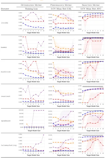
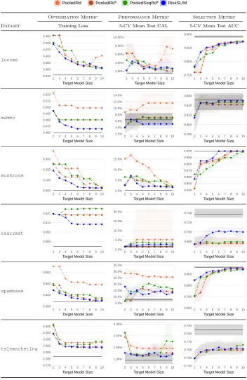
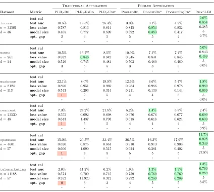
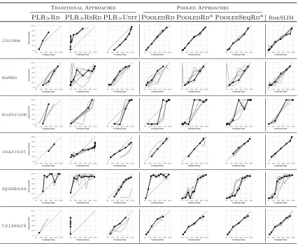
In this section, we compare the performance of methods to create risk scores. We have three goals: (i) to benchmark the performance and computation of our approach on real-world datasets; (ii) to highlight pitfalls of traditional approaches used in practice; and (iii) to present new approaches that address the pitfalls of traditional approaches.
5.1. Setup
We considered 6 publicly available datasets shown in Table 2. We chose these datasets to see how methods are affected by factors such as class imbalance, the number of features, and feature encoding. For each dataset, we fit risk scores using RiskSLIM and 6 baseline
methods that post-processed the coefficients of the best logistic regression model built using Lasso, Ridge or Elastic Net. We used each method to fit a risk score with small integer coefficients λj ∈ {−5, . . . ,5} that obeys the model size constraint kλk0 ≤ Rmax. We
benchmarked each method for target model sizes Rmax∈ {2, . . . ,10}.
Dataset n d Pr(yi= 1) Conditions foryi= 1 Reference
income 32,561 36 24.1% person in 1994 US census earns over $50,000 Kohavi (1996)
mammo 961 14 46.3% person has breast cancer Elter et al. (2007)
mushroom 8,124 113 48.2% mushroom is poisonous Schlimmer (1987)
rearrest 22,530 48 59.0% person is arrested after release from prison Zeng et al. (2017)
spambase 4,601 57 39.4% e-mail is spam Cranor and LaMacchia (1998)
telemarketing 41,188 57 11.3% person opens bank account after marketing call Moro et al. (2014)
Table 2: Datasets used in Section 5. All datasets are available on the UCI repository (Bache and Lichman, 2013), other thanrearrestwhich must be requested from ICPSR. We processed each dataset by dropping examples with missing values, and by binarizing categorical variables and some real-valued variables. We provide processed datasets and the code to processrearrestat http://github.com/ustunb/risk-slim.
RiskSLIM We formulated an instance of RiskSlimMINLP with the constraints: λ0 ∈
{−100, . . . ,100},λj ∈ {−5, . . . ,5}, andkλk0 ≤Rmax. We set the trade-off parameter to a
small value C0 = 10−6 to recover the sparsest model among equally accurate models (see
Appendix B). We solved each instance for at most 20 minutes on a 3.33 GHz CPU with 16 GB RAM using CPLEX 12.6.3 (ILOG, 2017).
Penalized Logistic Regression PLR is the best logistic regression model produced
over the full regularization path using a weighted combination of the `1 and `2 penalties
(i.e., the best model produced by Lasso, Ridge or Elastic Net). We trainPLRmodels using
theglmnetpackage of Friedman et al. (2010). The coefficients of each model are the solution to the optimization problem:
min
λ∈Rd+1
1 2n
n
X
i=1
log(1 + exp(−hλ, yixii)) +γ·
αkλk1+ (1−α)kλk22
where α ∈[0,1] is the elastic-net mixing parameter and γ ≥0 is a regularization penalty. We trained 1,100 PLR models by choosing 1,100 combinations of (α, γ): 11 values of
This free parameter grid produces 1,100PLR models that include models obtained by: (i)
Lasso (`1-penalty), which corresponds toPLR whenα= 1.0; (ii) Ridge (`2-penalty), which
corresponds toPLR when α = 0.0; (iii) standard logistic regression, which corresponds to PLR when α= 0.0 andγ is small.
Traditional Approaches While there is considerable variation in how risk scores are developed in practice, many researchers follow a two-step approach: (i) fit a sparse logistic regression model with real-valued coefficients; (ii) convert it into a risk score with integer coefficients. We consider three methods that adopt this approach. Each method first trains aPLR model (i.e., the one that maximizes the 5-CV AUC and obeys the model size
constraint), and then converts it into a risk score by applying a common rounding heuristic:
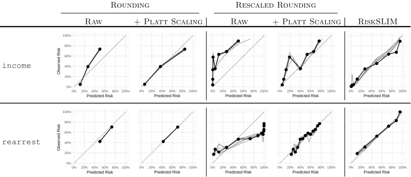
• PLRRd (Rounding): We round each coefficient to the nearest integer in {−5. . .5} by
setting λj ← dmin(max(λj,−5),5)c, and round the intercept asλ0 ← dλ0c.
• PLRUnit(Unit Weighting): We round each coefficient to±1 asλj ←sign(λj)1[λj 6= 0].
Unit weighting is a common heuristic in medicine and criminal justice (see e.g., Antman et al., 2000; Kessler et al., 2005; U.S. Department of Justice, 2005; Duwe and Kim, 2016), and sometimes called the Burgess method (as it was first proposed by Burgess, 1928).
• PLRRsRd (Rescaled Rounding) We first rescale coefficients so that the largest
coef-ficient is ±5, then round each coefficient to the nearest integer (i.e., λj → dγλjc where γ = 5/maxj|λj|). Rescaling is often used to avoid rounding small coefficients to zero, which happens when |λj|<0.5 (see e.g., Le Gall et al., 1993).
Pooled Approaches We also propose three new methods that use a pooling strategy and the loss-minimizing heuristics from Section 4. Each method generates a pool of PLR
models with real-valued coefficients, applies the same post-processing procedure to each model in the pool, then selects the best risk score among feasible risk scores. The methods include:
• PooledRd (Pooled PLR + Rounding): We fit a pool of 1,100 models using PLR. For
each model in the pool, we round each coefficient to the nearest integer in{−5, . . . ,5}by setting λj ← dmin(max(λj,−5),5)c, and round the intercept asλ0 ← dλ0c.
• PooledRd*(PooledPLR+ Rounding + Polishing): We fit a pool of 1,100 models using
PooledRd. For each model in the pool, we polish the rounded coefficients usingDCD.
• PooledSeqRd* (Pooled PLR + Sequential Rounding + Polishing): We fit a pool of
1,100 models using PLR. For each model in the pool, we round the coefficients using
SequentialRoundingand then polish the rounded coefficients using DCD.
To ensure that the polishing step in PooledRd*and PooledSeqRd* does not increase
the number of non-zero coefficients (which would violate the model size constraint), we run DCDonly on the set{j |λj 6= 0} (i.e., by fixing the set of zeros coefficients).
Performance Evaluation We evaluate the calibration of each risk score by plotting a reliability diagram, which shows how the predicted risk (x-axis) matches the observed risk (y-axis) for each distinct score (DeGroot and Fienberg, 1983). Theobserved risk at a score of sis defined as
¯ ps=
1
|{i:si=s}|
X
i:si=s