Scalable Computing: Practice and Experience
Volume 9, Number 2, pp. 95–100. http://www.scpe.org
ISSN 1895-1767 c
2008 SCPE
SIMULATION MODELS OF NATURAL DISASTERS AND SERVICE-BASED VISUALIZATION OF THEIR DATASETS IN THE MEDIGRID PROJECT∗
PETER SL´IˇZIK†AND LADISLAV HLUCH ´Y†
Abstract. Computational models of natural disasters are invaluable means of disaster reconstruction, crisis management, and disaster prevention. The Medigrid project addressed these issues by developing a framework of simulation models developed in previous projects. The paper describes the models incorporated into the project, together with the visualization service developed for presentation of models’ outputs.
Key words: scientific visualization, grid computing, Web services, map services
1. Introduction. This paper describes the Medigrid project, a European RTD project, objective of which was to develop a framework for multi-risk assessment of natural disasters and integrate models developed in the previous projects [1]. The paper is an extension of the paper [2] presented at PPAM 20071.
The text puts special emphasis on the models of disasters and on the visualization tools used in the project. The visualization service, which was the core of paper [2], was later extended with its three-dimensional version, which is also discussed here.
2. Simulation of Natural Disasters. Natural disasters have been addressed by many research projects. The ability to model a disaster on a computational system is invaluable. There are three main reasons which motivate the research and development of disaster models:
Reconstruction of past events. A comparison of simulated disasters with the actual event records helps reconstruct the most probable cause of the disaster (like the location of ignition points in case of fire) and evaluate the efficiency of disaster fighting activities.
Simulation of ongoing disasters. Simulation of ongoing events is a strong decision support tool for risk management teams. The models allow to forecast different scenarios of disaster propagation and help find best places for placement of barriers or identify locations that must be evacuated urgently.
Simulation of potential disasters. Fictitious disasters are simulated for two reasons: first, to assess the degree of damage that even the most unprobable events can cause and be prepared for them; and second, for educational and training purposes for mitigation teams.
3. The Medigrid Project. As stated before, the goal of the Medigrid project was to integrate simula-tion models of natural disasters developed in the previous projects and develop a unified framework for their management. Unfortunately, some of the models were interactive-only (i. e., incapable of being run in batch environment); some other were just not grid-aware. In order to be able to run in the Grid infrastructure, they had to be gridified. The task was made more difficult by different requirements of applications; as they had been developed unaware of one another, they were both sequential and parallel, and running both on Unix and Windows operating systems. The state-of-the-art Grid infrastructure (particularly the GridFTP service) sup-ported data exchange between Unix applications only; data communication with Windows-based applications had to be implemented from scratch.
3.1. Technology. The models provided by the members of the project consortium can be looked upon as a set of loosely coupled services [3]. In order to make them accessible from the standard Grid environment, each of the system components is exposed as a web service. The WSRF technology [4] was chosen as the basic implementation framework. This technology also helps glue the individual components together in a workflow-like manner.
Understandably, the big challenge of the Medigrid project was the dual Linux and Windows nature of the models; the reason being that the models were already developed by project partners or third parties
∗This work was supported by projects MEDIGRID EU 6FP RTD SustDev Project: Mediterranean Grid of Multi-Risk Data and
Models (2004–2006), GOCE-CT-2003-004044 (Call FP6-2003-Global-2, STREP) and VEGA No. 2/6103/6.
†Institute of Informatics, Slovak Academy of Sciences, D´ubravsk´a cesta 9, 845 07 Bratislava, Slovakia, {peter.slizik,
hluchy.ui}@savba.sk 1
PPAM 2007—Seventh International Conference on Parallel Processing and Applied Mathematics, September 9–12, 2007, Gda´nsk, Poland.
96 Peter Sl´ıˇzik and Ladislav Hluch´y
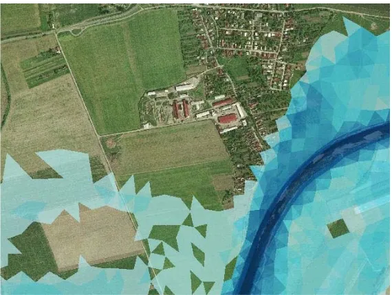
Fig. 3.1.Visualization of a flood simulation on the V´ah river, Slovakia. The water poured out of the river bed and endangers the village. The intensity of colour shows the depth of the water. The colour turns into black in the river bed.
respecting the local conventions. For the need to support both platforms, the Java implementation of the WSRF specification by the Globus Alliance had been chosen.
The Medigrid architecture consists of six core services: Data Management Servicefor platform-independent management of data sets,Data Transfer Servicefor the copying of data between cooperating services,Metadata Catalogue Service for publishing, discovery, and access to metadata for large-scale datasets,Job Management Service for automated platform-independent management of applications, and theGeovisualization service for drawing the simulation results to maps. An essential part of the system is the Distributed Data Repository, which is a decentralised storage for both, the input digital maps, and the outputs produced by the simulations. The whole system is accessible via a web portal. Application specific portlets allow users to invoke all services in application-specific manner. There are portlets for browsing input data, simulation results, their respective metadata, and also portlets for monitoring and house-keeping functions. The GridSpere portal [5] was chosen as the implementation platform for its support of portlet specification.
3.2. Models. The disaster simulation models incorporated into the Medigrid project include simulation of floods, landslides, forest fires, and soil erosion. All models were developed by the respective project members, except of the models used in the flood simulation application, which were developed by third-party institutions.
3.2.1. Flood Forecasting. The flood forecasting application consists of several simulation models (mete-orological, hydrological, and hydraulics). The models are connected into a cascade; outputs from one model are used as inputs for the next one. Meteorological models are used to forecast precipitation, which is used by the hydrological model to compute river discharge. That is used in turn in the final step for the actual computation of a possible flood by the hydraulics model. The output data generated by the models are then used to generate maps visualizing the simulation.
The flood prediction application supports two meteorological models, they can be used interchangeably. The first one,Aladin[6], is a mesoscale meteorological simulation model developed by Meteo France. Meteorological models solve the so-called “atmosphere equations” on a regular terrain grid. The global model (operated by Meteo France) computes forecasts for the whole Earth on a small-resolution grid, the global weather situation is then used to set the boundary condition for a locally-operated high-resolution model.
The other model, MM5[7], is a limited-area, terrain-following model designed to simulate and predict mesoscale and regional-scale atmospheric circulation. Since MM5 is a regional-area model too, it requires the initial conditions supplied by the global model.
sur-Simulation Models and Visualization in Medigrid 97
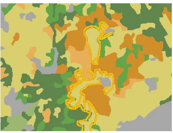
Fig. 3.2. Visualization of a forest fire simulation. The different background colours represent different types of vegetation (grass, shrubs, trees, etc.) The small circles show the progress of the fire. The spread of the fire corresponds with the areas of grass cover.
faces and in streams for extended periods of time. HSPF uses continuous rainfall and other meteorologic records to compute hydrographs. HSPF simulates many quantities, such as interception soil moisture, surface runoff, snowmelt, and evapotranspiratrion. Only a few values, most importantly river discharge, are interesting for the consecutive hydraulic model.
The river discharge computed by HSPF is fetched toDaveF, a hydraulic finite-element simulation model. The model works with limited irregular terrain mesh; a few values such as water depth, direction, and speed are computed for each mesh element in a given time step. The output of this model is treated as the input for the visualization module, which in turn draws DaveF’s simulated data into the map. The map shows the depth of water in the river bed and the adjacent areas, giving the crisis teams hints as to which regions need special attention (see Fig. 3.1).
3.2.2. Water Flow and Sediment Transport. Water flow and sediment transport in river basins were modelled by theSHETRAN model. The model provides the hydrological and sediment transport framework for the landslide model. It can be applied to a single basin, to parts of a basin and to groups of contiguous basins. The model depends on meteorological data such as precipitation and evapotranspiration and catchment property data such as topography, soil types, vegetation types, and sediment characteristics. Output includes flow rates, rates of ground surface erosion, sediment discharge rates, and debris flow rates. The model consists of three components: water flow component, sediment transport component, and landslide component.
The water flow component deals with surface water flow on the ground surface and in stream channels. The following processes are simulated: canopy interception of rainfall, evaporation and transpiration, infiltration to surface, and surface runoff.
The sediment transport component deals with soil erosion and multifraction transport on the ground sur-face and in stream channels. The simulated processes include erosion by raindrop, deposition and storage of sediments, erosion of river beds and banks, and deposition on river bed.
The landslide component simulates the erosion and sediment yield associated with shallow landslides. The simulated processes include landslide incidence, debris flow transport, direct sediment delivery to the channel system, and transport of sediment along the river system.
The simulation model identifies regions of the basin that are at risk from landslides and calculates the soil saturation conditions critical for triggering a landslide at a given location.
98 Peter Sl´ıˇzik and Ladislav Hluch´y
Fig. 4.1.Visualization of a forest fire in the Krompl’a region, Slovensk´y Raj National Park, Slovakia.
FireStation simulator implements a semi-empirical model for the rate of fire spread. The simulator works with the elliptical model. It is based on Huygens’ principle, which states that each point of the fireline becomes a new ignition point and starts a new local fire in the shape of an ellipse. The front line of the fire is represented by the envelope of all ellipses generated at each point.
Algosystemsimulator calculates the danger of occurence of a forest fire in a known geographical target area and simulates the propagation of such a fire, which is deemed to have started within this area.
Both systems work, in their particular way, with geographical data (terrain, slope, and fuel coverage data), meteorological data (wind speed and direction, temperature and relative humidity of air, rainfall), and the location of the point(s) of ignition as inputs.
Based upon the data, the FireStation software computes the evolution of the fire shape in time, the rate of the spread of fire, and fire intensity. The Algosystems software computes a map indicating the danger of fire occurence, and an abstract representation of a series of contours that indicate the projected state of a fire at the various points in the simulation period (see Fig. 3.2).
In addition to local-level prediction, the models also incorporate a fire danger rating system applicable at regional and national level. The rating system incorporates the Canadian Fire Weather Index, which is a set of indicators for the easiness of ignition and spread, the moisture content of loosely compacted for-est floor organic layers, and the moisture of deep and compacted floor organic layers. The Fire Weather Index is the final component of the system and gives a numerical rating of the potential frontal fire inten-sity.
The algorithms for calculating the danger indices work cumulatively. That means the value calculated for an index for a given day takes into account the value computed for the previous day. Over time, the indices become more accurate and more linked to the meteorological history of the target area.
4. Visualization. Historically, each of the supported models had its own means of data visualization. For instance, the results of the third-party DaveF flood simulation model were displayed by a system based on the GRASS GIS software [9]. Other models implemented their own visualization engines. For compatibility reasons, a decision was made to create a unified way of data visualization. The Geovisualization service accomplished this for 2D maps, the 3D visualization tool developed later has accomplished it for 3D virtual worlds.
Simulation Models and Visualization in Medigrid 99
The first, non-interactive part is responsible for preparing the simulation outputs for the rendering part. This part parses the input files, does the necessary conversions, prepares colour palettes, generates templates, etc.
The second, interactive part, provides the user interface. It consists of two components, a server-side component responsible for data rendering, and a client-side part.
The server-side component is based on Minnesota MapServer [10], an open-source, multi-platform framework for the development of spatially enabled web applications. Unlike full-featured GISes, which are capable of complex data analyses, map servers focus strongly on data rendering. Their outputs are designed for embedding into web pages. MapServer supports many vector and raster data formats through third-party OGR [11] and GDAL [12] libraries. MapServer is valued for the easiness of configuration, simple programming model, and excellent documentation.
The client is invoked by the user from the internet browser. The Medigrid portal provides a suitable map client for easy access to geographical data and simulation results.
4.2. The 3D Visualization Tools. The 3D visualization tool is a successor to the Geovisualization Service. Its task is to create VRML-based 3D worlds from the same input data that the Geovisualization Service uses.
The 3D tool works in three phases. Firstly, the input data are collected and fetched from the simulation application. In the next step, they are converted into a displayable form (virtual scenes). The last step is the display of virtual scenes on user’s device. The first phase runs in the Grid, the last one on the user’s computer. The second phase can be run in both environments, depending on the decision of the designer. Placing this phase into the Grid environment enables it to use vast Grid computational resources.
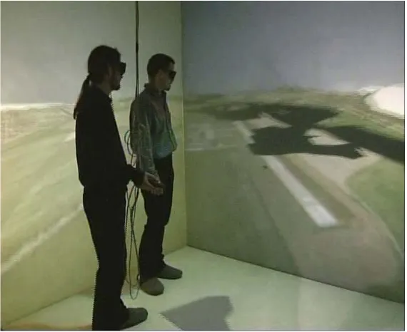
Using an appropriate plugin, the VRML virtual scenes can be displayed in a standard web browser (see Fig. 4.1). The scenes have already been successfully ported to a full-featured Virtual Reality device (see Fig. 5.1).
4.3. Input and Output Data. The data with which the service works differ according to the simulation being computed; however, they share some common core. Typically, each visualization uses a background image that serves as a reference to which other map elements are related. The outputs of simulations are rendered on this background; sometimes assissted with another reference mesh. The following four types of data are seen in virtually all visualization systems for geographical simulations:
Terrain texture. It is an image (usually an orthophotomap) used as a background for referencing other map elements.
Terrain model. Often referred to with acronyms DEM (Digital Elevation Model) and DTM (Digital Terrain Map). Used by the 3D visualization tool.
Reference structure. A mesh of polygons or a set of points that the simulation algorithm actually works with. Drawing this structure on the map may prove helpful for the end user.
Simulation results. The actual (numerical) results of simulations. They almost always represent time steps showing the development of the disaster in time.
The terrain model and terrain texture files use raster data formats. The Medigrid system directly supports ARC/INFO ASCIIGRID [13] [14] and GRASS ASCII [15] formats. Other formats are supported by the GDAL library [12] (used by MapServer). The reference structure and other auxiliary data are stored in vector formats. ESRI Shapefile [16], MapServer’s native format, is supported directly. Other vector formats are supported through the OGR library [11]. Imagery data are stored in general image formats such as JPEG, GIF, PNG, or TIFF.
5. Conclusions. The Medigrid project has succeeded in creating a framework for multi-risk assessment of natural disasters. The provided models were gridified (accomodated for the use in Grid infrastructure) and the interactive models were adapted for the use with the WSRF protocol. Together with the supporting infrastructure and the web portal, the project has created an easy-to-use virtual laboratory for running natural disaster simulations.
The Geovisualization Service has provided an unified means of visualization for the simulation models. Both, spatial and temporal progress of an event can be visualized. The service is scalable, e.i., it is able to display simulations consisting either of a few or a few hundreds of time steps.
100 Peter Sl´ıˇzik and Ladislav Hluch´y
Fig. 5.1. Visualization of a simulated flood on the V´ah river in the CAVE virtual reality device. Virtual Reality Center, Institute of Graphics and Parallel Processing, Johannes Kepler University Linz, Austria.
REFERENCES
[1] L. Hluch´y, O. Habala, G. Nguyen, B. ˇSimo, V. Tran, M. Bab´ık,Grid computing and knowledge management in EU RTD projects of IISAS, in Proceedings of 1st
International Workshop on Grid Computing for Complex Problems—GCCP 2005, VEDA, Bratislava, Slovakia, 2006, pp. 7–19, ISBN 80-969202-1-9.
[2] P. Sl´ıˇzik, L. Hluch´y,Geovisualisation Service for Grid-based Assessment of Natural Disasters, LNCS 4967, 2008, presented at PPAM 2007—Seventh International Conference on Parallel Processing and Applied Mathematics, September 9–12, 2007, Gda´nsk, Poland.—in print—
[3] B. ˇSimo, M. Ciglan, P. Sl´ıˇzik, M. Maliˇska, M. Dobruck´y, Mediterranean Grid of Multi-Risk Data and Models, in Proceedings of 1st
International Workshop on Grid Computing for Complex Problems—GCCP 2005, VEDA, Bratislava, Slovakia, 2006, pp. 129–134, ISBN 80-969202-1-9.
[4] Web Service Resource Framework, The Globus Alliance, http://www.globus.org/wsrf/ [5] GridSphere Portal Framework, http://www.gridsphere.org
[6] ALADIN Numerical Weather Prediction Project, Meteo France,http://www.cnrm.meteo.fr/aladin/ [7] MM5 Community Model, National Center for Atmosperic Research, Pennsylvania State University,
http://www.mmm.ucar.edu/mm5/
[8] Hydrological Simulation Program—Fortran (HSPF), Water Resources of United States, U.S. Geological Survey, http://water.usgs.gov/software/HSPF/
[9] Geographic Resources Analysis Support System GRASS, http://grass.itc.it [10] Minnesota MapServer, http://mapserver.gis.umn.edu/
[11] OGR Simple Feature Library, http://www.gdal.org/ogr/
[12] GDAL—Geospatial Data Abstraction Library, http://www.gdal.org/
[13] ARC/INFO ASCIIGRID file format description,http://www.climatesource.com/format/arc asciigrid.html [14] ESRI ARC/INFO ASCII raster file format description (GRASS manual),
http://grass.itc.it/grass63/manuals/html63 user/r.in.arc.html
[15] GRASS ASCII raster file format description,http://grass.itc.it/grass63/manuals/html63 user/r.in.ascii.html [16] ESRI Shapefile Technical Description, an ESRI white paper, Environmental Systems Research Institute, Inc., 1998,
http://www.esri.com/library/whitepapers/pdfs/shapefile.pdf
Edited by: Dana Petcu, Marcin Paprzycki
Received: May 4, 2008