Volume 10, Number 4, pp. 347–361. http://www.scpe.org c 2009 SCPE
CONDITIONING AND HYBRID MESH SELECTION ALGORITHMS FOR TWO-POINT BOUNDARY VALUE PROBLEMS∗
JEFF R. CASH†ANDFRANCESCA MAZZIA‡
Abstract. Boundary value problems for ordinary differential equations (BVODES) occur in a great many practical situations and they are generally much harder to solve than initial value problems. Traditionally codes for BVODES did not take into account the conditioning of the problem and it was generally assumed that the problem being solved was well conditioned so that small local errors gave rise to correspondingly small global errors. Recently a new generation of codes which take account of conditioning has been developed. However most of these codes are based on a rather ad hoc approach with the need to choose several heuristics without any real guidance on how these choices can be made. In this paper we identify clearly which heuristics need to be chosen and we discuss different choices of monitor functions that are used in our codes. This has the important effect of unifying the various approaches that have recently been proposed. This in turn allows us, in the present paper, to introduce a new technique for computing the conditioning which is ideally suited to BVODES.
1. Introduction. The task of solving systems of nonlinear two-point boundary value problems numerically has, for a long time, received a great deal of attention. Boundary value problems for ordinary differential equations (BVODES) occur in a great many practical situations and they are generally much harder to solve than initial value problems. In particular the numerical solution of singular perturbation problems can be especially difficult because such equations can have solutions with very narrow regions of rapid variation typified by boundary layers, shocks and interior layers.
Traditionally codes for BVODES did not take into account the conditioning of the problem and it was generally assumed that the problem being solved was well conditioned so that small local errors gave rise to correspondingly small global errors. However, in an important paper by Shampine and Muir [28], the need to consider the conditioning of the problem being solved was clearly demonstrated by means of a numerical example and this brought into focus some important earlier work by Brugnano and Trigiante [5, 6] and by Mazzia and Trigiante [27] who derived codes with a monitor function depending on both conditioning and error. Subsequently a new generation of codes which take account of conditioning has been developed. However most of these codes are based on a rather ad hoc approach with the need to choose several heuristics without any real guidance on how these choices can be made. In this paper we identify clearly which heuristics need to be chosen and we discuss different choices of monitor functions that are used in our codes. This has the important effect of unifying the various approaches that have recently been proposed. This in turn allows us, in the present paper, to introduce a new technique for computing the conditioning parameters which is ideally suited to BVODES. Finally we describe some codes which implement these new ideas and we give some numerical results obtained from using these codes.
We will only consider in this paper singular perturbation boundary value problems, although the algorithms developed are designed for general first order boundary value problems. We will not be concerned in this paper with shooting methods but will instead confine our attention to so called finite difference or boundary value methods. However a lot has been done on estimating the conditioning of shooting methods and the interested reader is referred to [1, 20, 21, 19, 13].
In section 2 we give a review of the algorithms based on conditioning for singularly perturbed boundary value problems. In section 3 we present the conditioning parameters for the continuous problem and in section 4 the corresponding parameters for the discrete one. In section 5 we analyze the hybrid mesh selection strategies based on conditioning and the way they have been unified and updated. In section 6 we present the results of some numerical experiments to analyze the behavior of the codes with the new condition estimator.
2. Singular Perturbation Problems.
2.1. Second Order Scalar Problems. The first attempt to use conditioning in algorithms for the solu-tion of singularly perturbed BVODES was made in [24, 8] by Mazzia and Trigiante. The algorithm presented in [24, 8] was designed for the following general class of scalar linear problems:
∗Work developed within the project “Numerical methods and software for differential equations”
†Department of Mathematics, Imperial College, South Kensington, London SW7, England
‡Dipartimento di Matematica, Universit`a di Bari, Via Orabona 4, I-70125 Bari, Italy
ǫy′′+p(x)y′+q(x)y=f(x)
y(a) =ya, y(b) =yb, a≤x≤b,
(2.1)
whereǫis a positive parameter which is small compared withb−a,q(x) andf(x) are continuous functions and
p(x) is differentiable.
If we discretize (2.1) using simple three point finite difference formulae, the discrete problem is a tri-diagonal system of algebraic equations that can be solved to give an approximation to the solution of (2.1). In matrix form this system is
Ty =f (2.2)
wherey0, y1, . . . , yn is the numerical solution computed on the meshπ={x0, x1, . . . , xn},y= (y1, y2, . . . , yn)T and
T =
1 τ1
σ1 1 τ2
σ2 1 . ..
. .. ... τn−1
σn−1 1
. (2.3)
The matrix T depends onπ and the algorithm presented in [24, 8] uses sufficient conditions for the well conditioning of tridiagonal matrices derived in [3] to compute the mesh. This allows us to derive, for example, the conditions that a constant stepsize, h, should satisfy in order to have T well conditioned. In general we requireh≈O(√ǫ). However in the much more important case where we solve (2.1) using a variable meshsize the mesh must be choosen in order to have then×nsystem (2.2) such that n≪ 1ǫ.
In [24, 8] Mazzia and Trigiante, using only information related to the well conditioning of the tridiagonal matrixT, derive second order methods for the solution of (2.1) where the grid is chosen so that
1. The user requested accuracy is achieved.
2. The inverse coefficient matrix T−1 exists and its condition number is either independent of n (well conditioned) or grows asnorn2 (weakly well conditioned).
The way that these two conditions are satisfied is to choosehiin order to have (σi, τi) that satisfy the conditions for the (weakly) well-conditioning ofT. The algorithm simplifies considerably ifσi andτi have constant sign. We note that in a classical approach, where ǫ is not small, it would be normal to choose σi and τi so that the matrix T is diagonally dominant. However in this case h is of the order ǫ and n is of order 1
ǫ and this is unacceptable when ǫ is very small. An algorithm that chooses τi and σi so that 1) and 2) are satisfied is described in [8] and some numerical results presented for singular perturbation problems show the power of the method.
2.2. First Order Systems of Singular Perturbation Problems. Although the algorithm described in the previous section represented a major step forward in the solution of singular perturbation problems it has the disadvantage that it is only applicable for linear, scalar, second order systems, it is of low order and it is not very easy to apply for variable stepsizes. However the strategy of using conditioning in choosing the mesh size is an important one and in the following sections we will discuss how to deal with nonlinear systems of BVODES.
In what follows we will be concerned with the nonlinear system of singular perturbation problems
D(ǫ)y′(x) =f(x, y), a≤x≤b, g(y(a), y(b)) = 0, (2.4)
where D(ǫ) is a diagonal matrix whose elements depend linearly on ǫ. Usually D(ǫ) = diag(1, . . . ,1, ǫ), and
grid points are clustered in regions of rapid variation of the solution and relatively few grid points are placed in regions where the solution is smooth. Most codes attempt to control the error in the solution either by estimating the discrete error at the mesh points [7] or else by controlling a residual [28]. The important point to realise is that in both cases the codes attempt to control the local error on the assumption that the problem is well conditioned so that if the local error is small then the global error will also be small. However in the case where the problem is ill-conditioned a standard backward error analysis shows that it is possible for an accepted solution to have a small local error but to have an unacceptably large global error. There is the additional problem that if a monitor function ( [1], p. 363) takes no account of conditioning of a problem then the grid choosing algorithm may become very inefficient. This is manifested by a sort of cycling where points are added into the grid on conditioning considerations and are then removed in the next remeshing due to accuracy considerations. To illustrate these ideas we present a test problem which we solve by using the code TWPBVPC [11] both with the standard mesh selection strategy based on the estimation of the local error and with a mesh selection strategy which considers both conditioning and local error estimation. We note that to change from the code TWPBVPC, which takes account of conditioning, to TWPBVP, which uses a conventional mesh choosing strategy, we need to change just one input parameter of the code TWPBVPC.
Example 1. We examine the following problem [11] :
ǫy′′+xy′=−ǫπ2cos(πx)−πxsin(πx),
y(−1) =−2, y(1) = 0, (2.5)
whose exact solution is cos(πx) + erf(x/√2ǫ)/erf(1/√2ǫ), solved using the code TWPBVP when conditioning is not taken into account. The problem is rewritten as a first order system with two components (y, y′)T and the input parameters areǫ= 10−7andtol(y) = 10−8. This means that we are seeking an approximation to the solution with an error 0.5·10−8or less in theycomponent. The code gives a solution using a final mesh of 4192 points with a maximum error of 0.17·10−8. The mesh sizes used in the intermediate steps of the computation are: 16, 31, 61, 121, 241, 481, 530, 1059, 1108, 2215, 2242, 4483, 8965, 19912, 4192. It seems that the code finds the problem very difficult to solve and it needs 19912 mesh points to get some worthwhile information about the solution. This is mainly due to the fact that the mesh selection algorithm adds extra points in the wrong place. If we use the same code with the mesh selection based on conditioning, and we call this TWPBVPC, the solution is obtained using 368 mesh points with maximum error of 0.85·10−8. The meshes used are of sizes: 16, 31, 58, 85, 169, 368. The information given by the conditioning parameters allows the code to put the mesh points in the correct place and makes it considerably more efficient for the solution of this problem.
The first papers to consider this problem of estimating the conditioning constants in a serious way were by Brugnano and Trigiante [4, 5] and by Mazzia and Trigiante [27]. Their basic approach is to identify two con-stants which characterise the conditioning of the continuous problem. Having done this the monitor function used in the mesh choosing algorithm is based on the relative size of these two parameters as well as on a local error estimate. The basic aim of the algorithm described in [27] is to choose the mesh so that the discrete and continuous problems have conditioning parameters which have the same order of magnitude. Perhaps the first really powerful code that used a monitor function based on accuracy and conditioning was the code TOM [27]. Numerical results presented in [27] show the excellent performance of this code compared with the case where conditioning is not considered. Using ideas explained in [27] the two deferred correction codes TWPBVP and TWPBVPL were modified to include conditioning in their monitor function and the much improved perfor-mance of the modified codes TWPBVPC and TWPBVPLC can be seen from the results on the authors’ web page [11].
3. Conditioning parameters. To introduce the conditioning parameters which will be used in the mesh selection strategy of our codes, let us consider for simplicity the following linear boundary value problem:
dy
dx =A(x)y(x) +q(x), a≤x≤b, Bay(a) +Bby(b) =β, β∈R
m (3.1)
whose solution is given by
y(x) =Y(x)Q−1β+
Z b
a
HereY(x) is a fundamental solution,Q=BaY(a) +BbY(b) is non singular andG(x, t) is the Greens’ function. Using the∞-norm we can compute the conditioning parameter by considering a perturbed equation:
du
dx =A(x)u+q(x) +δ(x), a≤x≤b, Bau(a) +Bbu(b) =β+δβ.
Hereδ(x) andδβare small perturbations of the data. The difference between the two solutions satisfies:
||u(x)−y(x)|| ≤ ||Y(x)Q−1δβ||+||Z b a
G(x, t)δ(t)dt||. (3.3)
After some algebraic manipulation we obtain:
max
a≤x≤b||u(x)−y(x)|| ≤κ1kδβk+κ2a≤x≤bmax ||δ(x)||, and
max
a≤x≤b||u(x)−y(x)|| ≤κmax(kδβk,a≤x≤bmax ||δ(x)||), where
κ1= max
a≤x≤b||Y(x)Q −1
||, κ2= sup x
Z b
a ||
G(x, t)||dt,
and
κ= max
a≤x≤b(||Y(x)Q −1
||+
Z b
a
||G(x, t)||dt).
Following the same procedure as above and using the 1-norm we obtain
1
b−a
Z b
a
||u(x)−y(x)||dx≤γ1kδβk+γ2 max
a≤x≤b||δ(x)||, and
1
b−a
Z b
a ||
u(x)−y(x)||dx≤γmax(kδβk, max
a≤x≤b||δ(x)||), where
γ1=
1
b−a
Z b
a
||Y(x)Q−1||dx, γ2= 1
b−a
Z b
a Z b
a
||G(x, t)||dtdx,
and
γ= 1
b−a
Z b
a
(||Y(x)Q−1||+
Z b
a ||
G(x, t)||dt)dx.
For many problems of interest the relative sizes of the two parametersκandγtell us about the conditioning of the continuous problem. However in the discrete case the parameterγis very difficult to compute. In general, in a problem where the correct dichotomy is present onlyκ1 and γ1 are of interest. In [4] a problem with κ1 large andγ1small was called stiff, the stiffness ratio being
κ1
γ1
κ1,c([a, b], δβ) =maxa≤x≤bku(x)−y(x)k
kδβk , κ1,c([a, b]) = maxδβ κ1,c([a, b], δβ),
γ1,c([a, b], δβ) =
Rb
a ku(x)−y(x)kdx
(b−a)kδβk , γ1,c([a, b]) = maxδβ γ1,c([a, b], δβ).
(3.4)
Upper bounds onκ1,c([a, b] andγ1,c([a, b]) can be obtained in terms of the parameters previously introduced, and it can be shown that
κ1,c([a, b])≤κ1, γ1,c([a, b])≤γ1. (3.5)
This definition ofκ1,c([a, b], δβ) andγ1,c([a, b], δβ) allows us to define the stiffness ratio which is defined as
σc([a, b]) = max δβ
κ1,c([a, b], δβ)
γ1,c([a, b], δβ)
.
With these parameters it is possible to give the definitions of well conditioned, stiff and ill conditioned problems, see [18, 23] for details:
Well conditioned: κ,κ1, γ1 andσc([a, b]) are of moderate size;
Stiff: σc([a, b])≫1;
Ill conditioned: κ≫1 andγ≫1.
Ifσc([a, b]) is large we are dealing with problems possessing different time scales for which the growth or decay rates of some fundamental solution modes are very rapid compared to others. Many singularly perturbed BVODES haveσc([a, b]) large. Our aim is to choose the mesh so that the continuous and discrete problems have similar conditioning parameters. This leads us to investigate the conditioning of the discrete problem and this we do in the next section.
4. Conditioning parameters for the discrete problems. In order to use the conditioning parameters in a mesh selection strategy we first need to compute a discrete approximation to them which can be used in our numerical method. If in our algorithm we use a Newton iteration scheme to solve the nonlinear algebraic equations we need to solve a linear system of algebraic equations of the formM y=bfor each iteration. The matrix M depends on the numerical scheme and on the stepsize used. We use a grid π = {x0, x1, . . . , xn} with grid spacing hi = xi−xi−1, i = 1, . . . , n on which to solve the problem. The block matrixM, of size (n+ 1)m×(n+ 1)m, is set up so that the boundary conditions appear only in the first row block ofb. Ascher, Mattheij and Russell [1] prove that for one-step schemeskM−1k
∞≈κand this is a fundamentally important result. For the computation of kM−1k we have used up to now the algorithm presented by Higham in [15], which computes an approximation to the 1-norm of a matrix. This algorithm has now been optimized in order to use the information that we already know to compute the estimation ofκ1andγ1. Using the definition given in (3.4) it is possible to define the values ofκ1,d(π, δβ),γ1,d(π, δβ) as:
κ1,d(π, δβ) =kδβk1 max0≤i≤nkyik, κ1,d(π) = max
δβ κ1,d(π, δβ),
γ1,d(π, δβ) =(b−a)kδβk1 Pni=1himax(kyik,kyi−1k), γ1,d(π) = max
δβ γd(π, δβ),
(4.1)
where yi, i= 0,1, . . . , n is the solution of the discrete problem havingδη as boundary conditions and κ1,d(π) andγ1,d(π) are the discrete approximations ofκ1andγ1 respectively. The discrete stiffness ratiois:
σd(π) = max δβ
κ1,d(π, δβ)
γ1,d(π, δβ)
.
The discrete approximations toκ1andγ1satisfy the following upper bounds that correspond to the discrete parameters computed in [27, 5, 6, 8, 9]:
κ1,d(π)≤max
i Ωi0, γ1,d(π)≤( N X
i=1
himax(Ωi−1,0,Ωi0))/(b−a). (4.2)
In the following we approximate the discrete conditioning parameters by their upper bounds. Moreover, taking into account the relation between the matrixGand the Green’s function, a discrete approximation ofκ2 is given bykgr
m+1,(n+1)mk1(we consider only the components fromm+1 to (n+1)m), wheregris the row of the matrixGsuch thatkgrk
1=kGk∞. Since the first block column of the matrixG∗0 is a discrete approximation ofY(t)Q−1we have that thei-thcolumn ofG
∗0is an approximation of the solution of the continuous problem (3.3) whenδ(x) = 0 andδβ=ei, with eibeing the columniof the identity matrix of sizem. We are able now to define, denoting byg(i) thei-thcolumn ofG
∗0, and byg(i)j ,0≤j ≤N its blocks of sizem,
κ1,d(π, ei) =kg(i)k∞,
and
γ1,d(π, ei) =
1
b−a
n X
j=1
(xj−xj−1) max(kgj−1(i) k∞,kgj(i)k∞).
A lower bound forσd(π) is computed as
σd(π)≥ max
ei,1≤i≤m
κ1,d(π, ei)
γ1,d(π, ei)
. (4.3)
We note that the new value of σd(π) differs from the one computed in [6] because, instead of considering the ratio κ1,d(π)
γ1,d(π) involving the norm of Gi0, we consider the columns of G∗0 separately. This allows us to retain information that would be lost by using directly the norm of each block.
By constructionσd(π) is a discrete approximation of the following continuous lower bound ofσc([a, b]):
σc([a, b])≥ max
ei,1≤i≤m
κ1,c([a, b], ei)
γ1,c([a, b], ei)
.
In the following we approximate the discrete value of σd(π) by the lower bound given in (4.3). One of the important advantages of computing this approximation of the discrete conditioning parameters is that it is very inexpensive to implement since it requires only one block column of Gto be computed. In what follows we describe how to use this information to compute an estimate of kGk∞ which allows us to obtain a discrete approximation ofκ. In this paper we describe the algorithm only for the one step formulae (implemented in TWPBVPLC and TWPBVPC). In what follows we give in detail the algorithm implemented by Higham in [15] for the estimation of the one norm of a matrix. This algorithm is a variant of the original algorithm derived by Hager in [14]. We apply it to the transpose matrix, to compute an approximation of the infinity norm. This algorithm, givenG∈IRN×N, computesκd(π))≤ kGk∞ andkGxk∞=κd(π)kxk∞
The flow chart (matlab-like) for doing this is given below (see [16]): functionκd(π)= KappaHigham(G,N)
ζ=N−1ones(N,1)
gr=GTζ
κd=kgrk1
ξ=sign(gr)
z=Gξ
nstep= 2
whilenstep <= 5
gr=GTζ
κn
d =kgrk1
ifsign(gr) =ξor κn
d(π)< κd(π), goto (*), end
κd =κnd
ξ=sign(gr)
z=Gξ
nstep=nstep+ 1
if|zj|=kzk∞, break, end end
(*) zi= (−1)i+1(1 + (i−1)/(N−1)), i= 1 :N
z=GTz
if2kzk1/(3N)> κd(π)then
gr=z
κd(π) = 2kzk1/(3N) end
In the following we present a variant of the Higham algorithm that uses the information given by the conditioning parameters. Since to computeκ1,d(π) we need the infinity norm of the vector Ω∗0, which depends on the firstm columns of G, we could easily compute the index jk in which Ω∗0 reaches its maximum, that is Ωjk0 =κ1,d(π) = maxiΩi0, and the index k such that k(Gjk,0)k∗k∞ = Ωjk0. We call g
r the row of index
ik = (jk −1)m+k of the matrix M−1, (gr = GTeik). In the case of separated boundary conditions, and it is these boundary conditions that are allowed in the codes, if the problem has an exponential dichotomy and it is well conditioned, we have that κ1 gives all the required information about the conditioning, and the Green’s function in (3.2) decays exponentially with|x−t|(see [1] p.126). Since for stiff problems Ω∗0 reaches its maximum in one isolated element we conclude that the 1-norm ofgr is a good approximation to kGk
∞. In this caseκ1,d(π) =kg1:mr k1 by construction andκ2,d(π) =kgm+1:(n+1)mr k1 is an approximation toκ2. However for non stiff problems Ω∗0could have many elements equal to the maximum, and ifκ2,d(π) is of the same order as κ1,d its contribution to κd(π) is important. We have modified the Higham algorithm in order to use this information given by the stiffness parameters. The new algorithm is:
function[κd(π), κ2,d(π)]= KappaStiffBvp(G,N,m,ik,κ1,d(π),σd(π))
nstep= 1
ifσd(π)<10
ζ=eik
else
ζ=ones(N,1)/(N+ 11),ζik= 11/(N+ 11) end
gr=GTζ
κd(π) =kgrk1
κ2,d(π) =kgrm+1:Nk1
while (σd(π)<10|κ2,d(π)> κ1,d/10)&nstep≤3
ξ=sign(gr)
z=Gξ
ifkzk∞≤zTζ break end
ζ=ej, where|zj|=kzk∞ (smallest j)
gr=GTζ
κn
d(π) =kgrk1 ifκn
d(π)< κd(π), break, end
κd(π) =κnd(π)
κ2,d(π) =kgm+1:Nr k1
nstep=nstep+ 1
We note that a similar modification could be applied to the block algorithm to estimate the one norm presented in [17], we have however explained only the algorithm which is used in the current version of the codes.
Since the matrix that has already been factorized in the codes is of the form ˜M = DM, where D is a diagonal matrix with blocks D0 = I, Di = hiI, i = 1, . . . , N, where hi are the gridsizes used (for simplicity we suppose that the boundary conditions are in the first block row), we need to compute an approximation of kM−1k
∞, knowing the factorization of ˜M. To do this we apply the algorithm previously described for the computation ofk( ˜M−1D)k
∞.
We have updated the codes TWPBVPC and TWPBVPLC in order to compute σd(π) using the approxi-mation in (4.3), andκd(π) and κ2,d(π) using the new algorithmKappaStiffBvpand these are available on the authors’ web page.
5. Hybrid mesh selection strategies based on conditioning. At present there exist just a few codes that implement hybrid mesh selection strategies, and these include TOM, TWPBVPC and TWPBVPLC. We have structured our approach to mesh selection so that the strategies described in this paper are common to all three codes being considered with the only things changing being the values of several variables which need to be chosen heuristically. The common approach is to choose the mesh in order to have a discrete problem with conditioning parameters similar to those of the continuous problem. That is, we need to choose the mesh so that the discrete monitor function used by all three codes, when only the conditioning is taken into account, is:
ψ(xi) =|Ωi0−Ωi−1,0|+α (5.1)
whereα= (1−p)(b−a)p PN
i=1|Ωi0−Ωi−1,0|.
5.1. Mesh selection for Deferred Correction Formulae. The code TWPBVPL is a deferred correc-tion code based on Lobatto IIIa formulae of order 4,6 and 8 [12]. This code is an extension of the one presented in [2], and this is considerably more robust than TWPBVPC, especially for singularly perturbed boundary value problems. For this reason these Lobatto deferred correction algorithms have also been implemented in the code ACDC [10] in a continuation framework, in order to deal with extremely stiff problems. The deferred correction scheme implemented in TWPBVPL has many similarities with that used in TWPBVPC, and as a result the hybrid mesh selection strategy derived in TWPBVPC has been implemented for TWPBVPLC using a similar procedure. The two hybrid strategies have been described in detail in [8, 12]. However since the underlying numerical schemes used in TWPBVPC and TWPBVPLC are very different it is important to set up some empirical parameters in order to have an efficient mesh selection for each code. In what follows we will describe some of these parameters which have been chosen as a result of extensive numerical experimentation. In particular, we report the empirical parameters that have been set up when the codes have been updated using
σd(π) in (4.3) for the definition of stiffness and computingκd(π) using the algorithmKappaStiffBvppresented in the previous section.
In particular the monitor function is as defined by (5.1), but the parameter p/(1−p) = 10−5 is used for Lobatto and p/(1−p) = 0.08 is used for TWPBVPC. The three parameters κd(π) κ1,d(π) and γ1,d(π) are considered as having become stabilised using the same criterion as was defined in [8] that is if they change by less than 5 % from one mesh to another. A problem is considered stiff if
σd(π)>10. (5.2)
This criterion is different from the one presented in the previous version of the code TWPBVPLC, where a problem was considered stiff ifκ1(π)/γ1(π)>100. However the new definition of the stiffness parameterσd(π) in (4.3) allows us to use the same criterion (5.2) for both the codes.
The algorithm for adding and removing points, for stiff problems, is based on the following two quantities associated with the monitor functionψ:
r1= max
i=1,...,n(ψ(xi)hi), and
r2=
n X
i=1
Here hi refers to the mesh spacing on the current mesh and n refers to the number of points in the mesh. We decided to add additional mesh points whenψ(xi)hi is sufficiently large and in our Lobatto code we have taken this as being when it is greater than max(0.65r1, r2). For TWPBVPC we add additional mesh points whenψ(xi)hiis greater thanmax(0.5r1, r2). Note that these two parameters differ because usually the Lobatto schemes give us more reliable information concerning the regions where it is appropriate for points to be added. The number of mesh points to be added depends on the number of intervals in which this relation is satisfied. If the problem is stiff and the conditioning parameters are not stabilized the mesh control procedure puts points in the region of rapid variation of the monitor function and also makes sure that not too many points are added at any stage. If the conditioning parameters are stabilized, we are usually working with a good mesh and, if the error is small, we add points using the estimated local error. The technique for removing points also takes into account the monitor function and we remove points only whenψ(xi)hi is less than 10−5r2. This parameter has been changed for TWPBVPLC in order to make it more robust for non linear problems.
For nonlinear problems the strategy used in TWPBVPLC and in TWPBVPC remain the same that is, if the Newton iteration scheme does not converge, the partially converged solution is considered stiff ifσd(π)>10 in TWPBVPLC whereas in TWPBVPC 10 is replaced by 5.
5.2. Mesh selection for boundary value methods. The code TOM, based on boundary value methods of even order from 2 to 10, is different from the deferred correction codes in two main respects. The first is in the solution of non linear problems, where it uses a quasi linearization procedure that allows the use of the conditioning parameters for each linear problem arising during the quasi linearization. The second is the use of the monitor function that allows us to both move the mesh points and add and remove them. Nevertheless, we tried to keep most of the empirical parameters similar to the codes based on deferred corrections. In particular, the three parameters κd(π) κ1,d(π) and γ1,d(π) are considered as having become stabilised using the same criterion as for the deferred correction codes, that is if they change by less than 5% from one mesh to another. A problem is considered stiff whenσd(π)>100 and this is different from the criterion (5.2) used in the deferred correction codes and is mainly due to the different numerical schemes used. We set p/(1−p) = 0.08 which is exactly the same as was used for TWPBVPC. We decided to add additional mesh points when ψ(xi)hi is sufficiently large and in TOM we take this as being when it is greater than max(0.65r1, r2), which again is exactly the same as in the Lobatto code. In TOM we remove points, in the first quasilinearization step, whenψ(xi)hi is less than 10−3r2 or 10−8r2, depending on the order of the method used and on the estimated error in the boundary points. For the subsequent quasilinearization steps we use 10−3r
2. We note that the quasilinearization algorithm implemented in TOM makes the behavior of this code different from the codes using a damped Newton technique. The reader is referred to [23] for more details concerning the solution of nonlinear problems.
5.3. Estimation of the error. We note that the hybrid mesh selection strategy asks for the conditioning parameters to be stabilized before we are able to use the error or the defect in the mesh selection. This is equivalent to asking that the fundamental matrixY(x) in (3.2) is well approximated by the numerical method before selecting the mesh. In this case the error estimate would be of interest and the size of the stability constantκd(π) gives us information about the reliability of this estimate. In codes based on deferred correction the error for the order 4 method is estimated using the local truncation error, while for the order 6, and the order 8 methods, the error is estimated using the difference between the computed solution of order 4 and 6, or 6 and 8, respectively. Since the error is usually computed using the relative difference between the solution computed by methods of different orders, it is a good estimate of the global error. The same is true for the code TOM, where the error is estimated by computing an approximate solution of a higher order method using one step of a deferred correction procedure. However, the conditioning parameters give us more information about the error estimation. In fact, if the codes do not give a solution because the input error tolerances are too stringent, the user could change the input parameters accordingly. The codes only give a warning about this, because the input error tolerances are usually different for each component of the solution and cannot be changed automatically.
Additional important information related to the conditioning parameters is whether they are stabilized or not. In particular ifκd(π) is not stabilized the exit flag of the codes is -1 and not 0, because we can not assume that the numerical solution is reliable and we may be basing our strategy on non-converged solutions.
because the Fortran version is not yet available. Numerical results using TOM can be found in the following papers [23, 22, 25, 26]. In the following, to simplify the notation, we denote the discrete conditioning parameters byκ(π), κ2(π), κ1(π), γ1(π), σ(π). We have run the codes on a set of 33 singular perturbation boundary value problems (see [11] for a description of the test problems), the first set of numerical results is intended to show the reliability of the infinity norm estimator used in the codes. In Figure 6.1 we report, for each test problem, the mean value of the ratioκ(π)/κH(π) whereκH(π) is the value computed using the Higham algorithm in [15]. The mean value has been computed running the problems for different values ofǫand for different values of the input tolerances. A value smaller than unity means that the Higham algorithm is on average more accurate; a value higher than unity means that the new estimator is better. The number of computed matrices is 19195, having size ranging from 9 to 34976. The mean value over all the experiments for both codes is 1.139. This value means that the new estimator gives, on average, better results. In Figure 6.1 we give a diagram showing the mean value of the ratioκ(π)/κH(π) for the 33 problems and for the two codes. We note that for problems 9 and 16 the new estimator computes a better lower bound. For the other problems the results are similar. However it is interesting to see that the minimum value of the mean ratio is 0.8 (computed when solving problem 27 with ǫ= 10−5 and tol = 10−6 using TWPBVPC), the maximum value of the mean ratio is 84.3 (computed when solving problem 9 withǫ= 10−6 andtol= 10−4using TWPBVPC).
0 5 10 15 20 25 30 35
0 0.5 1 1.5 2 2.5 3 3.5 4 4.5 5 TWPBVPC Test problem κ ( π )/ κH ( π )
0 5 10 15 20 25 30 35
0 0.5 1 1.5 2 2.5 3 3.5 4 4.5 TWPBVPLC Test problem κ ( π )/ κH ( π )
Fig. 6.1.Mean value of the ratioκ(π)/κh(π)for each test problem solved with different values ofǫand different values oftol.
In Figure 6.2 we report, for the problems 1 and 15, the ratio κ1(π)/γ1(π) compared with the new value of σ(π). We note that for these problemsσ(π) is a more reliable estimate of the stiffness of the problem. In general, however, the difference between the two stiffness estimators is minimal.
10−15 10−10 10−5 100
100 101 102 103 104 105 106
107 Test problem 1
ε σ (pi), κ1 ( π )/ γ1 ( π )
10−8 10−6 10−4 10−2 100 100
101
102 103
104
Test problem 15
ε σ ( π ), κ1 ( π )/ γ1 ( π )
Fig. 6.2.Circle (TWPBVPC) and diamond (TWPBVPLC) are the values ofσ(π)computed with different values of the input tolerances, asterisks (TWPBVPC) and plus (TWPBVPLC) are the corresponding values ofκ1(π)/γ1(π).
selection strategy with the one using conditioning. Nevertheless there are some improvements on certain difficult problems that are explained below.
We note that whenκ2(π) is very small the standard mesh selection strategy and the one based on condi-tioning gives very similar results, and in many cases the standard mesh selection works better. This is explained by the fact that, sinceκ2(π) is small, the local truncation error is a good approximation of the global error. In the following we report only the results for three problems, the first two are problems for whichκ2(π) is of the same size asκ1(π), the third problem is one that has 2, 1 or 0 solutions depending on the value of a certain parameter appearing in the differential equation. For all the problems we settol(ncomp1) =tol(ncomp2) =tol as input. The number of the problem is the same as reported in [11].
Problem 6
ǫy′′+xy′=−ǫπ2cos(πx)−πxsin(πx), y(−1) =−2, y(1) = 0.
This problem is a linear singularly perturbed problem. It has been chosen because, for 0< ǫ≪1, the solution has a turning point atx= 0. The exact solution isy(x) = cos(πx) + exp((x−1)/√ǫ) + exp(−(x+ 1)/√ǫ).
Problem 19
ǫy′′+ exp(y)y′−π 2 sin(
πx
2 ) exp(2y) = 0, y(0) = 0, y(1) = 0. This problem has a boundary layer atx= 0. We use as initial guess 0 fory andy′.
Problem 34
y′′+λexp(y) = 0, y(0) =y(1) = 0.
This example is Bratu’s problem, which is considered by Shampine and Muir [28]. Settingλ∗= 3.51383. . . it is known that if 0≤λ < λ∗ the problem has two solutions, forλ=λ∗ it has one solution and forλ > λ∗ there is no solution. We use as initial guess 0 fory andy′.
6.1. Description of the results. In Figure 6.3 we report, for problems 6 and 19, the maximum mesh used by the two codes with and without using the conditioning parameters in the mesh selection. For simplicity we add in brackets to the name of the code the term ON or OFF that indicates if the conditioning parameters have been used or not in the mesh selection (TWPBVPC(ON) means that the conditioning has been used) . The problems were solved for different values of ǫ andtol = 10−4,10−6,10−8. In the diagrams, circles and diamonds are related to TWPBVPC(ON) and TWPBVPLC(ON) respectively, asterisks and plus are related to TWPBVPC(OFF) and TWPBVPLC(OFF) respectively (if the code was not able to find a solution the corresponding symbol is not reported). We note that for these problems the conditioning parameters usually allow us to obtain the solution with a smaller number of mesh points than when conditioning is not used. For both problems TWPBVPC is able to obtain the solution when the other algorithm fails; TWPBVPLC has no problem with the linear example, but for the nonlinear example the use of the conditioning allows us to compute the solution for smaller values ofǫ.
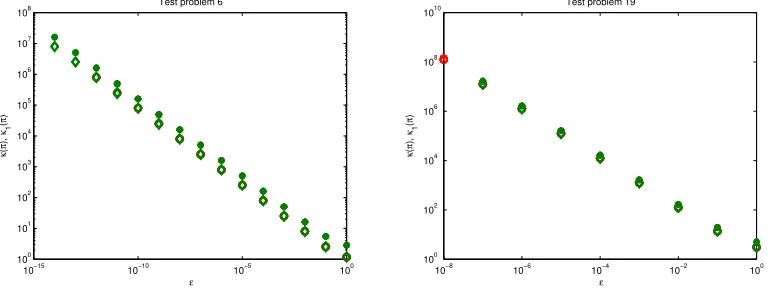
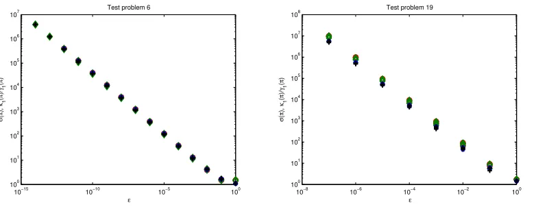
Figure 6.4 plots the condition numbers κ(π) and κ1(π) for a range of values of ǫ, and Figure 6.5 plots the value ofσ(π) and the ratio κ1(π)/γ1(π). For these problems we note that κ1(π)/γ1(π) ≈ σ(π), and the condition number κ(π)≈ 2κ1(π) grows like
p
(1/ǫ) for problem 6 and like 1/ǫ for problem 19. The stiffness ratioσ(π) has the same behavior (see 6.5).
10−15 10−10 10−5 100 100
101
102
103
104
105 Test problem 6
ε
NMAX
10−8 10−6 10−4 10−2 100 100
101
102
103
104
105 Test problem 19
ε
NMAX
Fig. 6.3. Circle (TWPBVPC(ON)), asterisks (TWPBVPC(OFF)), diamond (TWPBVPLC(ON)) and plus (TWPBV-PLC(OFF))) are the values of maximum mesh used by the codes with different values oftoland ofǫ.
10−15 10−10 10−5 100
100
101 102 103 104 105 106 107
108 Test problem 6
ε
κ
(
π
),
κ1
(
π
)
10−8 10−6 10−4 10−2 100 100
102
104
106
108
1010 Test problem 19
ε
κ
(
π
),
κ1
(
π
)
Fig. 6.4.Circle (TWPBVPC) and diamond (TWPBVPLC) are the values ofκ1(π), asterisks (TWPBVPC) and plus
(TW-PBVPLC) are the values ofκ(π).
the results obtained by the codes TWPBVPC and TWPBVPLC solving the problem with different values ofλ
and tol= 10−3, tol = 10−6 and tol= 10−9, using an initial mesh with N
S+ 1 mesh points. To be sure that the conditioning parameters obtained are stabilized we checked the value by running the code using a mesh doubled with respect to the final one and where we do not perform any grid refinement (the final mesh has
NF+ 1 points). In Table 6.1 we set the value of ST ABC equal to T if for the doubled mesh the value of κ(π) differs by less than 5 % from the value computed with the meshNF+ 1,ST ABCis set to F otherwise.
Only forλ= 3.5,3.51,3.513 do the codes give an output flag with a value of 0 andST ABC= T, for all the other values we have that the flag is−1. But in no cases do we accept a computed ‘solution’ when none exist. If we start the code with a starting mesh with a larger value ofNS, we see that for both the codes the value of
ST ABCis T when λ <= 3.51383. Forλ >3.51383, however, the number of mesh points in the final mesh can
be very high compared with the one used forλ≤3.51383. In particular TWPBVPC fails to give a solution for
λ≥3.513832, TWPBVPLC fails forλ≥3.513833, and for the solution given withλ= 3.513832 theST ABC flag is always F.
10−15 10−10 10−5 100
100
101 102
103 104 105
106
107 Test problem 6
ε
σ
(
π
),
κ1
(
π
)/
γ1
(
π
)
10−8 10−6 10−4 10−2 100
100
101 102 103 104
105 106 107
108 Test problem 19
ε
σ
(
π
),
κ1
(
π
)/
γ1
(
π
)
Fig. 6.5.Circle (TWPBVPC) and diamond (TWPBVPLC) are the values ofσ(π), asterisks (TWPBVPC) and plus (TWP-BVPLC) are the corresponding values ofκ1(π)/γ1(π).
some detail how this is done. Our codes can be considerably more efficient than other codes, due to the fact that we pay attention to the conditioning of the problem, and we have never accepted a ‘solution’ when none exists. However, for some problems, our conditioning parameters may converge rather slowly and we intend to examine this in detail in a future paper.
REFERENCES
[1] U. M. Ascher, R. M. M. Mattheij and R. D. Russell.Numerical solution of boundary value problems for ordinary differential equations, Classics in Applied Mathematics13. Society for Industrial and Applied Mathematics (SIAM), Philadelphia, PA, 1995. Corrected reprint of the 1988 original.
[2] Z. Bashir-Ali, J. R. Cash and H. H. M. Silva. Lobatto deferred correction for stiff two-point boundary value problems.Comput. Math. Appl.,36, no. 10-12, 59–69, 1998. Advances in difference equations, II.
[3] L. Brugnano and D. Trigiante. Tridiagonal matrices: invertibility and conditioning.Linear Algebra Appl.,166, 131–150, 1992.
[4] L. Brugnano and D. Trigiante. On the characterization of stiffness for ODEs.Dynam. Contin. Discrete Impuls. Systems,2, no. 3, 317–335, 1996.
[5] L. Brugnano and D. Trigiante. A new mesh selection strategy for ODEs.Appl. Numer. Math.,24, no. 1, 1–21, 1997. [6] L. Brugnano and D. Trigiante. Solving Differential Problems by Multistep Initial and Boundary Value Methods. Gordon &
Breach,Amsterdam, 1998.
[7] J. R. Cash. On the numerical integration of nonlinear two-point boundary value problems using iterated deferred corrections. II. The development and analysis of highly stable deferred correction formulae.SIAM J. Numer. Anal.,25, no. 4, 862–882, 1988.
[8] J. R. Cash and F. Mazzia. A new mesh selection algorithm, based on conditioning, for two-point boundary value codes.
J. Comput. Appl. Math.,184, no. 2, 362–381, 2005.
[9] J. R. Cash, F. Mazzia, N. Sumarti and D. Trigiante. The role of conditioning in mesh selection algorithms for first order systems of linear two point boundary value problems.J. Comput. Appl. Math.,185, no. 2, 212–224, 2006.
[10] J. R. Cash, G. Moore and R. Wright. An automatic continuation strategy for the solution of singularly perturbed nonlinear boundary value problems.ACM Trans. Math. Software,27, no. 2, 245–266, 2001.
[11] J. R. Cash and F. Mazzia. Algorithms for the solution of two-point boundary value problems. http://www.ma.ic.ac.uk/
~jcash/BVP_software/twpbvp.php.
[12] J. R. Cash and F. Mazzia. Hybrid mesh selection algorithms based on conditioning for two-point boundary value problems.
JNAIAM J. Numer. Anal. Ind. Appl. Math.,1, no. 1, 81–90, 2006.
[13] C. de Boor and H.-O. Kreiss. On the condition of the linear systems associated with discretized BVPs of ODEs.SIAM J.
Numer. Anal.,23, no. 5, 936–939, 1986.
[14] W. W. Hager. Condition estimates.SIAM J. Sci. Statist. Comput.,5, no. 2, 311–316, 1984.
[15] N. J. Higham. FORTRAN codes for estimating the one-norm of a real or complex matrix, with applications to condition estimation.ACM Trans. Math. Software,14, no. 4, 381–396 (1989), 1988.
[16] N. J. Higham. Accuracy and stability of numerical algorithms. Society for Industrial and Applied Mathematics (SIAM),
Philadelphia, PA, 1996.
[17] N. J. Higham and F. Tisseur. A block algorithm for matrix 1-norm estimation, with an application to 1-norm pseudospectra.
SIAM J. Matrix Anal. Appl.,21, no. 4, 1185–1201 (electronic), 2000.
[18] F. Iavernaro, F. Mazzia and D. Trigiante. Stability and conditioning in numerical analysis.JNAIAM J. Numer. Anal. Ind. Appl. Math.,1, no. 1, 91–112, 2006.
[19] P. Kunkel and V. Mehrmann. Differential-algebraic equations,Analysis and numerical solution. EMS Textbooks in
Table 6.1
Conditioning parameters, flags, number of mesh points in the initial constant mesh and number of mesh points in the final mesh for Problem 34
TWPBVPC(ON)
λ tol κ(π) κ1(π) γ1(π) σ(π) FL NS+ 1 ST ABC N+1
3.5 10−3
0.534E+02 0.366E+02 0.289E+02 0.130E+01 0 10 T 10
10−6
0.537E+02 0.368E+02 0.277E+02 0.136E+01 0 10 T 18
10−9
0.538E+02 0.368E+02 0.275E+02 0.137E+01 0 10 T 21
3.51 10−3
0.102E+03 0.701E+02 0.556E+02 0.128E+01 0 10 T 10
10−6
0.104E+03 0.712E+02 0.539E+02 0.134E+01 0 10 T 17
10−9
0.104E+03 0.712E+02 0.535E+02 0.135E+01 0 10 T 21
3.513 10−3
0.209E+03 0.144E+03 0.114E+03 0.126E+01 0 10 F 10
10−6
0.224E+03 0.154E+03 0.117E+03 0.132E+01 -1 10 T 19
10−9
0.224E+03 0.154E+03 0.115E+03 0.134E+01 -1 10 T 24
3.5138 10−3
0.105E+04 0.720E+03 0.549E+03 0.131E+01 -1 10 F 19
10−6
0.105E+04 0.720E+03 0.549E+03 0.131E+01 -1 10 F 19
10−9
0.105E+04 0.720E+03 0.549E+03 0.131E+01 -1 10 F 19
10−9
0.117E+04 0.801E+03 0.593E+03 0.135E+01 0 40 T 40
3.51383 10−3
0.214E+04 0.147E+04 0.112E+04 0.131E+01 -1 10 F 19
10−6
0.537E+04 0.369E+04 0.274E+04 0.135E+01 -1 10 F 37
10−9
0.537E+04 0.369E+04 0.274E+04 0.135E+01 -1 10 F 37
10−9
0.721E+04 0.495E+04 0.363E+04 0.136E+01 0 80 T 80
3.513831 10−3
0.225E+04 0.155E+04 0.118E+04 0.131E+01 -1 10 F 19
10−6
0.120E+05 0.823E+04 0.612E+04 0.135E+01 -1 10 F 37
10−9
0.120E+05 0.823E+04 0.612E+04 0.135E+01 -1 10 F 37
10−9
0.773E+04 0.531E+04 0.385E+04 0.138E+01 -1 80 T 10113
3.513832 10−3
* 10−6
* 10−9
*
TWPBVPLC(ON)
3.5 10−3
0.534D+02 0.366D+02 0.289D+02 0.130D+01 0 10 T 10
10−6
0.534D+02 0.366D+02 0.289D+02 0.130D+01 0 10 T 10
10−9
0.538D+02 0.368D+02 0.276D+02 0.137D+01 0 10 T 21
3.51 10−3
0.102D+03 0.701D+02 0.556D+02 0.128D+01 0 10 T 10
10−6
0.102D+03 0.701D+02 0.556D+02 0.128D+01 0 10 T 10
10−9
0.104D+03 0.712D+02 0.535D+02 0.135D+01 0 10 T 22
3.513 10−3
0.209D+03 0.144D+03 0.114D+03 0.126D+01 0 10 F 10
10−6
0.209D+03 0.144D+03 0.114D+03 0.126D+01 0 10 F 10
10−9
0.154D+03 0.116D+03 0.224D+03 0.133D+01 -1 10 T 21
3.5138 10−3
0.102D+04 0.700D+03 0.533D+03 0.131D+01 -1 10 F 19
10−6
0.102D+04 0.700D+03 0.533D+03 0.131D+01 -1 10 F 19
10−9
0.102D+04 0.700D+03 0.533D+03 0.131D+01 -1 10 F 19
10−9
0.117E+04 0.801E+03 0.593E+03 0.135E+01 0 40 T 40
3.51383 10−3
0.214D+04 0.147D+04 0.112D+04 0.131D+01 -1 10 F 19
10−6
0.537D+04 0.369D+04 0.274D+04 0.135D+01 -1 10 T 37
10−9
0.537D+04 0.369D+04 0.274D+04 0.135D+01 -1 10 T 37
3.513831 10−3
0.225D+04 0.155D+04 0.118D+04 0.131D+01 -1 10 F 19
10−6
0.354D+04 0.244D+04 0.176D+04 0.138D+01 -1 10 T 9217
10−9
0.354D+04 0.244D+04 0.176D+04 0.138D+01 -1 10 T 9217
3.513832 10−3
0.238D+04 0.164D+04 0.125D+04 0.131D+01 -1 10 F 19
10−6
0.146D+05 0.101D+05 0.729D+04 0.138D+01 -1 10 F 9217
10−9
0.146D+05 0.101D+05 0.729D+04 0.138D+01 -1 10 F 9217
10−9
0.146D+05 0.101D+05 0.729D+04 0.138D+01 -1 20 F 9729
10−9
* * * * -1 40 * *
3.513833 10−3
* 10−6
* 10−9
*
[20] R. M. M. Mattheij and G. W. M. Staarink. An efficient algorithm for solving general linear two-point BVP.SIAM J. Sci.
Statist. Comput.,5, no. 4, 745–763, 1984.
[21] R. M. M. Mattheij and G. W. M. Staarink. On optimal shooting intervals.Math. Comp.,42, no. 165, 25–40, 1984. [22] F. Mazzia, A. Sestini and D. Trigiante. The continous extension of the B-spline linear multistep metods for BVPs on
non-uniform meshes.Appl. Numer. Math.,59, no. 3-4, 723–738, 2009.
[25] F. Mazzia, A. Sestini and D. Trigiante. B-spline linear multistep methods and their continuous extensions.SIAM J. Numer. Anal.,44, no. 5, 1954–1973 (electronic), 2006.
[26] F. Mazzia, A. Sestini and D. Trigiante. BS linear multistep methods on non-uniform meshes.JNAIAM J. Numer. Anal. Ind.
Appl. Math.,1, no. 1, 131–144, 2006.
[27] F. Mazzia and D. Trigiante. A hybrid mesh selection strategy based on conditioning for boundary value ODE problems.
Numer. Algorithms,36, no. 2, 169–187, 2004.
[28] L. F. Shampine and P. H. Muir. Estimating conditioning of BVPs for ODEs. Math. Comput. Modelling,40, no. 11-12,
1309–1321, 2004.
Edited by: Pierluigi Amodio and Luigi Brugnano
Received: April 9, 2009