Density measurement of OH radicals in non-thermal plasmas by laser induced fluorescence and time-resolved absorption spectroscopy

(1)

U

NIVERSITY OF

T

RENTO

DEPARTMENT OFPHYSICS

THESIS

SUBMITTED TO THE

DOCTORALSCHOOL IN PHYSICS

BY

L

UCA

M

ATTEO

M

ARTINI

IN CANDIDATURE FOR THE DEGREE OF

PHILOSOPHIAE

DOCTOR

- DOTTORE DI RICERCA

D

ENSITY MEASUREMENT OF

OH

RADICALS

IN NON

-

THERMAL PLASMAS

BY LASER INDUCED FLUORESCENCE AND

TIME

-

RESOLVED ABSORPTION

SPECTROSCOPY

TUTOR: PROF. PAOLOTOSI

CO-TUTOR: DOTT. GIORGIODILECCE- CNR

(2)

(3)

(4)

(5)

Members of the doctoral thesis

committee

• Prof. Gino Mariotto (chair), Università degli Studi di Verona.

• Prof. Vittorio Colombo, Università degli Studi di Bologna.

• Prof. Giulio Monanco, Università degli Studi di Trento.

Trento, January 22nd_{, 2015}

(6)

(7)

Abstract

In the present thesis work, we have developed two different experimental setups for

the optical detection of the OH radical in discharges at atmospheric pressure. The first one

allows us to improve the time-resolved broband absorption spectroscopy. The main

ad-vances of the new set up are a better collimation of the UV light and a novel gating scheme.

They both significantly reduce the interference of the plasma-induced emission on the

ab-sorption measurement. The second setup is dedicated to an improved laser induced

fluor-escence experiment, which takes advantage of a novel multi-transition excitation scheme.

This permits the simultaneous measurements of both the OH density and its ground state

rotational temperature. In addition, we have developed a new rate-equation model to

ra-tionalize LIF spectra, by taking into account the electronic quenching, the vibrational and

rotational energy transfers, and the spatial profile of the laser beam. Finally, the electrical

power dissipated in the discharge was accurately measured.

(8)

(9)

Acknowledgements

I acknowledge my tutor Prof. Paolo Tosi for his support, patience, encouragement, and

scientific guidance throughout my PhD work. I also thank my co-tutor Dr. Giorgio Dilecce

for sharing his experience and ideas on optical diagnostics and plasma physics. Dr. Mario

Scotoni helped me with the laser source, and I am grateful to him for helpful advice and

inspiring discussions. I thank Dr. Matteo Franchi for helping me to develop embedded

sys-tems, and Dr. Marco Scapinello for working with me. Thanks are due to all the members

of the Atomic and Molecular Physics Group, for the great atmosphere and for making my

everyday life so enjoyable. Finally, I thank my parents and all my family for supporting

me. Especially, I would like to thank my wife for her encouragement, support and patience

during the Doctoral course.

(10)

(11)

Chapter 1

Introduction

1.1

Applications of atmospheric-pressure non-thermal plasmas

Laboratory plasmas are ionised gases, in the vast majority of the cases sustained by the

application of electric fields. The energy of the electric field is transferred, in the first

in-stance, to free electrons. It is subsequently distributed through collisions to the feedstock

molecules and their dissociation products. The sum of all possible excitation mechanisms

leads to the key aspect of non thermal plasmas (NTPs): the injected energy is not equally

distributed across all the species and their degrees of freedom. In particular, heating of the

gas can remain low (due to the large mass difference between the colliding electron and

molecule), while certain molecular states are highly excited. They promote bond breaking

and dissociation. Controlling and tailoring the non-equilibrium nature of the plasma is the

key to delivering the injected energy specifically to the bonds that are to be broken up. In

essence, NTP is an environment that is far from thermodynamic equilibrium conditions so

that conventional chemical processes are intensified and very high values of energy

effi-ciency can be achieved. Techniques based on atmospheric pressure non thermal plasmas are

used in several different fields. Important examples directly related to the present research

are the plasma reforming of CO2 for the production of solar fuels, the plasma destruction

of pollutants and the plasma medicine. Regardless of the specific application, the

quantitat-ive detection of the actquantitat-ive species generated in the plasma is an imperatquantitat-ive requirement for

the understanding of the plasma effects, because experimental molecular densities can be

(16)

2 CHAPTER 1. INTRODUCTION

compared with the results of model calculations, and eventually validate them. The

quan-tification of transient species is particularly challenging. My research activity in the last

three years, at the Doctoral School in Physics of the University of Trento, was devoted to

develop optical diagnostics in gaseous discharges for the detection of transient species, and

in particular of the OH radical.

1.1.1 Plasma reforming and solar fuels

Solar fuels are energy vectors that are produced from CO2 by using renewable energy

sources, i.e. solar energy, ultimately. The production of fuels and chemicals from

renew-able sources appears a promising way to store energy into value-added chemicals. Since

renewable energy sources are often intermittent, their exploitation requires storage systems,

ideally liquid chemicals that have high energy density. As the installed capacity of these

sources increases, so do issues related to load-balancing and to temporal and geographical

disparities between supply and demand. Implementation of quick-start systems for the

con-sumption of excess renewable energies could play a role in resolving these issues. This has

an incidental benefit in terms of the cost-effectiveness of the technology because the

elec-tricity generated during such periods of excess production is of relatively low cost.

Plasma-based systems are ideally suited to this task due to low inertia, low investment costs, and no

requirement for rare materials. At the same time reusing CO2 is a key element for curbing

green house gas (GHG) emissions [1].

NTPs have been explored for their capability to activate very stable molecules such as

methane and carbon dioxide at low temperature. In fact NTP are able to reform CO2 and

CH4to get value-added chemicals. Depending on the particular experimental set-up and the

specific operational features, different gaseous [2, 3], liquid [4, 5, 6] or solid chemicals [7]

are produced by the discharge in addition to the most abundant products CO and H2.

In our recent works [8, 9], our attempts to convert CO2 and CH4 in syngas (hydrogen

and carbon monoxide) and other value-added chemicals are presented. We show that a

par-tial control of the product selectivity can be achieved by modulating the electrical power

delivered to the discharge[8]. In addition, we investigated the catalytic effect of the

(17)

1.1. APPLICATIONS OF AP-NTPS 3

contribute to a better understanding of the fundamental processes involved. To this purpose,

the product branching ratio must be known as a function of discharge parameters. However,

if ones desire to investigate the detailed chemical mechanisms leading to the final products,

knowledge of the latter is not sufficient, and intermediate, transient species, such as CH₃, H

and OH, must be identified as they are chemical markers of specific reaction paths [10].

1.1.2 Plasma medicine

As outlined by Fridman in [11] “Plasma medicine embraces physics required to develop

novel plasma discharges relevant for medical applications, medicine to apply the

techno-logy not only in vitro but also in vivo testing and, last but not least, biotechno-logy to understand

the complicated biochemical processes involved in plasma interaction with living tissues”.

Radicals, in particular O-atoms and OH, are effectively generated in atmospheric pressure

discharges and they play a role in several plasma induced oxidation processes [12, 13].

For this reason radical diagnostics is a key point for the rapidly developing field of plasma

medicine[14]. In addition, OH measurements in test cases are of interest for comparison to

recent model calculations [15].

1.1.3 Plasma abatement of pollutant

Nowadays environmental protection is an important issue. Exhausts from mobile and

stationary sources pollute the air with a variety of dangerous substances for the human

health and the ecological life. Volatile organic compounds (VOCs) are an important group

among these pollutants. VOCs play an important role at global level (global warming

pro-moters), at regional scale (acid rain propro-moters), but especially at local scale, directly

affect-ing human health given that several VOCs are carcinogens. Also in the everyday indoor

en-vironments, organic compounds can be detrimental for human health. NTPs offer interesting

opportunities in the field of air-cleaning systems. There is a clear opportunity for NTP

tech-niques to be employed for the activation and dissociation of the feedstock molecules[16].

Reactive oxygen species (ROS), such as O, OH, O3, H2O2, HO2 and O2(a1∆g), play an

important role in pollutants remediation. Indeed, VOCs destruction mainly proceeds via

(18)

4 CHAPTER 1. INTRODUCTION

of oxidant species, and their quantitative detection is a critical issue to improve the

perform-ance.

1.2

Optical spectroscopy diagnostics of discharges at

atmospheric pressure

Spectroscopic diagnostics are particularly suitable to estimate quantities such as gas

temperature, electron density, electric field and density of transient species. The main optical

diagnostic techniques are: optical emission spectroscopy (OES), laser induced fluorescence

(LIF), and absorption spectroscopy (AS). OES is the simplest technique and thus it is widely

used. Unfortunately, it provides information only about excited species, which depend in a

complex and indirect way on the corresponding ground state populations. Molecules in their

ground state can be instead detected either by AS or by LIF. AS is cheap, provides absolute

outcomes, but its spatial and temporal resolution is low [17, 18].

Laser induced fluorescence (LIF) is the best technique if sensitivity, time and space

resolution are a crucial requirement [19]. LIF, however, needs a calibration because the

outcome is not absolute. In addition, the LIF signal depends on collisional processes of the

excited state, and therefore a detailed model is necessary to rationalise the experimental

(19)

Chapter 2

Time-resolved broad-band

absorption spectroscopy

In absorption spectroscopy, the light radiation passes through the plasma, and the

modi-fication of the spectrum as a function of the wavelength of the incoming light by absorption

and scattering is measured. Absorption spectroscopy is the technique of choice to get the

absolute density of molecules in their ground state. When dealing with plasma-mediated

processes, absorption can be achieved by simply using an incoherent broadband light source

much brighter than the plasma itself, like broad-band xenon or deuterium lamps [20].

Un-fortunately, not all the spectral regions can be covered by broadband sources. When no

broadband light sources are available,self-absorptioncan be used. In this case the plasma itself can be used as source [21]. Resonant transitions can be also achieved by using tunable

laser-based systems [22].

Various types of arrangements and techniques have been developed in the past years in

the field of non-thermal atmospheric pressure plasmas or other similar environments (like

flames or plasma activated flames), such as resonant absorption [17], broad-band absorption

spectroscopy (BBAS) [18, 23], cavity enhanced absorption spectroscopy (CEAS) or cavity

ring-down spectroscopy (CRDS) [24, 25, 26, 27]. An example of the application of

absorp-tion spectroscopy in plasma environments is the detecabsorp-tion of CF₂ by using a Xe arc lamp

as a light source in Ar/fluorocarbon mixtures [28]. As far as tunable laser diode absorption

(20)

6 CHAPTER 2. TR-BBAS

sure plasma jet operating at13.56MHz in argon with small admixtures of air in a multi-pass

cell. Ar(1s5)metastable density measurements were carried out by Belostotskiyet al. [30]

in a pulsed dc argon micro-plasma discharge by using diode laser absorption spectroscopy.

The populations of the excited Ar atoms were studied by Penacheet al. [31] using diode laser atomic absorption spectroscopy. Also Niemiet al. [32] measured metastable He with the same technique.

In recent years the development of cheap, broad-band, very stable near-UV sources

(UV-LED) has increased the interest for the BBAS technique. In fact, many radicals have

strong electronic transition in the near-UV range. An example is the OH radical and its

A2Σ+ ← X2Π transitions that were used by Dilecce et al. [18] and Bruggemanet al.

[33] for absolute temperature and concentration measurements. In the following sections I

describe our new attempt to improve the TR-BBAS technique [23].

2.1

Broad band absorption spectroscopy: principles and

applic-ation to OH

2.1.1 Basics nomenclature in light-matter interaction

When molecules undergo an electronic transition between an upper leveljand a lower

leveli, a spectral line is emitted. The wavelengthλji of the emitted line is proportional to

the energy gap between the two levels:

νji=

Ej−Ei

h λji =

c νji

,

wherec indicates the speed of light. If the transition is spontaneous the variation of the

population of the upper levelnjis proportional to the population density and to the Einstein

coefficient of spontaneous emissionAji:

−dnj

dt =Ajinj.

When the emission of photons is induced by the radiation, one gets

−dnj

(21)

2.1. BBAS: PRINCIPLES AND APPLICATION TO OH 7

The induced emission is proportional to the level population, the Einstein coefficientBji

and to the spectral radiant energy densityξν, like its inverse process, the absorption:

−dni

dt =Bijξνni. (2.1)

The Einstein coefficients for absorption and induced emission are related by:

giBij =gjBji,

wheregiandgjare the statistical weights of the lower and higher level, respectively.

2.1.2 Broad band absorption

The BBAS technique consists in the measurement of changes of the spectral radiance

I(x, ν)induced by the absorption process along the optical path[20]. Radiation absorption

within a media can be described by introducing a wavelength-dependent absorption

coeffi-cientκ(x, ν)defined as

dI(x, ν) =−κ(x, ν)I(x, ν)dx (2.2)

that represents the variation of the spectral radianceI(x, ν)along the directionxby a thin

slabdxof absorbing medium. The unit ofκ(x, ν)is m−1and the spectral radianceI(x, ν) unit is W s−1m−2sr−1. By the spatial integration of Eq. 2.2 along the lengthl(the optical path inside the discharge) one gets the well known Lambert-Beer law:

I(l, ν) =I(0, ν) e− Rl

0κ(x,ν)dx _(2.3)

Given the central frequency of a certain transitionνji, the line absorption coefficient can

be written as a function of the transition line shape functionL(ν −νji), with its integral

respect to the frequency normalised to one, and the integrated line absorption coefficient

κL(x, νji):

κji(x, ν) =κL(x, νji)L(ν−νji),

Z −∞

+∞

L(ν−νji) dν = 1.

(22)

8 CHAPTER 2. TR-BBAS

hξν it becomes equal to the right-hand side of Eq. 2.2 after the integration of the absorption

coefficientκ(x, ν):

Bjiξν(νji)nj∆xhνji=Iν(νji) ∆x

Z −∞

+∞

κ(x, ν−νji)dν

=κL(x, νji)Iν(νji) ∆x.

Considering the case of collimated radiation, the radiance and the radiant energy density are

related by

ξ(ν) = 1 cI(ν),

changing the coefficients unit from frequency to wavelength one gets:

κL(x, λji) =

hλji

c Bjinj.

Considering the cross-sectionσjias the absorption coefficient divided by the density of the

species in the lower statejwe have

σji(x, λ) =

κji(x, λ)

Nj(x)

= κ

L₍_{x, λ}

ji)L(λ−λji)

Nj(x)

=σ_jiLL(λ−λji).

Assuming that the spatial dependence is only in theNj(x)term, one gets

σL_ji≈ κ

L₍_λ ji)

Nj(x)

= hλji

c Bji. (2.4)

The Lambert Beer law (Eq. 2.3) for a single molecular band withNj(x) = njN(x),

where nj is the fractional population of the rotational level involved in the transition j,

becomes:

Iλ(l, λ) =Iλ(0, λ) e−

Rl

0N(x)dx

P

jnjσjiLL(λ−λji)_. _(2.5)

2.2

Time-resolved broad-band absorption spectroscopy

experi-mental set-up

The TRBBAS set-up is composed of two main parts: the broad-band light source and

(23)

2.2. TR-BBAS SET-UP 9

2.2.1 Light Source

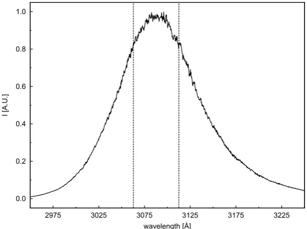
The light source used to probe the OH molecule is a UV-LED

(UVTOP-310-TO39-BL, SET) with a peak-emission wavelength at3089Å and a full width at half maximum

(FWHM) of89Å (Figure 2.1). The UV-LED is housed in a TO-39 package and equipped

with a ball lens with a focal length of≈18mm. The maximum LED forward current in cw

mode is30mA, but it can be increased to200mA in pulse mode (at1kHz,1%duty cycle).

To inject the UV-light into the discharge gap it is crucial to collimate the LED radiation.

A good collimation permits a multiple pass configuration and the possibility to add a spatial

0.0 0.2 0.4 0.6 0.8 1.0

2975 3025 3075 3125 3175 3225

I [A.U.]

wavelength [Å]

Figure 2.1:Measured spectral profile of the UVTOP-310-TO39-BL (SET) UV-LED. The vertical lines set the

range of OH absorption.

filter after the discharge to decrease the amount of spontaneous emission radiation reaching

the detector. Unfortunately, the LED is not a point-source of light, and the quality of the

beam obtained using a single-lens collimation system is poor, i.e. the beam remains well

collimated only over a short distance (in the order of≈100−200mm [18]). In this

con-dition, it is possible to get only a single-pass configuration through the discharge area (that

is35mm wide). On the other hand, the rejection of the spontaneous emission is achieved

(24)

10 CHAPTER 2. TR-BBAS

Figure 2.2:Scheme of the LED collimation arrangement. The LED has a ball lens on top. The skimmer is made

of polished nickel; its internal walls are partially reflective. The200µm nozzle of the skimmer acts

as a small size source allowing a good collimation by the50mm focal length collimation lens [23]

the spontaneous emission with spatial filters requires putting the detector centimetres away

from the discharge. Increasing the beam collimation corresponds to a significant increase

of the spontaneous emission rejection, as well as the possibility to lengthen the optical path

inside the plasma.

The solution adopted is presented in Figure 2.2, where we put the UV-LED inside a

skimmer made of polished nickel. The skimmer’s walls help to canalisethe UV-light to the 200µm exit bore that is placed in correspondence of the LED ball lens focal point.

Af = 50mm lens is used to collimate the light exiting from the nozzle. The resulting

beam remains well collimated for a distance of≈ 500mm with a section in the order of

1−2mm2. Thanks to the better beam collimation we could adopt a two-pass configuration inside the discharge and we could add two irises in order to spatially filter the spontaneous

emission. Of course the disadvantage is that an increasing beam collimation decreases the

beam intensity.

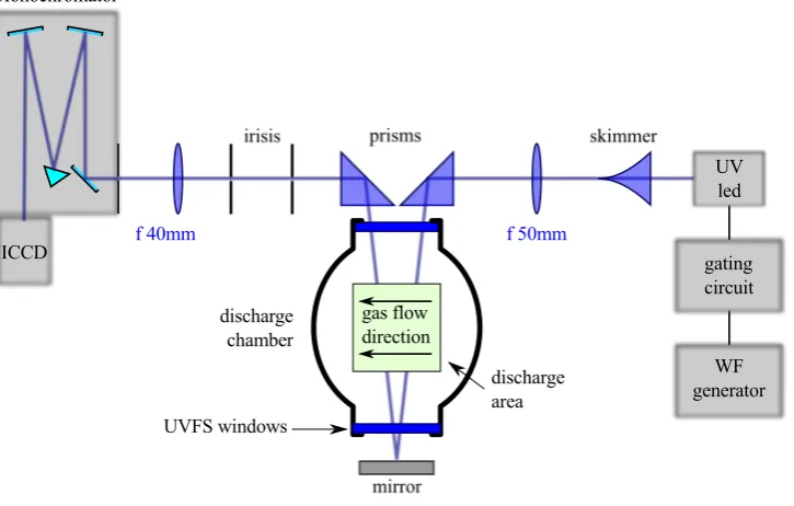
Figure 2.3 shows the schematic representation the TR-BBAS apparatus. The light travels

inside the discharge area perpendicular to the gas flux. The total absorption length is70mm

The UV-LED driver is an home-made gateable current source circuit made of fast JFET

transistors, with a maximum output current of160mA and a minimum gate time of500ns.

(25)

2.2. TR-BBAS SET-UP 11

Figure 2.3:Schematic representation of TR-BBAS apparatus. The UV-LED beam is injected in the discharge

area with a double pass configuration. Irises serve as spatial filters in order to stop the spontaneous

emission emitted by the discharge. Thef = 40mm lens matches the incoming UV-beam to the

(26)

12 CHAPTER 2. TR-BBAS

2.2.2 Light Detectors

The first detection setup D1 is based on a140mm focal length monochromator

(mi-croHR, Jobin-Yvon) equipped with a1200gr mm−1 300nm blaze grating with a 100µm input slit. The light detector is a charge coupled device (CCD) (GARRY 3000, Ames

Photonics). This device is non-cooled, non-intensified, gateable3000elements linear CCD

array. The second detection setup D2 is composed of a300mm focal length monochromator

(Shamrock 303i, Andor) equipped with a1200gr mm−1300nm blaze grating,70µm input slit. The detector coupled to the Shamrock 303i is a cooled,1024×1024pixel, intensified

CCD (ICCD) (DH334T-18U-03, Andor).

2.2.3 Discharge Design

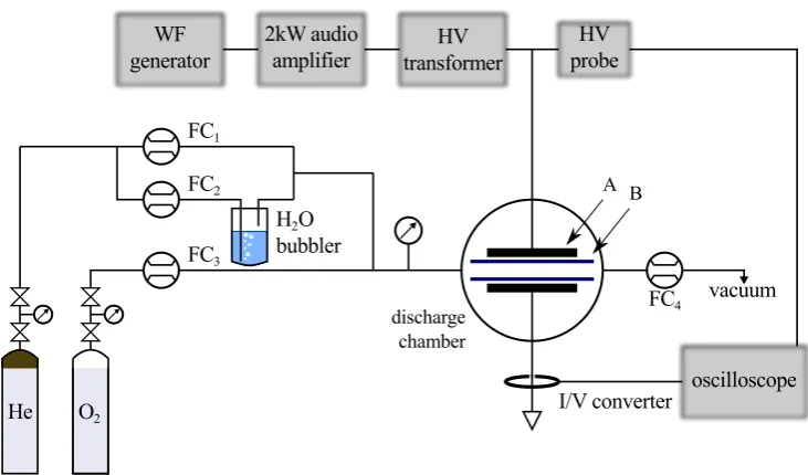
Figure 2.4:Schematic representation of the DBD set-up.F C1−4: mass flow controllers; A:35×35mm2copper

electrodes; B:0.7mm thick alumina plates.

A schematic representation of the discharge gas feed and electrical apparatus is shown

in Figure 2.4. The discharge set-up is composed of two main components, the plasma power

(27)

2.2. TR-BBAS SET-UP 13

Discharge configuration and gas feed

The dielectric barrier discharge used is a parallel plate configuration composed of35×

35mm2copper electrodes. Two0.7mm thick alumina plates are used as dielectric barriers. Two inter-electrode gaps have been used (4.5mm and2.0mm). With these two

configura-tions the electrode surface is12.25cm2 and the discharge volume 5.50cm3 and2.45cm3 for4.5mm and 2.0mm, respectively. The discharge gas feed is composed of three

separ-ate gas lines: a pure He (99.995%purity) carrier controlled by a1000sccm full scale mass

flow controllerF C1(1179B, MKS); a pure He (99.995%purity) flow injected in a bubbler

filled with distilled water, whose temperature is measured with a typeKthermocouple, con-trolled by a500sccm full scale mass flow controllerF C2 (1179A, MKS); and a pureO2

(99.995%purity) line controlled by a10sccm full scale mass flow controllerF C3(1179A,

MKS). Another 5000sccm full scale mass flow controller F C4 (1179A, MKS) is placed

in between the discharge chamber and the4m3h−1 membrane pump. Thanks toF C4 the

pressure inside the discharge chamber is kept at a constant value20torr above atmospheric

pressure, in order to prevent air to penetrate inside the discharge chamber. The water partial

pressure inside the discharge chamber is described by the equation:

PH2O=P

vap H2O(T)

φ2

φ1+φ2+φ3

,

where P_Hvap

2O(T) is the water vapour pressure at the temperature T, φ1 is the flux of the

He carrier, φ2 is the He flux injected in the bubbler and φ3 is the O2 flux, as described

in [34, 35]. The total flux injected into the discharge chamber is kept at a constant value of

500sccm during measurements. Mass flow controllers are driven by a computer controllable

multi-gas controller (647B, MKS).

Power supply and electrical diagnostic

The high-voltage (HV) power supply is composed of a wave form generator (33220A,

Agilent) that generates a sinusoidal signal amplified by a2kW bridged class-D audio

amp-lifier (UCD2k OEM, Hypex). The amplified low-voltage signal is converted in a HV

stim-ulus Vs by using a HV transformer (Al-T1000.7-P10, Amp-Line). The secondary coil of

(28)

14 CHAPTER 2. TR-BBAS

a HV high bandwidth (DC -75MHz) probe (P6015A, Tektronix) that is used as a voltage

monitor. The second discharge electrode is connected directly to the ground and a high

bandwidth (200Hz - 500MHz) I/V converter (CT-01-b, Magnelab) is placed around the

wire that connects the reactor to the ground. Signals acquired by the voltage and current

probes are digitalised and recorded by a four-channel4GSps 600MHz bandwidth digital

signal oscilloscope (DSO) (Infiniium 54831B, Agilent).

2.2.4 PC based control program

I wrote a program by using LabWindows/CVI (National Instruments) to control the

discharge gas feed apparatus, plasma power supply and to record the spectrum acquired by

the CCD/ICCD. A schematic representation of the connection between the apparatus and the

PC is presented in Figure 2.5. The program initialises the waveform generators in order to

Figure 2.5:Schematic representation of the pc-based control system. WFG 1-2: waveform generators

synchron-ised in frequency and phase by sharing the10MHz external time-base reference. Black lines: analog

and digital signals; Blue lines: UV-LED light signal; Green line: gas feed connection.

generate the gates for the UV-LED and for the detector, sets amplitude, frequency and duty

cycle of the sinusoidal signal that drives the discharge. For every mixture of He−O₂−H₂O,

(29)

2.3. MEASUREMENT STRATEGY 15

pressure inside the discharge chamber. Absorption measurement requires the acquisition of

the light generated by the UV-LED interacting with the discharge. In order to avoid the

influence of the light source fluctuations or changes in the external light background, each

acquisition of an absorption spectrum is followed by that of the UV-LED light signal, i.e.

with the plasma switched off. Several spectra were taken in order to increase the statistics

and to achieve a better detection limit.

2.3

Measurement strategy

The transitions involved in the absorption belong to the (0,0) band of the OH3064Å

sys-tem,A2Σ+←X2Π. In order to eliminate measurement baseline drift, LED low-frequency intensity fluctuations, and to reduce as much as possible the spontaneous emission from

the plasma, we adopted a time-resolved detection strategy for the TR-BBAS. The timing

−4.0 −2.0 0.0 2.0 4.0

0 4 8 12 54 58 62 66

Voltage [kV]

Led−on period [A.U.]

Time [ms]

Led−on period discharge ON Led−on period discharge OFF

Figure 2.6:Red line: CCD/ICCD gate and LED pulsing for the TR-BBAS scheme, Led-on period discharge

OFF provides the reference (without absorption) light intensity. Black line: sinusoidal stimulus

applied to the discharge.

scheme of a TR-BBAS experiment is shown in Figure 2.6. We modulate the sinusoidal

(30)

16 CHAPTER 2. TR-BBAS

During the sine wave burst, the plasma switches on (the duration of the burst is defined by

the number of burst times the period of the sine waveTON = 10ms). After the burst of

sine waves, the waveform generator output goes to zero for a timeTOF F = 90ms, and

consequently the plasma switches off. The sum ofTON andTOF F defines the total period

T of the on-off cycle, which isT = 100ms. The OH concentration is probed by

acquir-ing the absorption spectrumI_λM(l, λ)at the end of theTON period, for a total duration of

T_LEDON = 300µs (the same gate was applied to the UV-LED driver and to the CCD-ICCD gate). A further acquisition is carried out 50ms after the first one in order to record the

LED profileI_λM(0, λ) when the [OH] becomes negligible[34, 35, 18]. The resulting gate sequence is a combination of the sine-wave burst at10Hz and the LED/detector-gate at

20Hz. Gates are generated by two waveform generators, whose synchronisation is ensured

by sharing the10MHz external time-base reference. In this way, the two devices are

syn-chronised in phase and frequency.

The gate configuration just described was used in conjunction with the D1 scheme based

on the non-cooled, non-intensified, gateable linear CCD array. In this case, the spontaneous

emission rejection was achieved by using spatial filters (irises) placed in between the

dis-charge area and the monochromator. The rejection of the spontaneous emission can be

fur-ther increased by using the improved detection scheme D2, which is based on the

synchron-isation of the ICCD acquisition with respect to the periodical null value of the discharge

current (see Figure 2.8), i.e. when the spontaneous emission is minimal. For comparison, in

the scheme D1, the signal is acquired continuously during the LED gate, i.e. for each value

of current.

Spontaneous emission is detrimental for BBAS because, in many cases, it is much

more intense than the absorption signal. Besides the OH concentration value, it can also

affect the temperature estimate. We notice that the spontaneous emission is generated by

the A2_Σ+₍_υ_{= 0)} _→ _X2_{Π (}_υ_{= 0)} _{band, that is the same interested by the absorption}

A2Σ+(υ= 0) ← X2Π (υ= 0). Bruggemanet al. in [33] proposed to calculate the ab-sorption spectrum of OH subtracting the spontaneous emission from the transmitted LED

light (which of course contains also the plasma spontaneous emission). However, if the

(31)

2.3. MEASUREMENT STRATEGY 17

by a strong systematic error. For these reasons, we chose alternative strategies in order to

decrease the incidence of spontaneous emission in the measurement:

• using light sources with an adequate radiant energy density, much larger than the

spontaneous emission. In this way, it is possible to adopt short CCD gates and in turn

to acquire less spontaneous emission radiation.

• rejecting the spontaneous emission that travels from the discharge to the detector by

stopping all the radiation that is not collimated with the UV-LED beam.

• adopting a multi-pass strategy to increase the optical path, i.e. the absorbance signal.

Finally, we emphasise the importance of the light source that has to be gateable and well

collimable.

During theTONperiod the spontaneous emission intensity is not constant, and it follows

the time dependence of the voltage. We measure the spontaneous emission intensity versus

time using the D2 configuration. The gate scheme is equal that presented in Figure 2.6, but

the LED is always kept in the off state. In this way, duringTON the spontaneous emission

plus background is recordedI_λSE(λ), and duringTOF F only background lightI_λBG(λ)is

acquired. We used a5µs gate for the ICCD.I_λSE(λ)andI_λBG(λ)are obtained by averaging 2000single ICCD acquisitions. The integral respect to the wavelength of

ISE(λ) =IλSE(λ)−IλBG(λ),

is used to quantify the spontaneous emission intensity. The results, taken at various delay

times with respect to the excitation voltage, are presented in Figure 2.7. The spontaneous

emission reaches the maximum value when the current flowing inside the discharge is at

its largest values. On the other hand, when the current is zero, the spontaneous emission is

negligible (that happens two times every excitation voltage period). The spontaneous

emis-sion is related to exited OH molecules that are generated by the plasma when the current

increases rapidly inside the voltage excitation period. These excited molecules decay

radi-atively to the ground state rapidly inside aVs semi-period, while the ground state [OH] is

(32)

18 CHAPTER 2. TR-BBAS 0.00 0.25 0.50 0.75 1.00

Spontaneous Emission [A.U.]

−8.0 −4.0 0.0 4.0 8.0

−0.03 −0.02 −0.01 0.00 0.01 0.02 0.03

−8.0 −4.0 0.0 4.0 8.0 Voltage[kV] Current[10 −2 A] Time [ms]

Figure 2.7:Top:Rλmax

λmin ISE(λ)dλin function of time, points are interpolated with a spline. Bottom: current

(red line) and voltage (black line) in function of time.

dependence of the spontaneous emission, we decided to improve the spontaneous emission

rejection only by changing the gates sequence of the acquisition.

The image intensifier (multi-channel plate, MCP) coupled with a cooled CCD, permits

to use the MCP as an electrical shutter. Taking advantage of theintegration on chip(IOC) function of the ICCD, we realised the possibility to gate the MCP several times during

a single CCD acquisition. In this way, it is possible to sampleI_λM(l, λ) when the spon-taneous emission is negligible, for a10µs time interval immediately before the discharge

current increases. During the following15µs, the MCP is switched off, thus avoiding to

detect the spontaneous emission (25µs is aVs semi-period). The CCD signals (IλM(l, λ)

andIM

λ (0, λ)) are then acquired by switching the MCP on and off14times during a single

400µs CCD-LED gate. A representation of the CCD-LED and MCP gates together with

theI-V characteristic of the discharge are shown in Figure 2.8. The resulting effective gate

time for the signal acquisition decreases from300µs in the case of detection system D1 to

140µs in the case of D2, at the expense of the signal to noise ratio. A comparison between

theISE(λ) values acquired with and without the MCP gating is presented in Figure 2.9.

(33)

2.3. MEASUREMENT STRATEGY 19

−5.0 −2.5 0.0 2.5 5.0

−1.0 −0.5 0.0 0.5 1.0

LED Gate [V]

Detector Gate [V]

−8.0 −4.0 0.0 4.0 8.0

9.6 9.7 9.8 9.9 10.0

−8.0 −4.0 0.0 4.0 8.0

Voltage[kV]

Current[10

−2

A]

Time [ms]

Figure 2.8:Top: Detail of the gating at the end of the discharge packet, the MCP gating (blue line) is for

detection system D2 only. It is open (negative level) in the null discharge current intervals. The

black line is the LED-CCD gate. Bottom: current (red line) and voltage (black line) in function of

(34)

20 CHAPTER 2. TR-BBAS

0.993 0.994 0.995 0.996 0.997 0.998 0.999 1.000 1.001 1.002 1.003

3050 3060 3070 3080 3090 3100 3110 3120

I

M(l,

λ

) / I

M(0,

λ

)

wavelength [Å]

absorption MCP−gating OFF absorption MCP−gating ON spontaneous emission MCP−gating OFF spontaneous emission MCP−gating ON

Figure 2.9:Spontaneous emission (blue line) and transmittance spectrum (black line) in function of wavelength

for the spatial filtering strategy. The red and yellow lines are the transmittance spectrum and the

spontaneous emission, respectively, for the spatial filtering plus MCP gating strategy. Dashed lines

(35)

2.3. MEASUREMENT STRATEGY 21

However, although effective in the case of the OH detection in a DBD, this strategy cannot

be applied in general, in particular either to short living molecule or discharges where the

excitation period is short compared to the life time of the states responsible of spontaneous

emission.

For both the measurement configurations, (in order to decrease the measurement noise)

the quantitiesI_λM(l, λ)andI_λM(0, λ)are obtained by averaging10000gate CCD signals.

2.3.1 Fit of the experimental data

Our experiment is based on transitions of the3064Å system(0,0)band. The outcomes

are values of the spectral radiance when the discharge is on and off,I_λM(l, λ)andI_λM(0, λ), respectively. These two quantities and the modelled spectral radianceIλ(l, λ)(Eq. 2.5) are

related by the equations

I_λM(l, λ) = Z +∞

−∞

Iλ(l, λ0)S(λ0−λ)dλ0, (2.6)

I_λM(0, λ) = Z +∞

−∞

Iλ(0, λ0)S(λ0−λ)dλ0, (2.7)

whereS(λ)is the spectrometer instrumental function, that of course is different for the two

detection systems. In the case of the second detection setup D2, the instrumental function

is presented in Figure 2.10. The instrumental function was recorded by putting a He−Ne

calibration lamp (6034, Newport) in front of the spectrometer slit entrance. The optimum slit

width was chosen in order to have the maximum signal to noise ratio with a good spectral

resolution [18]. The entrance input slit widths used were 100µm and 70µm in the case

of detection setup D1 and D2, respectively. The transmittance spectrum is defined as the

ratio between the spectral radiance in the discharge-on condition (Eq. 2.6) and the spectral

radiance in the discharge-off condition (Eq. 2.7).

I_λM(l, λ) I_λM(0, λ) =

Z +∞

−∞

e−lNaveP_iniσiLL(λ 0₋_λ

i)_SN₍_λ0₋_λ_)d_λ0_. _(2.8) In the limit of a narrow instrumental function, i.e. narrow with respect to the wavelength dependence of the light source,Iλ(0, λ)can be brought out of the integral sign in Eq. 2.8.

The termNaverefers to the average particles density along optical path (l= 70mm)

Nave =

1 l

Z l

0

(36)

22 CHAPTER 2. TR-BBAS

0.0 0.2 0.4 0.6 0.8 1.0

2947 2952 2957 2962 2967 2972 2977 2982 2987

I [A.U.]

wavelength [Å]

Figure 2.10:Detection system D2 instrumental function for a70µm input slit width.

andSN₍_λ₎_{is the normalised instrumental function of the spectrometer}

SN(λ) = _R₊_∞S(λ)

−∞ S(λ)dλ .

The termsniσLi L(λ−λi)in the sum over theitransitions of the(0,0)band are calculated

starting from the LIFBASE spectral simulation program [36]. Given a certain temperature

and line shape function, LIFBASE calculates a spectrum normalised to the peak absorption

line (only proportional toniσLi L(λ−λi)). The line shape function used in our simulations is

given by a Doppler plus pressure broadening profile (Figure 2.11). The pressure broadening

is taken from [37], and its value of3.5GHz atm−1 at298K is assumed to be the same for all rotational levels.

Starting from a set of simulated transition spectra, corresponding to various

temper-atures, and by comparing them with the experimental data, it is possible to estimate the

absolute mean concentration of OH radical along the optical path.

We wrote a C program that fits Eq. 2.8 on the experimental data. An example of the

measured transmittance TM₍_λ_{) =} IλM(l,λ)

IM λ (0,λ)

is shown in Figure 2.12. It is visible an

an-omalous negative baseline that deviates from the expected value of a transmittance spectra

(37)

2.3. MEASUREMENT STRATEGY 23

0.0 0.2 0.4 0.6 0.8 1.0

3060 3070 3080 3090 3100 3110 3120

I [A.U.]

wavelength [Å]

sintetic spectrum convoluted spectrum

Figure 2.11:Black line: simulated transmittance spectrum, the line shape function is given by a Doppler plus

pressure broadening profile. Red line: simulated transmittance spectrum convoluted with the

in-strumental function of detection system D2.

0.990 0.992 0.994 0.996 0.998 1.000 1.002

2920 2960 3000 3040 3080 3120 3160 3200 3240

I

M(l,

λ

)/I

M(0,

λ

)

wavelength [Å]

TM(λ) original TM(λ) corrected baseline fit

Figure 2.12:Black line: experimental transmittance spectrum. Blue line: baseline best fit of a4th

order

(38)

24 CHAPTER 2. TR-BBAS

the media along the optical path during the plasma-on condition, which in turn creates an

an-omalous transmittance signal. A change in the refractive index of the medium corresponds

to a shift in the wavelength of the UV-LED profile. In order to eliminate this spurious effect

we fitted the baseline with a4th order polynomial function (the blue line in Figure 2.12) and we subtracted it from the experimental transmittance. The result is the red graph in

Fig-ure 2.12 where only the transmittance spectra of theA2Σ+(υ= 0)← X2Π (υ= 0)band is present.

We then re-normalise the LIFBASE spectrum to the value required in Eq. 2.8 by taking

an isolated line, the P1(2) one, and normalising its spectral integral ton(N=2, F1e)σ

L P1(2),

us-ing formula Eq. 2.4 with the absorption coefficient taken from LIFBASE database.n(N=2, F1e) is the population of the rotational sublevel N = 2, F1e (J = 2.5), parity e at a given

rotational temperature [18, 38] (see Appendix B for the nomenclature of transitions and

rotational levels).

Given a OH density value, all theniσLi L(λ−λi) transitions of the (0,0) band were

multiplied by the average OH density and the optical path length. After computing the

ex-ponential term inside the integral of Eq. 2.8 we calculated the circular convolution with the

monochromator instrumental function. In order to estimate the right value of the OH

con-centration all these calculation were carried out using a multidimensional nonlinear

last-squares fitting tool written using the GNU Scientific Library [39]. After the baseline

sub-traction,150points of the experimental transmittance spectrum were used to fit the model

of Eq. 2.8 to the experimental spectrum. This allows us to estimateNave (the OH density)

and the wavelength offsetωo between the experimental data and the model. The program

minimises the squared residuals of then = 150functionsfi via the parametersNave and

ωo

Φ (Nave, ω0) =

1

2kF(Nave, ω0)k

2₌

= 1

2χ

2₌ 1

2

n

X

i=1

T(Nave, ω0, λi)−TM(λi)

2

σ2

i

, (2.9)

whereσiare the errors associated with each of the150points of the transmittance spectrum

TM(λi). We estimated the errors by acquiring the spectrumTM(λi)with the plasma off

(39)

2.3. MEASUREMENT STRATEGY 25

1e−04 1e−03

0 1000 2000 3000 4000 5000 6000 7000 8000 9000 10000

standard deviation of I

s

/I0

number of acquisitions

T_CCD = +25 °C TCCD = −10 °C

TCCD = −25 °C

Figure 2.13:Standard deviation of150points of the experimental spectrum in function of the number of the CCD acquisition. Measurements were taken using detection system D2, keeping the discharge

always in the off-condition, at three different CCD temperatures.

Figure 2.13, the standard deviation of the n = 150 points used to fit the experimental

plot is presented as a function of the number of acquisitions of TM₍_λ

i) (i.e. for every

acquisition ofI_λM(l, λ) andI_λM(0, λ)) carried out with detector scheme D2 (300µs CCD and MCP gate). We computed the standard deviation for three temperature values of the

CCD, which works in a quasi-saturated regime. Figure 2.13 shows that for achieving a lower

uncertainty in the transmittance spectrum, the CCD has to be kept at room temperature

or even higher temperatures. We decided to set the temperature of the CCD toTCCD =

15◦C. In this condition, the standard deviation of the150points is around1.5×10−4after averaging10000 TM measurements. We decided to associate to every measured point of the transmittance spectrum an error equal to3×σi ≈5×10−4. The fitting program starts

from initial guesses for OH densityN_ave0 , and the wavelength offsetω₀0. Then it evaluates the term:

φ(N_avep , ω₀p) =kF N_ave0 +N_avep , ω0₀+ω₀p k ≈

≈ kF N_ave0 , ω₀0

(40)

26 CHAPTER 2. TR-BBAS

whereNavep andωp₀ are the proposed steps, andJ(Navep , ωp₀)is the Jacobian defined as:

Jij(Navep , ω p

0) =

1 σi

∂(T(Nave, ω0, λi))

∂xj

.

In the Jacobian,xjare the parameters to be fit, and the algorithm tries to minimise the linear

systemkF N0

ave, ω00

+J(Navep , ωp0)kusing the Levenberg-Marquardt [40]. The terms of

the jacobian matrix are computed numerically using a two-point numerical derivative. Best

fit parameter errors are inferred from the covariance matrix. Figure 2.14 shows an example

0.995 0.996 0.997 0.998 0.999 1.000

3040 3060 3080 3100 3120 3140

I M(l, λ )/I M(0, λ ) wavelength [Å] experimental data best fit at 380K

Figure 2.14:Absorption spectrum in the2mm gap discharge with[H2O] = 0.56%, no added oxygen.IM(l, λ)

is measured at the end of the discharge packet, andIM(0, λ)is measured in the post-packet. The

best fit simulated spectrum is at a gas and rotational temperature of380K and at OH density of

6.62×1013cm−3

of experimental transmittance spectrum fitted with the algorithm. In order to find the best

temperature that fits the experimental spectrum, the multidimensional nonlinear last-squares

fit is computed for a set of temperature (i.e. synthetic spectra). The best temperature (and

associated OH density and wavelength offset) is the one that minimises theχ˜2, defined as in Eq. 2.9, but with the sum restricted to two1Å wavelength intervals centred on the two

local minima of the transmittance spectrum (3083Å and3093Å, Figure 2.14), respectively.

(41)

2.3. MEASUREMENT STRATEGY 27

the trial set that minimisesχ˜2and the associatedNavef andωf₀ are the best fitting parameters.

2.3.2 Errors and the lower detection limit

As reported in [18] the errors related to the density estimate are: 4% due to a ±20 K

temperature uncertainty, 5% caused by the optical length uncertainty, 6% error due to the

absorption coefficients. The statistical error associated with fit, given by the covariance

matrix, is around 6%. The final uncertainty of the absolute density value is about 20%. The

lower detection limit is the OH density that corresponds to an absorption spectrum with an

(42)

(43)

Chapter 3

Laser induced fluorescence

In classical absorption spectroscopy, radiant sources with a broad band emission

spec-trum are used. As reported in Chapter 2, the absorption specspec-trum is obtained by comparison

of the transmitted light inside the absorptive media with the reference light beam. The

spec-tral resolution is limited by the resolution power of dispersing spectrometer. The detection

sensitivity (the minimum absorbed power which can still be detected) is limited by the

de-tector noise, light source fluctuation or change in the refractive index of the medium. The

limit is generally reached at relative absorption ∆IλM(l,λ)

IM λ (0,λ)

≈10−5. More sensitive detection methods were developed in the past, thanks to the introduction of tunable lasers. In order to

overcome the sensitivity limits connected to the measurement of a small difference between

two large quantities, it is more convenient to detect directly the absorbed energy. The latter

can either be converted into fluorescence energy and recorded by a fluorescence detection

system (laser-induced fluorescence orexcitation spectroscopy), or it can be converted by collisions into thermal energy with a consequent temperature and pressure rise, which can

be detected by a microphone (photoacustic spectroscopy). Other spectroscopy techniques are based on the dependence of laser-intensity on absorption losses that happen inside the

laser resonator (intracavity laser absorption) [22, 41].

A LIF measurement relies on atomic or molecular excitation by laser radiation, and

on the observation of the resulting spontaneous emission from the exited state or from the

nearby states that have been populated by collisions. Although LIF is not a scattering

pro-cess (because radiation is absorbed by atoms or molecules and then the fluorescence is

(44)

30 CHAPTER 3. LASER INDUCED FLUORESCENCE

observed due to the spontaneous emission of the exited species), it is useful to introduce

the concept of scattering in order to compare LIF with other techniques that are based on

light scattering. If we consider thecross sectionof the LIF phenomena, it is several orders of magnitude larger than Rayleight and Thomson scattering [42]. Like scattering processes,

LIF signals can be observed with very high spatial resolutions without the needs of optical

or acoustic cavities (likeintracavity laser absorptionorphotoacustic spectroscopy). From a time dependent view, thanks to the use of pulsed lasers, the time resolution of LIF is

essentially limited by the duration of the laser pulse.

3.1

Literature overview

Atmospheric pressure discharge applications, like plasma medicine and plasma assisted

combustion, deal with a gas stream with some degree of humidity. OH radical is readily

formed and, it being the most reactive oxidizing species, its amount in the discharge is a

relevant parameter. Many papers have been recently published on OH quantitative detection

by LIF: in a pulsed corona discharge [43, 44, 45, 46, 47], in a DBD [48], in a pulsed DBD

[18, 34, 49], in a plasma-jet [50, 51, 52, 53, 54, 55, 56], in a pulsed discharge over a liquid

surface [46], in a pin-to-pin single filament discharge [57, 58, 59], in a nanosecond H₂-air

plasma for plasma assisted combustion at50−100torr [60].

Excitation transitions commonly used in LIF spectroscopic of OH radicals are

1) A2Σ+(υ= 3) ← X2Π (υ= 0) around 2480Å [43, 47], the 2) A2Σ+(υ= 1) ← X2Π (υ= 0)around2820Å [48, 18, 57] or the 3)A2Σ+(υ= 0)←X2Π (υ= 0)around 3060Å [55].

In the first case, the LIF signal is recorded around2970Å and, in the case of mixtures

containing oxygen, the excitation spectra is strongly disturbed by either LIF signal from

vibrational-excited O₂ (X, υ= 6)[43] or the O₃strong absorption band at around2480Å

[44]. In the second case, the fluorescence signal is recorded from the A2_Σ+₍_υ_{= 1)} _→

X2Π (υ= 1)around3150Å and fromA2Σ+(υ= 0)→ X2Π (υ= 0)centred in 3090Å thanks to vibrational energy transfer fromA2_Σ+₍_υ_{= 1)}_to_A2_Σ+₍_υ_{= 0)}_.

In many applications involving NTP of noble gas (i.e. He and Ar) with the addition

(45)

3.2. SPECTROSCOPIC SCHEME 31

emitted from the same bands involved in the LIF process [18], thus introducing a potential

source of error in the measurement. In the last excitation scheme, the fluorescence signal

is observed from the transitionsA2Σ+(υ= 0)→ X2Π (υ= 0)that is centred at3090Å, very close to the excitation wavelength (3060Å), that in turn can cause scattered light to be

recorded by the LIF signal detection system [53]. Laser-beam stray light collection causes

a decrease in the signal-to-noise ratio of the LIF readout apparatus.

3.2

Spectroscopic scheme

In general the choice of N must be guided by the criteria of maximum population and

smooth dependence on the rotational temperature, so that small local changes of

temperat-ure do not influence appreciably the outcome. Low rotational levels generally satisfy these

requirements. For example, when using the Q1(1) line ofA2Σ+(υ= 1)←X2Π (υ= 0),

the relevant sublevel of the ground state isF1(N = 1). Its relative population is0.196at

300K, 0.167at350K and0.145at400K. In cold pulsed discharges, where the gas

tem-perature remains below350K, neglecting temperature variations produces an error within

15%. The situation is even better for the sublevelF1(N = 2)that goes from0.196at300K

to0.161at400K, and forF1(N = 3)that ranges from0.149to0.140in the300−400K

interval, and drops only to0.127at 500K. The choice, for example, of the P1(3) line for

excitation makes the rotational population of the initial state almost constant in a wide

tem-perature range.

In the present work we adopted the classical excitation-detection scheme that involves

transitions of the3064Å system [34]:

OH(X2Π, v, N) +hνL→OH(A2Σ+, v0, N0)→OH(X2Π, v00) +hνF (3.1)

with v = 0,v00 = v0 = 1. We used several rotational transitions (see Appendix B for

the nomenclature of transitions and rotational levels) :

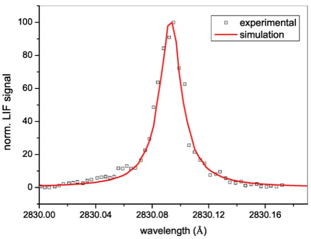
• the Q1(1) at2819.13Å and the Q2(3) at2829.37Å for measurements of OH density;

(46)

32 CHAPTER 3. LASER INDUCED FLUORESCENCE

• the group of lines Q12(1) at 2829.21Å, Q2(1) at 2829.23Å, Q1(6) at 2829.27Å,

Q12(3) at2829.31Å and Q2(3) at2829.37Å for temperature measurements.

Figure 3.1:Laser Induced Fluorescence spectrum in a He−H2O dielectric barrier discharge, after excitation of

OH(A2Σ+, v0 = 1, N0 = 1)by scheme 1. The rotational transitions labels refer to the nascent

spectrum, which is the expected one in the absence of RET collisions.

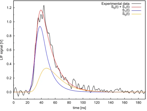
The fluorescence is captured by a broadband detection. Due to fast RET collisions, the

initial population of the rotational level N’ excited by the laser is quickly redistributed in

the whole rotational manifold towards a Boltzmann distribution at equilibrium with the gas

temperature. This can be seen in Figure 3.1, in which the observed fluorescence spectrum

shows a thermalised rotational distribution, in contrast with the nascent spectrum (i.e. in the

absence of RET collisions) that contains only transitions coming from the N’=1 pumped

level.

Another clear feature of the spectrum shown in Figure 3.1 is the presence of the (0,0)

vibro-electronic band, in spite of the fact that only the (1,1) band has been pumped by the

(47)

3.3. LIF EXPERIMENTAL SET-UP 33

Figure 3.2:Schematic representation of a LIF experiment; the sampled volume is defined by interception

between the laser beam (that excite the OH molecules) and the collection lens cone of acceptance.

presents the basic arrangement of our LIF experiment. The laser beam is injected into the

target either directly or focalised (as in Figure 3.2). The fluorescence signal is observed

in the scattering arrangement, in which the signal is collected from a different direction

from the laser beam [42]. Collecting the LIF signal perpendicular to the laser beam is the

arrangement of choice in order to prevent stray light caused from scattering at optical

sur-faces. Thanks to this configuration, the spatial resolution of the measurement is very high.

The sampled volume is defined by the intersection of the laser beam (whose diameter is

2w0) and the collection lens acceptance cone (defined by the solid angleΩand the distance

between the sampled volume and the lens).

3.3

LIF Experimental Set-up

The LIF experimental set-up is composed of three main parts: the laser light generation

and manipulation apparatus, the collection and detection of fluorescence signal system, and

the PC-based control system.

3.3.1 Laser light generation and manipulation

The quality (in terms of beam profile) of the generated laser beam, energy and

(48)

measure-34 CHAPTER 3. LASER INDUCED FLUORESCENCE

ments. We modified the laser-light source to have a more stable source in terms of

wave-length and more reliable wavewave-length scanning. In addition we spatially filtered the laser

beam, so that hot spots and excessive long tails are removed from the laser beam spatial

profile.

Laser source

Figure 3.3:UV-laser source setup: Nd:YAG: Q-switched laser, SHG: frequency doubling crystals, Trg. PD:

interferometer sample and hold circuit trigger source photodiode, Int PD: interferometer signal

photodiode, CCD: camera to record the etalon fringe pattern

The laser source set-up is shown in Figure 3.3. It is composed of a dye laser (TDL50,

Quantel) pumped by a Q-switched Nd:YAG laser (YG580, Quantel). The Nd:YAG laser

works with a repetition rate of10Hz, generating a1064nm pulse. Frequency doubling is

achieved by passing the beam through a second harmonic generator (type II KDP crystal).

The obtained532nm average power is360mJ pulse−1and serves to pump the dye laser. A mixture of methanol and Rhodamine 590 chloride (Exciton,89mg l−1, tuning range552− 584nm ) flows in the dye laser oscillator and pre-amplifier dye cells. Only methanol flows in

the second capillary dye cell, because the energy of the beam generated by the pre-amplifier

(49)

3.3. LIF EXPERIMENTAL SET-UP 35

2810Å, after fundamental separation, is around0.53mJ pulse−1. UV-beam separation from the fundamental is achieved using a wavelength filter composed of two CaF₂ Pellin-Broca

prisms and a beam stopper in the middle.

In order to prevent dye laser wavelength fluctuations during fixed wavelength

opera-tions, and to perform more accurate scans (avoiding the use of the dye laser motors to move

the tuning mirror), we modified the moving system of the tuning mirror of the laser cavity.

A representation of the Quantel TDL50 sine drive mechanism is presented in Figure 3.4.

Figure 3.4:Comparison between the original sine drive mechanism of the dye laser tuning mirror (on the left),

and the modified one (on the right)

On the left it is shown the original one, where the sine bar rotating arm (B), that is

con-nected through the rotational axis (A) to the tuning mirror, is moved by a liner translation

stage. The translation stage and the nut (C) are moved by the lead screw (D) rotation. On

the right the modified mechanism is presented. An adjustment screw (G) and a

piezoelec-tric actuator (E) (Thorlabs AE0505D16, housed in a holder (F) connected to the sine bar

rotational arm) are placed between the sine bar rotating arm and the translation stage. The

measured conversion factor between the linear translation stage displacement and the

wave-length variation isξ = 5×103pm mm−1 in the original mechanism. In this configuration the distance between the centre of the rotational axis (A) and the point of contact of the

linear translation stage with the sine bar translation arm is L = 85mm. In the new

con-figuration the distance between the centre of the rotational axis (A) and the centre of the

piezoelectric actuator holder (F) isl= 35mm. In both cases the angle between the vertical

(50)

36 CHAPTER 3. LASER INDUCED FLUORESCENCE

The nominal piezoelectric actuator displacement at the maximum working voltage (100V)

is∆l= 12(2)µm, so the maximum wavelength displacement is given by:

∆υ=ξL l

∆l

cos(α) = 16(3)×10pm.

In this way, it is possible to perform wavelength scans by using only the piezoelectric

ac-tuator (for intervals smaller than∆υ), or to use the original system based on DC motors

controlled by the PC (see Chapter 3.3.4). Moving the tuning mirror with the piezoelectric

actuator has the disadvantage that the dye laser control unit cannot read the actual

wave-length. The laser control unit calculates the wavelength by using an optical encoder

connec-ted directly to the lead screw and moved by the DC motors.

During fixed wavelength laser operations, when the laser needs to be tuned to a

mo-lecular transition for a long time, it is crucial to avoid changes of the output wavelength of

the dye laser. Temperature drifts and mechanical relaxations of the mechanism that controls

the tuning mirror of laser cavity cause variations of the beam wavelength in the order of

10−20pm h−1. To fix this problem, we implemented a feedback mechanism for the dye laser based on a etalon and a CCD (Figure 3.3). A fraction of the laser beam is sampled

be-fore the Pellin-Broca prisms by using a wedge quartz window. The sampled beam is sent to

af = 40mm BK7 lens. The etalon (F SR= 10GHz, broadband) is placed behind the lens

focal point, in order to have a divergent beam incident on it. A50−200mm manual

cam-era lens (Tamron) coupled with a grey-scale CCD (DMK 41AU02.AS, Imaging Source) are

used to record the interference fringes. The exposure time of the CCD is set to300ms, shots

are recorded and analysed with a program written in LabVIEW. The stabilisation program

of the laser records the etalon picture, creates the image histogram, along a direction defined

by the user, which intercepts the more intense interference fringes and performs the peak

detection. Positions (in pixel) of two fringes are recorded to track the wavelength (absolute

position) and to calculate the conversion factor between the etalon free spectral range (FSR)

and the camera pixels (relative position). The change in the absolute position of one of the

two fringes is used to generate a signal that is converted in the voltage of the

piezoelec-tric actuator to correct the dye laser output wavelength. The laser beam is stabilised within

0.1pm h−1around the desired wavelength.

(51)

3.3. LIF EXPERIMENTAL SET-UP 37

necessary to measure the change in wavelength. For this purpose, a small fraction of the

dye beam is sampled by a quartz wedge window and sent to a low-finesse Fabry–Pérot

interferometer made by a1/200thick200-diameter BK7 window. The interferometer FSR is

given by:

F SR= λ

2

2nlcosϑ = 8.1pm

wheren= 1.51794is the BK7 refractive index atλ= 562nm,ϑ= 0◦is the angle between

the incident beam and the window, and l = 12.84mm the window thickness. An iris is

placed in between the two windows to align the etalon. Interference fringes reflected by

the interferometer are detected for each laser shot, by using a photodiode placed behind the

wedge window. The other part is sent to another photodiode that serves as trigger source for

the sample-and-hold circuit that carries out the interferometer readout.

3.3.2 Beam Optics

Figure 3.5:UV-beam optics set-up schematic representation. Var. Atten.: optical variable attenuator; trg PD:

oscilloscope acquisition trigger source; PM1: low energy (< 4µJ pulse−1) power monitor; PM2:

high energy (>4µJ pulse−1_{) power monitor.}

The UV laser beam is injected in a separate breadboard, where it is manipulated to hit

(52)

38 CHAPTER 3. LASER INDUCED FLUORESCENCE

right angle prisms that correct propagation, height, and direction of the beam. To change

the power injected into the target, we developed a variable optical attenuator based on

Fres-nel reflection, suitable for applications where a high-peak power is involved [61]. A further

requirement is that the optical variable attenuator does not significantly alter the beam

pro-file, position and direction. A detailed description of the device design and performances is

reported in Appendix A.1.

The attenuated beam passes through a spatial filter composed of twof = 100mm

bi-convex UVFS lenses, and a pinhole to filter the beam noise. The pinhole cuts the wings

of the spatial Fourier-mode spectrum of the incoming beam. Beam imperfections, due to

laser generation, frequency doubling and optics quality, cause structures in the beam with

higher spatial modes that are cut off by the pin-hole [62]. The estimated beam waist is

23(3)µm in the focal plane of the spatial filter. We chose a∅50µm high-power precision

pinhole (P50C, Thorlabs) coupled with a precision positioning system (M-461-XYZ-M,

Newport). A wedge UVFS window is placed after the spatial filter to sample a fraction of

the incident beam, which is then used to generate the acquisition trigger signal. A 12V

reverse biased broad-band UV SiC photodiode (SG01M, Sglux), coupled with a diffuser,

collects the trigger beam and records the time profile of the laser. The filtered laser beam is

then injected in the target area, either directly (with a2mm beam diameter) or focalised by

af = 250mm UVFS plano-convex lens (expected beam diameter is0.2mm).

In order to avoid back reflection of the UV-beam into the target area, an aluminium

mirror (working at45◦) directs the beam towards the detection system. For low energies

(E <4µJ pulse−1), a single-channel silicon-based thermopile (DX-0576, Dexter research center) is used. The thermopile output voltage is amplified by a non-inverting amplifier with

gainG= 500, and the peak voltage of the signal is acquired by using a digital multimeter

(34410A, Agilent). The pulse energy is inferred from the peak voltage, which in turn is

proportional to the energy deposited on the detector (see Appendix A.2.1 for a detailed

de-scription). In the case of higher energies (E >4µJ pulse−1), the moving mirror is removed and the UV-beam energy is measured by using a pyroelectric detector (P1-13, Molectron),

amplified by a high speed non-inverting amplifier, and then digitising by using an

(53)

3.3. LIF EXPERIMENTAL SET-UP 39

allows us to record the amplifier output simultaneously to the signal of the photomultiplier

tube. I describe two devices in Appendix A.2.

3.3.3 Fluorescence detectors

The laser induced fluorescence is emitted isotropically from the target [63]. The

col-lection of the fluorescence emitted perpendicular with respect to the laser beam is the

ar-rangement of choice in order to minimise the possibility of collecting scattered laser light.

A schematic representation of the fluorescence detection optics is shown in Figure 3.6. The

Figure 3.6:Schematic representation of the laser induced fluorescence detector arrangement. PMT: gated

pho-tomultiplier tube for time-resolved measurement; ICCD: multi-channel plate plus charge coupled

device.

fluorescence signal emitted is collected by a f = 200mm ∅ = 100 UVFS plano-convex

lens. Two ∅ = 200 enhanced aluminium mirrors (omitted in figure) are used to direct the

light to the monochromator entrance slit. Af = 75mm UVFS plano-convex matches the

incoming beam to the f-number of the monochromator. A set of four neutral density

fil-ters (NDUV01B,NDUV03B,NDUV06B and NDUV510B, Thorlabs) is placed in front of

the input slit to change the incoming light intensity. A Shamrock 303i300mm focal length

monochromator, equipped wit

Density measurement of OH radicals in non-thermal plasmas by laser induced fluorescence and time-resolved absorption spectroscopy

NIVERSITY OF

DEPARTMENT OFPHYSICS

ATTEO

IN CANDIDATURE FOR THE DEGREE OF

PHILOSOPHIAE

TUTOR: PROF. PAOLOTOSI

Members of the doctoral thesis

Acknowledgements

Contents

Chapter 1

2 CHAPTER 1. INTRODUCTION

1.1. APPLICATIONS OF AP-NTPS 3

4 CHAPTER 1. INTRODUCTION

Optical spectroscopy diagnostics of discharges at

Chapter 2

6 CHAPTER 2. TR-BBAS

Broad band absorption spectroscopy: principles and

2.1. BBAS: PRINCIPLES AND APPLICATION TO OH 7

8 CHAPTER 2. TR-BBAS

Time-resolved broad-band absorption spectroscopy

2.2. TR-BBAS SET-UP 9

10 CHAPTER 2. TR-BBAS

2.2. TR-BBAS SET-UP 11

2.2. TR-BBAS SET-UP 13

14 CHAPTER 2. TR-BBAS

2.3. MEASUREMENT STRATEGY 15

Measurement strategy

16 CHAPTER 2. TR-BBAS

2.3. MEASUREMENT STRATEGY 17

18 CHAPTER 2. TR-BBAS 0.00 0.25 0.50 0.75 1.00

2.3. MEASUREMENT STRATEGY 19

20 CHAPTER 2. TR-BBAS

2.3. MEASUREMENT STRATEGY 21

22 CHAPTER 2. TR-BBAS

2.3. MEASUREMENT STRATEGY 23

24 CHAPTER 2. TR-BBAS

2.3. MEASUREMENT STRATEGY 25

26 CHAPTER 2. TR-BBAS

2.3. MEASUREMENT STRATEGY 27

Chapter 3

30 CHAPTER 3. LASER INDUCED FLUORESCENCE

Literature overview

3.2. SPECTROSCOPIC SCHEME 31

Spectroscopic scheme

32 CHAPTER 3. LASER INDUCED FLUORESCENCE

3.3. LIF EXPERIMENTAL SET-UP 33

LIF Experimental Set-up

3.3. LIF EXPERIMENTAL SET-UP 35

36 CHAPTER 3. LASER INDUCED FLUORESCENCE

3.3. LIF EXPERIMENTAL SET-UP 37

38 CHAPTER 3. LASER INDUCED FLUORESCENCE

3.3. LIF EXPERIMENTAL SET-UP 39