Modeling and Control of Three-Phase Gravity Separators in Oil
Production Facilities
Atalla F. Sayda and James H. Taylor
Abstract— Oil production facilities exhibit complex and challenging dynamic behavior. A dynamic mathematical mod-eling study was done to address the tasks of design, control and optimization of such facilities. The focus of this paper is on the three-phase separator, where each phase’s dynamics are modeled. The hydrodynamics of liquid-liquid separation are modeled based on the American Petroleum Institute design criteria. Given some simplifying assumptions, the oil and gas phases’ dynamic behaviors are modeled assuming vapor-liquid phase equilibrium at the oil surface. In order to validate the developed mathematical model, an oil production facility simulation was designed and implemented based on such models. The simulation model consists of a two-phase separator followed by a three-phase separator. An upset in the oil component of the incoming oil-well stream is introduced to analyze its effect of the different process variables and produced oil quality. The simulation results demonstrate the sophistication of the model in spite of its simplicity.
I. INTRODUCTION
The function of an oil production facility is to separate the oil well stream into three components or “phases” (oil, gas, and water), and process these phases into some marketable products or dispose of them in an environmentally accept-able manner. In mechanical devices called “separators”, gas is flashed from the liquids and “free water” is separated from the oil. These steps remove enough light hydrocarbons to produce a stable crude oil with the volatility (i.e., vapor pressure) to meet sales criteria. Separators are classified as “two-phase” if they separate gas from the total liquid stream and “three-phase” if they also separate the liquid stream into its crude oil and water components. The gas that is separated is compressed and treated for sales [1]. Modeling such facilities has become very crucial for controller design, fault detection and isolation, process optimization, and dynamic simulation. In this paper, we focus on three-phase gravity separators as they form the main processes in the upstream petroleum industry, and have a significant economic impact on produced oil quality.
Three-phase separators have rich and complex dynam-ics, which span from hydrodynamics to thermodynamics and conservation laws. Many modeling techniques and approaches have been used to model three-phase separators. As far as the thermodynamics aspects of the separator are concerned (i.e., the oil and gas phases), many modeling approaches have been suggested in the literature. The phase equilibrium modeling approach have been used for 50 years
James H. Taylor is a professor with the Department of Electrical & Computer Engineering, University of New Brunswick, PO Box 4400, Fredericton, NB CANADA E3B [email protected]
Atalla F. Sayda is a PhD candidate with the Department of Electrical & Computer Engineering, University of New Brunswick, PO Box 4400, Fredericton, NB CANADA E3B [email protected]
and has provided satisfactory results for such equipment as flash tanks and distillation columns [2]. The basic equations in this approach are used to describe the material balances, equilibrium relations, the composition summation equa-tions, and the enthalpy equations. Nonequilibrium models have been developed to describe real physical separation processes; other modeling approaches were also considered such as the computational model, the collocation model, and the bubble residence contact time model [3].
Historically, the hydrodynamics of the separator’s aque-ous part have been modeled using complex mathematical-numerical models, which describe the coalescence and settling of oil droplets in oil-water dispersions. Such models take into account separator dimensions, flow rates, fluid physical properties, fluid quality and drop size distribution. The output of these models is the quality of the output oil [4]. Other models, which describe the kinetics of low Reynolds number coalescence of oil droplets in water-oil dispersions, have been developed to give the volumes of separated continuous-phase and coalesced drops [5]. A computational fluid dynamic (CFD) model was developed to model the hydrodynamics of a three-phase separator, based on the time averaging of Navier-stokes equations for three phases; it takes into consideration the non-ideal flow due to inlet /outlets and internal equipment for separation enhancement [6]. The “alternative path model approach”, which exploits the residence time distribution (RTD) of both oil and aqueous phases in three-phase separators, was de-veloped to give a quantitative description of hydrodynamics and mixing in the aqueous phase [7]. Powers [8] extended the American Petroleum Institute (API) gravity separator design criteria to design free-water knockout vessels for better capacity and performance. Powers showed that the API design criteria can handle nonideal flow by performing practical RTD experiments.
II. THREE-PHASE GRAVITY SEPARATION PROCESS DESCRIPTION
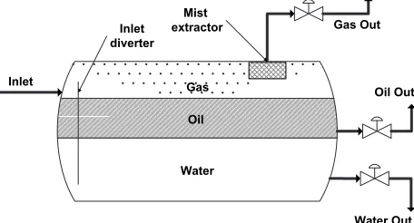
Three-phase separators are designed to separate and re-move the free water from the mixture of crude oil and water. Figure 1 is a schematic of a three phase horizontal separator. The fluid enters the separator and hits an inlet diverter. This sudden change in momentum does the initial gross separation of liquid and vapor. In most designs, the inlet diverter contains a downcomer that directs the liquid flow below the oil /water interface. This forces the inlet mixture of oil and water to mix with the water continuous phase (i.e., aqueous phase) in the bottom of the vessel and rise to the oil /water interface. This process is called “water-washing”; it promotes the coalescence of water droplets which are entrained in the oil continuous phase. The inlet diverter assures that little gas is carried with the liquid and assures that the liquid is not injected above the gas /oil or oil /water interface, which would mix the liquid retained in the vessel and make control of the oil /water interface difficult.
Some of the gas flows over the inlet diverter and then horizontally through the gravity settling section above the liquid. As the gas flows through this section, small drops of liquid that were entrained in the gas and not separated by the inlet diverter are separated out by gravity and fall to the gas-liquid interface. Some of the drops are of such a small diameter that they are not easily separated in the gravity settling section. Before the gas leaves the vessel it passes through a coalescing section or mist extractor to coalesce and remove them before the gas leaves the vessel.
Fig. 1: Three phase horizontal separator schematic.
III. THREE PHASE GRAVITY SEPARATOR
MATHEMATICAL MODELING
When the hydrocarbon fluid stream enters a three-phase separator, two distinctive phenomena take place. The first phenomenon is fluid dynamic, which is characterized by the gravity separation of oil and water droplets entrained in the aqueous and the oil phases respectively, the gravity separation of gas bubbles entrained in the stream, and the gravity separation of liquid droplets which are dispersed in the gas phase. The second phenomenon is thermodynamic, in the sense that some light hydrocarbons and gas solution flash out the oil phase and reach a state of equilibrium due to the pressure drop in the separator. Due to the complexity
of such phenomena, we are going to focus on the hydro-dynamic separation of oil droplets entrained in the aqueous phase and the thermodynamic separation of gas and light hydrocarbons from the oil phase. This decision is justified by the fact that the water washing process minimizes the water entrained in the oil phase. Furthermore, preceding gravity separation processes minimize the amounts of gas entrained in the main stream.
Figure 2 illustrates the simplified separation process, where an oil-well fluid with molar flow Fin and gas, oil, and water molar fractions Zg, Zo, Zw respectively enters the separator. The hydrocarbon component of the fluid separates into two parts; the first stream Fh1 separates by
gravity and enters the oil phase, and the second streamFh2
stays in the aqueous phase due to incomplete separation. The liquid discharge from the aqueous phase FWout is a combination of the dumped water stream FW plus the unseparated hydrocarbon stream Fh2. The gas component
in the separated hydrocarbon stream, which enters the oil phase, separates into two parts; the first gas stream Fg1
flashes out of the oil phase due to the pressure drop in the separator, and the second gas streamFg2 stays dissolved in
the oil phase. The oil discharge Foout from the separator contains the oil component of the separated hydrocarbon Fo and the dissolved gas componentFg2. The flashed gas
Fgout flows out of the separator for further processing.
Fig. 2: Main separated component streams in three-phase gravity separator
We model the dynamics of each phase of the separa-tor in the subsequent sections, to simplify the modeling process. Additionally, some simplifying assumptions have to be made. The separation processes are assumed to be isothermal in all phases of the separator at100oF. We also assume that the flow pattern in the liquid phases is plug flow, especially in the aqueous phase. Furthermore, the oil droplets in the aqueous phase have a uniform droplet size distribution with a diameter of dm= 500 micron. The oil droplets’ rising velocities are assumed to obey Stokes’ law. We model the equilibrium thermodynamics phenomenon under the assumption that Raoult’s law is valid. We assume that only one light hydrocarbon gas flashes out the oil phase into the gas phase, namely methane. Methane in the vapor phase is also assumed to be an ideal gas (i.e., the ideal gas law applies). Finally, there is liquid-vapor equilibrium at the oil surface and liquid-liquid equilibrium at the water-oil interface.
A. The aqueous phase
simplifying assumptions. The API specification permits hydrocarbon droplets (i.e., oil and dissolved light gas) of design diameter to rise from the bottom of the separator to the surface during the water retention period, as illustrated in figure 3. A hydrocarbon droplet located on the cylinder bottom has the greatest distance to traverse to the oil-water interface. Therefore, modeling the oil separation hydrody-namics based on removal of this droplet would ensure re-moval of all others of the same or larger diameter. Given the simplifying assumptions, the traversing hydrocarbon droplet on its path to the oil-water interface is subjected to a vertical rising velocity componentvv governed by Stokes’ law, and a horizontal velocity component vh governed by the plug flow pattern of the aqueous phase. The vertical velocity component is estimated from Stokes’ law by equation (1):
vv= 1.7886×10⁻⁶(SGh−SGw)d2m
µw (1)
where SGh, SGw are the specific gravities of the hydro-carbon droplets and water, respectively, dm is the droplet diameter in microns, and µw is the water viscosity in CP at 100oF. The horizontal velocity component is estimated from the aqueous phase retention as vh =L / τ, where L is the length of the separator and τ =Vwat/ Fwat is the retention time of the aqueous phase;Vwatis the volume of the aqueous phase, andFwatis the water outflow. The level of the oil-water interface h is determined from equations (2):
Ac = Vwat/L
= R2θ −0.5R2sin(2θ)
h = R(1−cos(θ)) (2)
whereAc is the cross-sectional area of the aqueous phase, R is the separator radius andθ is the angle which defines the circle sector of the cross sectional area Ac. The angle Φof the longest droplet path to the oil-water interface can be estimated from equation (3):
Φ = tan−1vv
vh (3)
Fig. 3: Oil separation hydrodynamics under normal operation conditions
The design parameters {Ac, h, θ,Φ} of the aqueous phase will take their nominal values under normal operating conditions of the three-phase separator, i.e., for the nominal value ofFwatwhich leads to complete separation, as shown
in figure 3. However, our model must also be valid for off-nominal values. This is complicated at higher flow values, since we can no longer achieve complete separation. Let us assume that the water outflow Fwat has increased by a value of∆Fwat due to a corresponding increase in inflow. This will result in an increase in vh to vh+ ∆vh and an angle change of the longest path of a traversing hydrocarbon droplet fromΦtoΦ1<Φ. Figure 4 illustrates the concept
of virtually extending the tank so that complete separation would be achieved at L1 = L+ ∆L, although this is
fictional. Assuming that the design parameters {Ac, h, θ}
remain the same, as shown in figure 4, we have:
Φ1 = tan−1(vv+δvv)
vh (4)
L1 = hcot(Φ1)
We have to make a simplifying assumption in order to estimate the volume fraction of unseparated hydrocarbon,ε. As shown in figure 5 (top), we assume that the unseparated oil droplets in the aqueous phase form a “tail” extending into the virtual separator extension, as also shown by dashed lines in figure 5 (bottom, labelled S3) that undergoes turbulent flow and exits with the water. The accuracy of this assumption is, of course, dependent upon the geometry of the tank and structure of the water and oil outlets.
Fig. 4: Oil separation hydrodynamics under high water outflow condition
Under this assumption, region S3 in the bottom fig-ure represents the volume of the unseparated hydrocarbon fluid VS3. It can be seen from figure 5 that region S3
is the difference between the hydrocarbon fluid volume in the virtual separator (represented by region S1), VS1
and the hydrocarbon fluid volume in the actual separator, VS2 (represented by region S2). The volume VS1 can be
calculated as the difference between the volume of the cylindrical segment defined by the parameters {h, L1, θ}
and the cylindrical wedge parameterized by {h, L1,Φ1},
as in equation (5):
VS1=R2L1{θ−0.5 sin(2θ)−
3 sinθ−3θcosθ−sin3θ
3(1−cosθ) } (5) Furthermore, again referring to figure 5, the volumeVS2
can be estimated as the difference between the volume of the cylindrical segment parameterized by{h, L, θ}and the cylindrical wedge parameterized by{h1, θ1, L,Φ1}, as in
VS2=R2L{θ−0.5 sin(2θ)−3 sinθ1−3θ1cosθ1−sin 3θ
1
3(1−cosθ1) }
(6) where the virtual oil-water interface h1 and angle θ1 are
defined by equations (7):
h1 = Ltan(Φ1)
θ1 = cos−1(1−h1
R) (7)
Consequently, we can estimate the unseparated hydrocar-bon fluid volume fractionεfrom equation (8):
ε=
½
1−VS2
VS1 , L1> L
0 else (8)
Fig. 5: Unseparated hydrocarbon fluid volume under high water outflow condition
Having estimated the unseparated hydrocarbon fluid vol-ume fractionε, we can calculate the separated and unsepa-rated volumetric flow components of the hydrocarbon fluid Fh1v, Fh2v respectively. Finally we can write the dynamic material balance of the aqueous phase by using equations (9), after we convert the molar flows to volumetric flows:
Fh1v =
ε(Zg+Zo)FinM wh 62.43SGh
Fh2v =
(1−ε)(Zg+Zo)FinM wh 62.43SGh
FWout =
ZwFinM ww 62.43SGw +Fh2v
dVwat
dt =
FinM win
62.43SGin−FWout−Fh1v (9)
where {M wh, M ww, M win} are the hydrocarbon,
water, and incoming mixture molecular weights;
{SGh, SGw, SGin} are the hydrocarbon, water, and incoming mixture specific gravities; Vwat is the aqueous
phase volume; andFWout is the water discharge volumetric outflow.
B. The oil phase
In order to model the thermodynamic phenomenon in the oil phase, we first do the flash calculations to estimate the amounts of gas which will flash out of solution. Since we assumed that ideal phase equilibrium state is valid, then by applying Raoult’s law we can tell how much methane will stay entrained in the oil phase. Raoult’s law relates the vapor pressure of components to the composition of the solution. This can be formulated mathematically as yiP = xiPvi whereyiis the mole fraction of the component i in the vapor phase,xi is the mole fraction of component i in the liquid phase,P is the total pressure of the vapor phase (i.e., the separator working pressure), andPvi is the vapor pressure of componenti[9], [10].
Since we have only one flashing light hydrocarbon (i.e., methane), this implies that the mole fraction of methane in the vapor phase is y = 1, and that the mole fraction of methane entrained in the liquid phase is x = P/Pv. Given the composition {Zg1, Zo1} of the separated
hy-drocarbon stream Fh1, we can estimate the amounts of
flashing methaneFg1and dissolved methane in the oil phase
Fg2. The oil discharge flow Foout can also be estimated along with its average molecular weight M wo1 and its
specific gravitySGo1. The complete dynamic model of the
oil phase, which is given by equations (10), can be then formulated by taking the material balance:
Fg1 = (1−x)Zg1Fh1
Fg2 = xZg1Fh1
Foout = Fo+Fg2
dNoil
dt = Fh1−Fg1−Foout
M wo1 = xM wg+ (1−x)M wo
SGo1 = xM wgNoilxM w + (1−x)M woNoil
gNoil
SGg +
(1−x)M woNoil
SGo
(10)
whereNoil is the number of liquid moles in the oil phase; Fo is the molar oil component in the oil discharge flow Foout;{M wg, M wo}are the gas and oil molecular weights; and{SGg, SGo} are the gas and oil specific gravities.
C. The gas phase
Given the ideal gas law assumption, the gas phase of the separator is modeled by taking the material balance. We can estimate the gas pressureP by applying the ideal gas law, as described by equations (11):
dNgas
dt = Fg1−Fgout
Voil = M wo1Noil 62.43SGo1
Vgas = Vsep−Vwat−Voil
P = NgasRT
where Ngas is the number of gas moles in the gas phase; Fgout is the gas molar outflow from the separator;
{Voil, Vgas, Vsep} are the volumes of the oil phase, gas phase, and separator respectively; R is the universal gas constant; andT is the absolute separator temperature.
IV. SEPARATOR MODEL VALIDATION
Having obtained the dynamic model of the three-phase gravity separator, we design a simulation model which emulates an oil production facility to validate the model behavior under several scenarios. The simulation model basically consists of three processes, as depicted in figure 6. The first is a two-phase separator in which hydrocarbon fluids from oil wells are separated into two phases (gas, oil + water) to remove as much light hydrocarbon gases as possible. The separator is 15 ft long and has a diameter of 5 ft. The two-phase separator model was developed based on the models of the oil and gas phases of the three-phase sep-arator. That is, we have modeled only the thermodynamic phenomenon of gas flashing out the liquid phase. The liquid produced is then pumped to the three-phase separator (i.e., the second process), where water and solids are separated from oil. The oil produced is then pumped out and sold to refineries and petrochemical plants if it meets the required specifications. The three-phase separator has length of 8.6 ft and a diameter of 4.8 ft. Flashed light and medium gases from the separation processes are sent to a gas scrubber where medium hydrocarbon and other liquid remnants are separated from gas and sent back for further treatment. Produced gas is then compressed by a compressor (i.e., the third process) and pumped out for sales. The third process model was not included in the simulation model for the sake of simplicity.
The two separation processes in the simulation model are controlled to maintain the operating point at its nominal value, and to minimize the effect of disturbances on the produced oil quality. As shown in figure 6, the first separa-tion process is controlled by two PI controller loops. In the first loop, the liquid level is maintained by manipulating the liquid outflow valve. The second loop controls the pressure inside the two-phase separator by manipulating the amount of gas discharge. The second separation process has three PI controller loops. An interface level PI controller maintains the height of the oil /water interface by manipulating the water dump valve, while the oil level is controlled by the second PI controller through the oil discharge valve. The vessel pressure is maintained constant by the third PI loop.
V. SIMULATION RESULTS
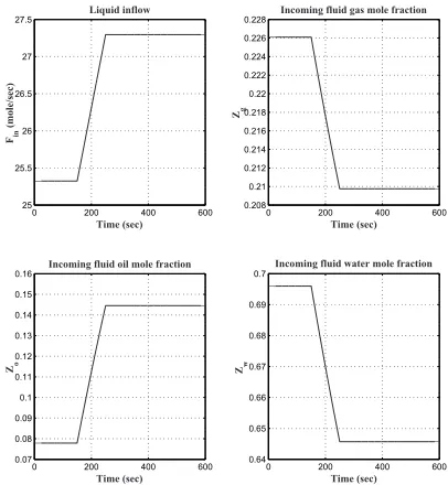
The two-phase separator process operates at a liquid phase volume of 146 ft3 and working pressure of 625 PSI. In contrast, the three-phase separator operates at water phase volume of 77.5 ft3, oil phase volume of 46.5 ft3, and working pressure of 200 PSI. The working temperatures of the two separation processes are 100oF. The facility processes hydrocarbon streams of 25.23 moles /sec from oil wells under pressure of 1900 PSI. The incoming stream has mole fractions of 22.61% gas, 7.79% oil, and 69.6%
water. In order to demonstrate the dynamic behavior of the separators, the oil content of the incoming stream has been increased linearly by 2 moles /sec between the time instants t1 = 150 sec and t2 = 250 sec of the simulation time.
Figure 7 portrays this change in the incoming stream flow and in its molar composition; the oil mole fraction increased while the water and gas mole fractions decreased.
Fig. 7: Incoming hydrocarbon fluid and its molar composition
The ramp increase in the oil component of the incoming stream caused the liquid volume and gas pressure in the two-phase separator to peak to 167 ft3 and 630 PSI respec-tively, as shown in figure 8. The two PI control loops of the two-phase separator intervened to correct such operating point errors by manipulating the liquid and gas outflows. This operating point disturbance took approximately 300 sec to be totally rejected by the separator control system. Figure 8 also reveals the difference between the dynamics of the two phases of the separator. The liquid phase has slower dynamics than the gas phase dynamics, i.e., the pressure changes faster than the liquid volume. It is interesting to no-tice that the liquid molar outflow increased by 2 moles /sec, which is the same applied change in the incoming stream. This reflects on the quality of the liquid produced in terms of its specific gravity, which increased from 31.7o API to
35.3o API. The quality change can be verified by plotting the molar composition of the liquids produced, as shown in figure 9. The oil mole fraction of the produced liquid increased, while the mole fractions of dissolved gas and water decreased.
Group Separator
Oil Treator Gas Scrubber
Gas compressor
Oil well
Water treatment Water
CV1 CV5
CV3 CV2
CV4
Water
Oil & water mix
Water Oil
CV7
P
PT1
P
PT2
P
PT3
I-8
I-10
I-11
I-1
3
I-14
I-15
I-16
I-1
7
I-18
CV6
I-1
9
To water treatment
Oil sales Gas sales
Disposal CV8
P
PT4
I-22
Gas
Gas
Gas
Pipe line
Signal line LCL : Level control loop
LCL 1
LCL 2 LCL 3
LCL 4
PCL : Pressure control loop PCL 1
PCL 2
PCL 3
PCL 4
FT1
FT2 FT6 FT3
FT4
FT5
FT7 FT8
Motor LT1
LT3
LT2 LT4
FT : Flow transmitter PT : Pressure transmitter LT : Level transmitter CV : Control valve
N1
Fig. 6: The oil production facility schematic diagram
!
"
" ! #
Fig. 8: Two-phase separator process variables change during the incoming stream upset
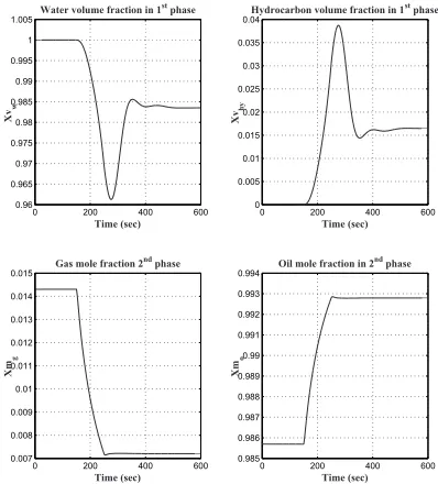
gas phase dynamics compared to the two liquid phases), the upsets are rejected in approximately300seconds. However, two main events should be noticed; the first event is the slight increase in the water discharge molar flow. This can be attributed to inefficiency in the gravity separation hydrodynamics, which implies that some oil could not be separated and was discharged with water. We can verify this event by plotting the volumetric composition of the dumped water (“1st phase”), as shown by the top plots in figure 11. The dumped water volumetric composition reveals that some amounts of unseparated oil has been lost.
Fig. 9: Two-phase separator liquid discharge molar composition
gas mole fraction decreased. This simulation study demon-strated the sophistication of the three-phase separator model, in spite of its simplicity. Not only did the model address the quantity dynamics of separator process variables, but the quality of the produced oil and water also.
Fig. 10: Three-phase separator process variables change during the incoming stream upset
Fig. 11: Three-phase separator produced water and oil compositions
VI. CONCLUSIONS
A dynamic mathematical model was developed for an oil production facility. The focus of this study was on the three-phase separator, where each phase’s dynamics were modeled. The hydrodynamics of liquid-liquid separation were modeled based on the API design criteria, which was extended to address the process dynamics in addition
to its statics. The oil and gas phases’ dynamic behaviors were modeled assuming vapor-liquid phase thermodynamic equilibrium at the oil surface.
An oil production facility simulation was designed based on such model, in order to test and validate the developed mathematical model. The simulation model consisted of a two-phase separator followed by a three-phase model. The separation processes were controlled by PI control loops to maintain the operating point at its nominal value. An upset in the oil component of the incoming oil-well stream was introduced to analyze its effect of the different process variables and produced oil quality. The simulation results proved the sophistication of the model in spite of its simplicity. Furthermore, this study demonstrated the challenging task of modeling and controlling oil and gas production facilities, and that more work has to be done to develop higher fidelity models.
VII. ACKNOWLEDGEMENT
This project is supported by the Atlantic Canada Op-portunities Agency (ACOA) under the Atlantic Innovation Fund (AIF) program. The authors gratefully acknowledge that support and the collaboration of Cape Breton University (CBU), the National Research Council (NRC) of Canada, and the College of the North Atlantic (CNA). The first-named author also acknowledges the support of the Natural Sciences and Engineering Research Council of Canada (NSERC) for funding this research.
REFERENCES
[1] K. Arnold and M. Stewart, Surface Production Operation: Design
of Oil-Handling Systems and Facilities, 2nd ed. Woburn, MA: Butterworth-Heinemann, 1999, vol. 1.
[2] R. Taylor and A. Lucia, “Modeling and analysis of multicomponent separation processes,” Separation Systems and Design, pp. 19–28, 1995.
[3] M. M. Dionne, “The dynamic simulation of a three phase separator,” Master’s thesis, University of Calgary, 1998.
[4] B. Hafskjold, H. K. Celius, and O. M. Aamo, “A new mathematical model for oil/water separation in pipes and tanks,” SPE Production
& Facilities, vol. 14, no. 1, pp. 30–36, February 1999.
[5] S. A. K. Jeelani, R. Hosig, and E. J. Windhab, “Kinetics of low reynolds number creaming and coalescence in droplet dispersions,”
AIChE Journal, vol. 51, no. 1, pp. 149–161, January 2005.
[6] A. Hallanger, F. Soenstaboe, and T. Knutsen, “A simulation model for three-phase gravity separators,” in Proceedings of SPE Annual
Technical Conference and Exhibition. Denver, Colorado: SPE, October 1996, pp. 695–706.
[7] M. J. H. Simmons, E. Komonibo, B. J. Azzopardi, and D. R. Dick, “Residence time distribution and flow behavior within primary crude oil-water separators treating well-head fluids,” Chemical Engineering
Research & Design, vol. 82, no. A10, pp. 1383–1390, October 2004.
[8] M. L. Powers, “Analysis of gravity separation in freewater knock-outs,” SPE Production Engineering, vol. 5, no. 1, pp. 52–58, February 1990.
[9] R. G. E. Franks, Modeling and Simulation in Chemical Engineering. Wiley, 1972.
[10] C. D. Holland, Fundamentals and Modeling of Separation Processes: