Мodeling of the Sea Upper Layer Ecosystem Fields by the Adaptive Balance of Causes Method

Мodeling of the Sea Upper Layer Ecosystem Fields

by the Adaptive Balance of Causes Method

I.Е. Тimchenko, I.P. Lazarchuk, I.K. Ivashchenko, E.M. Igumnova

Marine Hydrophysical Institute, Russian Academy of Sciences, Sevastopol, Russian Federation

A method for constructing the sea upper layer ecosystem fields, based on negative feedbacks in the ecosystem model, which provide mutual adaptation of biochemical processes taking into account resource limitations and external influences, is considered. This method allows us to construct cause-and-effect dependencies between the processes in complex ecosystems using negative feedbacks be-tween the ecosystem model variables and rates of their change. It is shown that such an approach retains material balances of biochemical reactions in the ecosystem and increases sensitivity of adap-tive models to the data of observations assimilated in them.A method for assimilation of calculated data on marine environment dynamics in adaptive models of marine ecosystems consisting in simul-taneous adjustment of biochemical process values to the data of satellite observations and previously obtained assessments of marine environment advection and diffusion is proposed.The method is illu-strated by the examples of constructing the charts of phytoplankton, zooplankton, bio-resource and oxygen concentrations for the shelf regions of the north-western Вlack Sea. Satellite observation data on the sea surface temperature and chlorophyll-a concentration as well as the assessments of the sub-stance simulated advection and diffusion resulted from the hydrodynamic model are used as the ex-ternal sources of influences.The coefficients of intra-system influences in ecosystem are assessed by the data of long-term observations carried out in this area.The charts of spatial-temporal fields of biochemical processes in the upper sea layer, coordinated with the charts of horizontal currents and satellite observations of chlorophyll-a concentrations are constructed. The conclusion that the ecosys-tem adaptive models should be advisably applied for obtaining the assessments of spatial distribution of the bio-chemical substance concentrations in the sea upper layer ecosystem is drawn.

Keywords: Adaptive Balance of Causes method, marine ecosystem.

DOI: 10.22449/1573-160X-2016-1-71-87

© 2016, I.Е. Тimchenko, I.P. Lazarchuk, I.K. Ivashchenko, E.M. Igumnova © 2016, Physical Oceanography

Introduction. The studies of ecosystem fields of the sea upper layer are both of scientific and practical interest due to dynamical activity and high biological productivity of marine environment of this layer. High resolution numerical models (in which the concentrations of biological objects and chemical substances are cal-culated by partial differential equations describing diffusion and transfer of sub-stances into the sea) are usually used to construct the field charts of ecosystem bio-chemical characteristics [1]. Satellite data is assimilated by these equations and, in particular, by the adaptive statistics method [2]. Due to the possibility of satellite monitoring of certain sea upper layer characteristics, the informative results on the ecosystem fields mapping (by this method) are obtained in the works on the Black Sea operative oceanography [3].

study) are performed. At the second stage these assessments and also the satellite monitoring data are used as sources of external effect in the special ecosystem model, which has a property of local adaptation to the abovementioned assessments and satellite data. Local adaptation means an automatic adjustment of ecosystem model variables to the assimilating data. This adaptation takes place due to nega-tive feedbacks between the ecosystem model variables and change rates of these variables. This fact gives reason to call this type of ecosystem models the adaptive ones [5]. Particularly, the assimilation of simulated data on transport and diffusion in marine ecosystem adaptive model, which describes the scenarios of biochemical processes in a single point of the upper sea layer, was considered in [4].

The purpose of this study is to represent the possibilities of two-stage mapping of biochemical fields by the method of local adaptation of ecosystem model va-riables. We don’t set ourselves a task to describe in details of the biochemical processes of the upper sea layer. Therefore, the simplest scheme of cause-effect relationship, which includes the concentrations of phytoplankton, zooplankton, bio-resource and dissolved oxygen, was chosen as a conceptual model. The model, in addition to these main structural elements, includes the agents of limitation of aq-uatic organism concentration increase and abovementioned sources of external ef-fects.

General equations of ecosystem adaptive model and computational algo-rithms. Marine ecosystem adaptive modelrepresents aset of interrelated processes

}

{ui satisfying the dynamical balance condition of intersystem and external influ-ences [6]. Dynamical balance is based on the tendency of living organisms to adapt to changing environmental conditions. We call “reactions” any interactions of processes in the ecosystem, which result in changes of variable values ui in the ecosystem model. Realization of such reactions assumes the presence of all re-quired components, i.e. resources, and their volumes are always limited. We will call this limiting property of environment its “resource capacity” in relation to the ecosystem model variable, which represents the product of reaction.

Variables of ecosystem model should have nonnegative values because all the biochemical processes in ecosystems are represented by concentrations of sub-stances in the marine environment. This means that,as a result of reactions, takes place the deviation of variable values from some average values

C

_i characterizing

the stationary state of the system. Therefore, the variables u_i have variation intervals

(0;

2

C

_i

)

and their resource capacities are

2

C

_i values. It is natural to assume that the models of natural ecosystems, which are in static equilibrium with the environment, have a set of average values {C_i}as a stationary state and the changes in environment lead to the deviation from this state.

An Adaptive Balance of Causes method (ABC-method), which provides a con-struction of ecosystem model equation system possessing a property of dynamic adaptation to the varying external influences, is proposed in [5]. An adaptive sys-tem mathematical model consists of ordinary differential equations of a special form, and rates of change of their variables are related by negative feedbacks with the squares of variables (second order feedbacks).

We will represent the ecosystem reactions in the form of transformations (not necessarily linear) of resources uj into the products ui with the presence of

exter-nal influencesAi:

), , , 1 ( i n C A u a

u j i i

i j

ij

i=

∑

+ + = 

≠

(1)

where aijare the coefficients of intersystem influences. These transformations

ex-press the mass balances of substances involved in the reactions. The system of АВС-method modular equations is constructed in such a way as to satisfy the bal-ance relations (1) simultaneously for all of ui variables in a model [5]:

)] (

[

2 _{j i}

i j ij i i i i i A u a u C u r dt

du _{= − −}

_∑

₋

≠

, (2)

here ri are specific rates of ui functions change.

It follows from the system of equations (2) that its stationary solution is reached at i i j i j ij

i a u A C

u −

∑

− =

≠

(3)

and it satisfies the condition of keeping the balance of influences (1). This means that during the adaptation the variables of ecosystem model take on the values that

complement the algebraic sum of intersystem j

i j iju a

∑

≠

and external Ai influences

up to the values which are equal to the halves of 2Сi resource capacity values. Un-der the effect of external influence variables a deviation of u_i values from their stationary Сi values takes place. This results in formation of steady states of dy-namic balance of influences (1). This conclusion is confirmed by the computational experiments with the equations (2) which had been carried out in [5 – 7].

General equations of АВС-method (2) are complemented with logical condi-tions (management agents) in which the resource limitacondi-tions of reaction proceeding are taken into account. One of these limitations prevents the solutions of equations from falling outside the scope of specified process variability intervals described by the following ecosystem model:

)] ; 2 ; 2 ( ; 0 ; 0

[ i i i i i

i IF u IF u C C u

u = < > . (4)

type of these resources are minimal against other types of resources. This minimal resource type will limit a zooplankton concentration increase.

In order to consider this fact the management agents )

, , min(

arg ik k in n

i a u a u

AG  are included in the АВС-ecosystem model equations:

                − − − − =

∑

≠ i n in k ik i j i j ij i i i i

i _{ru C u a u AG a u a u A}

dt du ) , , min( arg

2  , (5)

) 0 ; ; ( min

arg il l l il l

i IF a u M a u

AG = = , M =min(aikuk,,ailul,,ainun). (6)

The experience of АВС-method use for constructing of marine ecosystem

adaptive models [7] showed that the equation solutions (5) with the limitations (4) rapidly converge to the stable values on the condition that influence coeffi-cients

a

ijare selected properly. These coefficients take into account an amount of

j

u resource necessary for increment of uiproduct amount by one. It is necessary to

keep in mind that increments can be both positive and negative. Negative incre-ments mean a decrease of ui product when the resource uj consumes (absorbs) the

product.

There are several ways to assess the influence coefficients in marine ecosys-tem adaptive models. All of them are based on aprioristic information on the func-tional relations between the ecosystem processes involved in the reactions. Ifui=ui(uj)=aijuj, then

j i ij u u a ∂ ∂

= . (7)

If there are time series of observations ui and uj the assessments of influence

coefficients can be obtained using a regression analysis. In paper [6] it is shown that influence coefficients connected by the balance relations (1) form a system of cause-effect relationships where they serve as variables connected to each other by correlation dependences. This gives ground to consider{aij} coefficients as a

sta-tionary state of АВС-model of influence coefficient system of the following form:

)]} ( [ 2 1 { 1 1

1

∑

∑

= = − _{− −} − − = n k n l lj il ki ik ij jj ij ij ij G a R a R R a a dt da

(i, j=1,2,,n),(i≠ j), (8)

Where cross correlation functions ofu_i, u_jand A_i processes are used

{ }

i j

ij Euu

R = , G_ij =E

{ }

u_iA_j .

If there is enough observational data to construct the system of equations (8), the influence coefficients evolve in time in parallel with the observed correlation de-pendences. This increases the model sensitivity to external influences and also po-tentially increases its adequacy to real ecosystem processes.

pos-itive and negative influences should not violate the limits of (−C_i;C_i) intervals. This means that the sums of both positive and negative coefficients in modulus can not be greater than 0.5. In this case, the assessment of values of the influence coef-ficients for the limiting resource could be found from the following normalization requirement

∑

=

= _m

k k

j ij

C C a

1

1 2

1

, (9)

where m is a number of influences with the same sign in the equation of the system (2).

Computational algorithm of solution of the equations system (2) can be easily implemented according to the Euler scheme. For example, if we assume

1

2Ciri∆t= as an additional condition (where ∆t is a step of calculation by the time), the finite difference variant of equations (2) can be written in the following form:

)]

(

1

.

0

1

[

2

1

∑

≠

+

₌

₋

₋

₋

i j

k i k j ij k

i k

i k

i

u

u

a

u

A

u

. (10)

The equations (10) represent the scenarios of ui processes on the interval of di-mensionless values (0; 10). For returning to the dimensional values the solutions of these equations should be multiplying by 0.2 Сi .

An adaptive model of a sea upper layer ecosystem. It is natural to begin the model construction from balance relations (1) making. The task of this study is to verify the two-stage method of the chart constructing of the sea upper layer fields. Therefore, from the set of biochemical reactions there was selected their minimum amount that is sufficient to explain the idea of field mapping. The concentrations of phytoplankton PP, zooplankton ZP, bioresource BR and oxygen OX in marine en-vironment are used as the components of u_iand u_jrelations (1). What is more, the

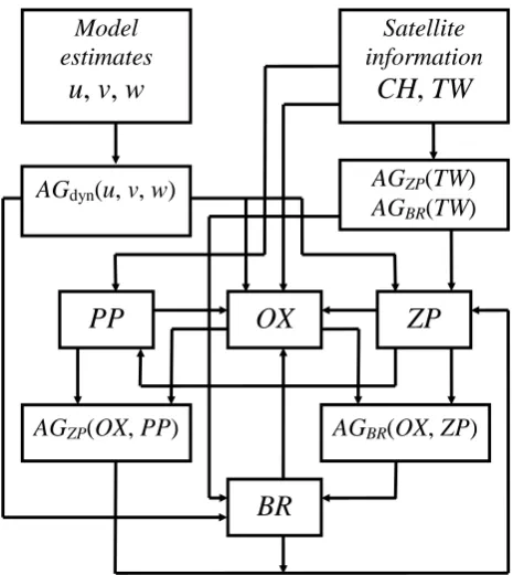
bioresource concentration means all the living objects above the zooplankton in the food chain. The assessments of advection and diffusion obtained from the calcula-tions of current velocity components u, v and w by the hydrodynamic model and also the satellite observations data on sea surface temperature TW and chlorophyll-a concentrchlorophyll-ation СН are used as the external influencesA_i. The scheme of intersys-tem and external influences (conceptual model) of ecosysintersys-tem is represented in Fig. 1.

The ecosystem model contains resource limitation agents (6) of aquatic organ-ism concentration in the food chain AGZP(OX,PP) and AGBR(OX,ZP), concen-tration change monitoring agents of oxygen AGdyn(OX), zooplankton AGdyn(ZP)

and bioresource AGdyn(BR) (the concentrations change due to advection and

BR

PP

ZP

Model

estimates

u

,

v

,

w

Satellite information

CH

,

TW

AGdyn(u, v, w) AGZP(TW)

AGBR(TW)

AGZP(OX, PP) AGBR(OX, ZP)

OX

Fig. 1. Conceptual model of the sea upper layer ecosystem

To construct the system of equations of ecosystem adaptive model,

corres-ponding to conceptual model (Fig. 1), the common АВС-method equations are

used. For the comparison of scenarios to be easier, model variables were

represented in dimensionless form and were reduced to the common interval of variability (0; 10). At the same time, average values of all variables became equal(Ci=5), and specific rates of variable change were taken to be equal to 1(ri =1). The equations of adaptive ecosystem model take on the following form:

)] (

5 [

2PP PP a _/ CH a _/ ZP

dt dPP ZP PP CH PP + − −

= , (11)

− +

+ −

−

= OX OX AG OX a BR a ZP

dt dOX

ZP OX BR

OX/ / dyn( )

[ 5 { 2 ]} /

/ PP a TW

aOX PP + OX TW

− , (12)

dif dif adv adv

dyn(OX) a OX a OX

AG = + , (13)

)]}, ( ) , ( ) ( [ 5 {

2ZP ZP AGdyn ZP a / BR AG OX PP AG TW

dt dZP

ZP ZP

BR

ZP − −

+ −

−

= (14)

dif dif adv adv

dyn(ZP) a ZP a ZP

AG = + , (15)

)], ( );

( min[

arg a / OX t a / PP t

MZP = ZP OX ZP PP

] ) (

exp[ )

( ZP/TW ZP ZP* 2

ZP TW a TW TW

AG = −α − , (17)

)]}, ( ) , ( ) ( [ 5 {

2BR BR AG_dyn BR AG OX ZP AG TW

dt dBR BR BR − − − −

= (18)

dif dif adv adv

dyn(BR) a BR a BR

AG = + , (19)

], 0 ; ; [ ] 0 ; ; [ ) , ( / / / / ZP a ZP a M IF OX a OX a M IF ZP OX AG ZP BR ZP BR BR OX BR OX BR BR BR = + + = = (20) ] ) ( exp[ )

( _{BR/TW BR BR}* 2

BR TW a TW TW

AG = −α − . (21)

In the equations (11) – (21) the agents AG_dyn(OX), AG_dyn(ZP) and

) (

dyn BR

AG consider the changes of oxygen, zooplankton and bioresource

concen-trations, respectively, which takes place in marine environment unit volume due to

advection and diffusion of substances in this volume. AGZP(TW) and

) (TW

AG_BR agents control the degree of the sea upper layer temperature effect on the change of zooplankton and bioresource concentrations, respectively. At the values of TWZP* =TWBR* =26°С the most favorable conditions for the increase of these concentrations are set.

It should be noted that phytoplankton advection and diffusion are indirectly taken into consideration in the equation (11), because the satellite measurement data on СН chlorophyll-a concentration, formed under effect of advection and dif-fusion, had been used as an external influence source in this equation. Through sys-tem of equations of the model this influence is also extended to other model va-riables. However, it is insignificant due to the fact that the influence of previous resource factors decreases with each transition to the new reaction. This is the cause of diffusion and advection inclusion in all other model equations. Current velocities and turbulent exchange coefficients, taken from the calculations by the hydrodynamic model, introduce an additional data on environment dynamics to the ecosystem model because during the calculation of currents the observational data on temperature and salinity fields, shear stress of wind friction and heat flows on the sea surface and also boundary conditions etc. are used. Therefore the manage-ment agents AGdyn(OX) and AGdyn(BR) are the additional sources of influences

on the substance concentration changes in the equations (12), (14) and (18).

1954 – 2007. These data allow us to adopt the following concentration values as estimations of field average values: CPP= 6 g/m

3

and CZP= 0.2 g/m

3

.

a b

Fig. 2. The change of phytoplankton biomass (g/m3) in 1954 – 2005 [8] (a) and biomasses (mg/m3) of edible zooplankton and Noctiluca scintillans in 1953 – 2007 [9] (b) at the BS NWS

The data on bioresource concentration monitoring are quite scattered and be-long, in general, to the Dnieper and the Danube estuarine regions. For an approx-imate estimation of CBR value the results of edible and gelatinous zooplankton biomass monitoring in these regions (given in Fig. 3) are used. Relying on these data and also on the materials of [10], the value CBR = 0.1 g/m

3

was adopted as an estimation of bioresource concentration average value.

Fig. 3. Biomass (mg/m3) of edible and gelatinous zooplankton and Noctiluca scintillans in the Da-nube (a) and Odessa (b) regions during 2003 – 2007 [9]

of the rivers. Therefore the value equivalent to C_OX= 7 ml/l [11, 12] was adopted as an estimation of average annual oxygen concentration.

The obtained approximate estimates of average values of concentrations al-lowed us to calculate the coefficients of intersystem influences in the ecosystem model using the formula (10). The coefficients of CH chlorophyll-а and TW water temperature are selected from considerations of computational stability. Their ab-solute values are represented in the table.

The values of coefficients of intersystem and external influences

aMM/NN PP OX ZP BR CH TW

PP 1 0 0 0 0.8 0

OX 0.5 1 0.3 0.2 0 0.9

ZP 0.27 0.23 1 0.5 0 0.6

BR 0 0.14 0.49 1 0 0.6

To construct the charts of the sea upper layer ecosystem fields in the BS NWS region there were used the scenarios of inter annual variability concentrations of chlorophyll-a, temperature and horizontal velocities of currents, calculated for each node of a square grid (which covered this region) with 5 km step according to the data of satellite observations for 2012 posted on a web-site http://www.myocean.eu/ [13]. Grid domain included 4004 nodes. The calculations of ecosystem fields were performed for 366 calculation time steps (days).

Calculations of ecosystem variables were carried out in two stages. Initially, the model equations (11) – (21) were solved in each nod of the grid domain with no regard for advection and diffusion. As a result, the scenarios of within-year varia-tion of all ecosystem parameters, by which the charts of substance concentravaria-tion spatial distributions for each day were constructed subsequently, had been calcu-lated. These data, alongside with the calculations of horizontal currents, were used to obtain the advection and diffusion assessments in each node of grid domain for each day of experiment. Advection and diffusion were calculated by standard fi-nite-difference formulas.

At the second stage the local adaptation of model variables to the obtained ad-vection and diffusion assessments was performed by means of model (11) – (21). These assessments were included into the management agents (13), (15) and (19), and influence coefficients in management agents AGdyn had the meaning of time

intervals during which the advective and diffusive supplements to the concentra-tions of substances. Thus, the assessments of advection and diffusion have served as additional sources of external influences in the ecosystem model equations.

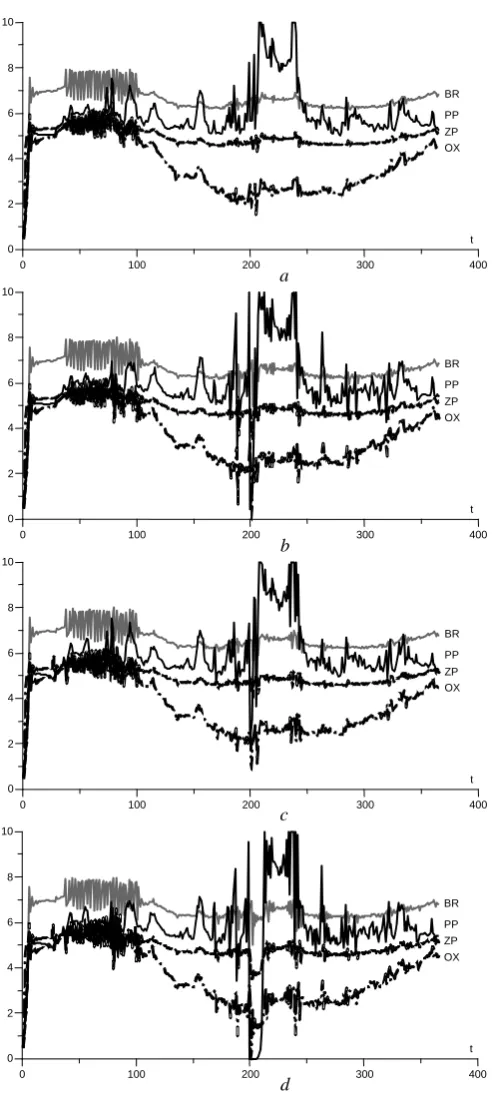
0 2 4 6 8 10

0 100 200 300 400

t BR

OX ZP PP

0 2 4 6 8 10

0 100 200 300 400

t BR

OX ZP PP

0 2 4 6 8 10

0 100 200 300 400

t BR

OX ZP PP

0 2 4 6 8 10

0 100 200 300 400

t BR

OX ZP PP a

b

c

d

From the analysis of the graphs represented in Fig. 4, a it follows that the main contribution to the biochemical process variability was made by the data on chlo-rophyll-a concentration and seasonal sea temperature variation. As expected, the scenario of phytoplankton concentration PP appeared to be the most sensitive one. Summer temperature maximum sufficiently affected the scenario of oxygen con-centration OX. At the same time, this maximum did not affect zooplankton ZP and bioresource BR scenarios due to resource limitations of concentration increase, which were performed by AGZP(OX,PP) and AGBR(OX,ZP) management

agents. The scenarios of ZP and BR concentrations were affected by oxygen con-centration ОХ because of minimum values of oxygen concentration which had been observed in this nod of grid domain almost all year long.

The advection influence on the scenarios excluding the diffusion is represented in Fig. 4, b. This influence appeared to be rather weak. It manifested itself in the increase of phytoplankton and oxygen concentration variability. The diffusion in-fluence excluding the advection (represented in Fig. 4, c) had a bit stronger effect. In both cases the changes have affected phytoplankton and oxygen scenarios.

Scenarios shown in Fig. 4, d demonstrate a joint effect of taking into account advection and diffusion. The feature of these scenarios is a sharp minimum of phy-toplankton concentration occurred on the 210th day of computation. In Fig. 4, a this minimum is absent, and this fact confirms its dependence on the dynamic processes in the sea. Resource limitation agents transformed the minimum of phytoplankton concentration PP into the minima of zooplankton ZP and bioresorce BR concentra-tions.

The analysis of ecosystem variable temporal scenarios confirmed the model sensitivity to the satellite data and information on marine environment dynamics obtained from the calculations performed by hydrodynamical model. The coeffi-cients of influences, applied in computational experiments, were used at the second stage of calculations during the computation of scenarios in all nodes of grid do-main to construct the charts of ecosystem fields.

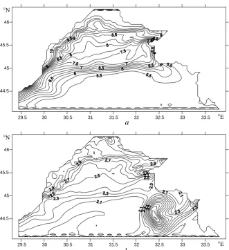
°E

29.5 30 30.5 31 31.5 32 32.5 33 33.5

29.5 30 30.5 31 31.5 32 32.5 33 33.5

°N

44.5 45 45.5 46

44.5 45 45.5 46

а

°N

44.5 45 45.5 46

°E

29.5 30 30.5 31 31.5 32 32.5 33 33.5

b

°N

44.5 45 45.5 46

°E

29.5 30 30.5 31 31.5 32 32.5 33 33.5

c

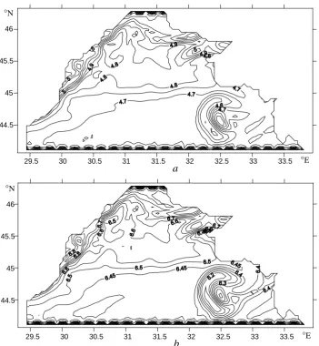
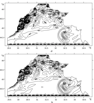
In Fig. 6, a chart of phytoplankton concentration field, constructed without taking into account the marine environment dynamics by the temporal scenarios calculated in the nods of grid domain, is given. The structure of isolines on this chart basically follows the one from Fig. 5, b (the chart of chlorophyll-a concentra-tion fields constructed according to the satellite data).

°N

44.5 45 45.5 46

°E

29.5 30 30.5 31 31.5 32 32.5 33 33.5

a

°E

29.5 30 30.5 31 31.5 32 32.5 33 33.5

b

°N

44.5 45 45.5 46

Fig. 6. Charts of phytoplankton (a) and oxygen (b) concentrations calculated in dimensionless units on the 210th day of computations excluding marine environment dynamics

°N

44.5 45 45.5 46

°E

29.5 30 30.5 31 31.5 32 32.5 33 33.5

a

°N

44.5 45 45.5 46

°E

29.5 30 30.5 31 31.5 32 32.5 33 33.5

b

Fig. 7. Charts of zooplankton (a) and bioresource (b) calculated in dimensionless units on 210th day of computation excluding the marine environment dynamics

Considering the influence of resource limitation agents on scenarios of processes shown in Fig. 4, a it was pointed out that oxygen concentration minima play a key role in formation of scenarios of zooplankton and bioresource concen-trations. Therefore, it should be expected that the oxygen field anomaly will manif-est itself in the fields of zooplankton and bioresource as well. The charts of these fields, represented in Fig. 7, a, b, confirm this statement. The greatest zooplankton and bioresource concentrations are observed in the Danube estuary coastal regions and the lowest concentrations – in the area of oxygen field anomaly near the south-western coast of the Crimea.

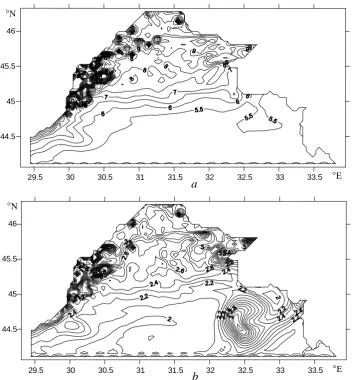
concentrations in Fig. 5, b near the north-western coast of the BS NWS water area, were not visible in the chart of phytoplankton concentration (Fig. 6, a) constructed excluding the water dynamics. Taking into account the dynamics, they explicitly manifested themselves in Fig. 8, a.

°N

44.5 45 45.5 46

°E

29.5 30 30.5 31 31.5 32 32.5 33 33.5

a

°N

44.5 45 45.5 46

°E

29.5 30 30.5 31 31.5 32 32.5 33 33.5

b

Fig. 8. The charts of phytoplankton (a) and oxygen (b) concentrations calculated in dimensionless units on the 210th day of computations taking into account advection and diffusion

°N

44.5 45 45.5 46

°E

29.5 30 30.5 31 31.5 32 32.5 33 33.5

a

°N

44.5 45 45.5 46

°E

29.5 30 30.5 31 31.5 32 32.5 33 33.5

b

Fig. 9. The charts of zooplankton (a) and bioresource (b) concentrations calculated in dimensionless units on the 210th day of computations taking into account advection and diffusion

to the data of satellite observations and assessments of advection and diffusion (calculated according to marine environment numerical modeling data). It is shown that the fact of taking into account the marine environment dynamics and resource limitation agents in the ecosystem adaptive model makes possible the charts of bio-chemical fields to be presented in more details. The proposed method in its further development may provide an alternative to the method of biochemical field calcu-lation using the complex partial differential equations of “reaction – advection – diffusion” type in numerical modeling of marine ecosystem dynamics.

REFERENCES

1. Korotaev, G.K., Oguz, T. & Dorofeyev, V.L. [et al.], 2011, “Development of Black Sea now-casting and forenow-casting system”, Ocean Sci., no. 7, pp. 629-649.

2. Mizyuk, A.I., Knysh, V.V. & Kubryakov, A.I. [et al.], 2010, “Assimilation of the climatic hydrological data in the σ-coordinate model of the Black Sea by the algorithm of adaptive sta-tistics”, J. Phys. Oceanogr., no. 6, pp. 339-357.

3. Korotaev, G.K., Eremeev ,V.N., 2006, “Vvedenie v operativnuyu okeanografiyu Chernogo morya”, Sevastopol, EKOSI-Gidrofizika, 382 p. (in Russian).

4. Timchenko, I.E., Ivashchenko, I.K. & Igumnova, E.M. [et al.], 2014, “Uchet dinamiki i re-sursnykh svoystv morskoy sredy v adaptivnykh modelyakh morskikh ekosistem [Consideration of dynamics and resource properties of marine environment in marine ecosystem adaptive models]”, Morskoy gidrofizicheskiy zhurnal,no. 4, pp. 51-67 (in Russian).

5. Timchenko, I.E., Igumnova, E.M. & Timchenko, I.I. [et al.], 2000, “Sistemnyy menedzhment i AVS-tekhnologii ustoychivogo razvitiya”, Sevastopol, MGI NAN Ukrainy, 225 p. (in Rus-sian).

6. Timchenko, I.E., Igumnova, E.M., 2003, “Modelirovanie protsessov adaptatsii v ekosiste-makh [Modeling of adaptation processes in the ecosystems]”, Morskoy gidrofizicheskiy zhur-nal, no. 1, pp. 46-57 (in Russian).

7. Ivanov, V.A., Igumnova, E.M. & Timchenko, I.E., 2012, “Coastal Zone Resources Manage-ment”, Kyiv, Akademperiodika, 304 p.

8. Nesterova, D., Moncheva, S. & Mikaelyan, A. [et al.], 2008,“The state of phytoplankton”, State of the Enviroment of the Black Sea 2001– 2006/7, Chief ed. T. Oquz., Commission on the Protection of the Black Sea Against Pollution. Report, Turkey, Istanbul, ch. 5, pp. 173-200.

9. Shiganova, T., Musaeva, E. & Arashkevich, E. [et al.], 2008, “The state of zooplankton”, State of the Enviroment of the Black Sea 2001– 2006/7, Chief ed. T. Oquz., Commission on the Protection of the Black Sea Against Pollution. Report, Turkey, Istanbul, ch. 6, pp. 201-246.

10. Latun, V.S., 2012, “Vliyanie rybnogo promysla na ustoychivost' ekosistemy Chernogo morya

[The impact of fisheries on the Black Sea ecosystem stability]”, Ustoychivost' i evolyutsiya okeanologicheskikh kharakteristik ekosistemy Chernogo morey, pp. 331-353 (in Russian). 11. Emelyanov, V.A., Mitropol'skiy, A.Yu. & Nasedkin, E.I. [et al.], 2004, “Geoekologiya

cher-nomorskogo shel'fa Ukrainy”, Kiev, Akademperiodika, 296 p. (in Russian).

12. Orlova, I.G., Pavlenko, M.Yu. & Ukraїns'kiy, V.V., 2008, “Gidrologichni ta gidrokhimichni pokazniki stanu pivnichno-zakhidnogo shel'fu Chornogo morya: dovidkoviy posibnik”, Kiiv, KNT, 616 p. (in Ukranian).