* Corresponding author. Tel.: +091-033-2414-6153
E-mail: [email protected] (S. Chakraborty) © 2013 Growing Science Ltd. All rights reserved.
doi: 10.5267/j.ijiec.2013.03.007
Contents lists available at GrowingScience
International Journal of Industrial Engineering Computations
homepage: www.GrowingScience.com/ijiec
A solution to robot selection problems using data envelopment analysis
Suprakash Mondala and Shankar Chakrabortyb*
a Department of Production Engineering, Mallabhum Institute of Technology, Bishnupur, Bankura – 722 122, West Bengal, India bDepartment of Production Engineering, Jadavpur University, Kolkata – 700 032, West Bengal, India
C H R O N I C L E A B S T R A C T
Article history: Received January 8 2013 Received in revised format March 15 2013
Accepted March 18 2013 Available online March 23 2013
Selection of industrial robots for the present day’s manufacturing organizations is one of the most difficult assignments due to the presence of a wide range of feasible alternatives. Robot manufacturers are providing advanced features in their products to sustain in the globally competitive environment. For this reason, selection the most suitable robot for a given industrial application now becomes a more complicated task. In this paper, four models of data envelopment analysis (DEA), i.e. Charnes, Cooper and Rhodes (CCR), Banker, Charnes and Cooper (BCC), additive, and cone-ratio models are applied to identify the feasible robots having the optimal performance measures, simultaneously satisfying the organizational objectives with respect to cost and process optimization. Furthermore, the weighted overall efficiency ranking method of multi-attribute decision-making theory is also employed for arriving at the best robot selection decision from the short-listed competent alternatives. In order to demonstrate the relevancy and distinctiveness of the adopted DEA-based approach, two real time industrial robot selection problems are solved.
© 2013 Growing Science Ltd. All rights reserved Keywords:
Robot selection
Data envelopment analysis CCR model
BCC model Additive model Cone ratio model
1. Introduction
come back to a programmed location; load capacity indicates the weight (load) a robot can pick up; speed is defined as how quickly a robot can position its arm/actuator and accuracy is understood as how closely a robot can attain a commended point. Among these criteria, some are advantageous in nature (beneficial) and some are non-advantageous (non-beneficial). For beneficial criteria, like load capacity and program flexibility, higher values are always desirable, whereas, for non-beneficial criteria, like cost and repeatability, lower values are preferable. Due to availability of a wide range of robots in the market, selection of the most suitable robot for a specific application becomes a challenging task. Improper selection of robot may not only adversely affect productivity and quality of products but also the reputation of the manufacturing organizations is negatively affected. However, executing the application of a robot is a capital-intensive job. Therefore, prior to its implementation, a vigilant examination regarding its practicability and performance is required, in which the impact of various selection criteria should be assessed. While selecting the most suitable robot for a given application, the decision maker requires to consider different robot selection attributes, which often involve swapping between a varieties of robot performance measures. Numerous approaches, including multi-criteria decision-making (MCDM) methods and optimization techniques have already been proposed by the past researchers for robot selection. Decision analysis is primarily concerned with those circumstances where a decision maker has to opt for the best alternative amongst several competent alternatives at the same time considering a set of conflicting criteria. In order to weigh up the overall effectiveness of the candidate alternatives and select the most suitable robot, the primary objective of an MCDM approach is thus to identify the significant robot selection criteria for a given application, assess the information relating to those criteria and develop methodologies for evaluation to meet the decision maker’s requirements.
2. Review of literature
Liang and Wang (1993) combined fuzzy set theory and hierarchical structure analysis for solving robot selection problems. Khouja and Booth (1995) proposed a decision model for robot selection using fuzzy cluster analysis. Khouja (1995) applied a two-phase model for solving robot selection problems. In the first phase, data envelopment analysis (DEA) was used to identify the feasible robot alternatives based on satisfaction of some predefined performance measures and in the second phase, an MCDM model was employed to select the best robot from those identified in the first phase. Goh et al. (1996) presented a revised weighted sum model incorporating the values assigned by a group of experts on different factors for selecting industrial robots.
Karsak (1998) proposed a two-phase methodology for robot selection. In the first phase, DEA was used to determine the technically efficient robot alternatives, considering cost and technical performance parameters. In the second phase, a fuzzy robot selection algorithm was applied to rank the technically efficient robots based on both predetermined objective criteria and additional vendor-related subjective criteria. Goh (1997) applied analytic hierarchy process (AHP) for solving robot selection problems having both subjective and objective data for alternative robot evaluation. Parkan and Wu (1999) compared the performance of OCRA (Operational Competitiveness RAting) and TOPSIS (Technique for Order Preference by Similarity to Ideal Solution) methods through a robot selection problem. It was proposed to make the final selection on the basis of rankings obtained by averaging the results of OCRA, TOPSIS and a utility model.
of dimensional analysis (DA) for robot selection. The proposed DA approach would provide an easy, efficient and robust decision support system overcoming all attribute dimension problems. Chu and Lin (2003) applied a fuzzy TOPSIS method for robot selection, where the ratings of various alternatives with respect to different subjective criteria and weights of all criteria were assessed in linguistic terms using fuzzy numbers.
Bhangale et al. (2004) developed a reliable and exhaustive database of robot manipulators to standardize the robot selection procedure, and help the robot user for selecting the most appropriate robot system to meet the operational requirements. Bhattacharya et al. (2005) integrated AHP and quality function deployment (QFD) model to justify the implementation of a robotic system in a manufacturing organization. Karsak and Ahiska (2005) solved the robot selection problems using the cross-efficiency analysis of DEA method. The proposed methodology would enable evaluation of the relative efficiency of decision-making units with respect to multiple outputs and a single exact input. Rao and Padmanabhan (2006) proposed a digraph and matrix-based approach for evaluation of alternative industrial robots. A robot selection index was suggested to evaluate and rank the robots for a given industrial application.
Kahraman et al. (2007) used a fuzzy hierarchical TOPSIS model for multi-criteria evaluation of the industrial robotic systems. Karsak (2008) introduced a decision model for robot selection based on QFD and fuzzy linear regression. Shih (2008) evaluated the performance of alternative robots based on an incremental benefit-cost ratio model and then ranked the robots using group TOPSIS method. Kumar and Garg (2010) developed a distance-based approach for evaluation, selection and ranking of robots. Chatterjee et al. (2010) solved two real time robot selection problems using VIKOR (VIsekriterijumsko KOmpromisno Rangiranje) and ELECTRE (ELimination and Et Choice Translating REality) methods, and also compared their relative performance.
Rao et al. (2011) applied a subjective and objective-integrated MCDM method for the purpose of robot selection. Alinezhad et al. (2011) integrated MCDM and DEA methods in order to evaluate the relative efficiency of alternative robots with respect to multiple outputs and a single input. Athawale & Chakraborty (2011) compared the ranking performance of ten most popular MCDM methods while solving an industrial robot selection problem. It was concluded that for a given robot selection problem, more attention should be given on proper selection of criteria and alternatives, not on choosing the most appropriate MCDM method to be employed. Koulouriotis and Ketipi (2011) developed a digraph model for evaluation of the alternative robots and selection of the most appropriate one from the feasible alternatives. Devi (2011) extended VIKOR method in intuitionistic fuzzy environment for solving MCDM problems in the area of robot selection. Athawale et al. (2012) applied VIKOR method for evaluating and ranking of industrial robots. Karsak et al. (2012) presented a decision model based on fuzzy linear regression for industrial robot selection.
It is observed that the past researchers have adopted different variants of DEA method to solve the robot selection problems. No attempt has yet been made to compare the ranking performance and solution accuracy of various DEA models. This paper evaluates the performance of four commonly employed DEA models while solving two real time robot selection problems.
3. Data envelopment analysis
efficiency of a DMU, most of the DEA models assign the score of 1 to the efficient DMUs with respect to other inefficient DMUs. Generally, a DMU is held responsible for converting inputs into outputs for evaluating its performance scores (Cooper et al., 2011; Roghanian & Foroughi, 2010). The main advantage of DEA lies in its ability to deal with multiple inputs and outputs having different units. It also does not require any particular functional form related to inputs and outputs. In spite of having these advantages, DEA models have some limitations too. Being a non-parametric mathematical technique, statistical hypothesis tests are difficult to perform and the LP formulations associated with DEA models may be sometimes computationally intensive. Although there are several DEA models, this paper mainly focuses on the application of four most potential models, i.e. Charnes, Cooper and Rhodes (CCR), Banker, Charnes and Cooper (BCC), additive, and cone-ratio models.
3.1 CCR model
The CCR model is the most basic and widely applied model of DEA. This model was first introduced by Charnes, Cooper and Rhodes in 1978, from the earlier work of Farell on a basic theory of productivity measurement using single output and single input ratio concept (Cooper et al., 2011). Basically, the CCR model is the extension of Farell’s model to measure organizational efficiency by using multiple outputs/multiple inputs ratio concept with no priori information about the relative importance on inputs and outputs. The main objective of CCR model is to identify the corresponding efficient DMUs against each inefficient DMU (Kuah et al., 2010). A DMU is more efficient if it can create a larger number of outputs with the same quantity of inputs (output-oriented approach) or vice versa (input-oriented approach).
Let, there are n number of alternatives (DMU) to be evaluated on the basis of some conflicting input criteria (non-beneficial) and output criteria (beneficial). There are m number of input criteria for each alternative denoted by xik (for i = 1,…,m) and s is the number of output criteria for each alternative
denoted by yrk (for r = 1,…,s). xik and yrk denote the values of ith input criterion and rth output criterion
for kth alternative. The basic fractional non-convex programming mode of CCR model can be expressed
by the following equations (Cooper et al., 2011).
m i ik i s r rk r i r k x v y u v u H 1 1 max subject to∑∑
∑∑
1 1 1 1 1 ≤ ) ( ) ( m i n j ij i s r n j rjry vx
u
(1)
ur> 0, r = 1,…,s
vi > 0, i = 1,…,m
(2)
where yrjis the value of jth alternative on rth output criterion and xij is the value of ith input for jth
alternative. ur and vi are the non-negative variable weights to be determined by the solution of the
above maximization problem. The above fractional non-convex programming model is computationally much difficult to solve for the decision maker. To overcome the computational difficulties of Eq. (1) and Eq. (2), Charnes et al. (1978) developed a LP model of CCR approach. This LP model can be articulated either by maximizing output criteria or minimizing input criteria values. In this paper, the input minimization formulation of CCR model is adopted as given below.
m i ik ik vx
g
1
) min(
s
r
m
i ik i rk
ry vx
u
1 1
0 for j = 1,…,n (3)
s
r rk ry u
1
1 (4)
ur≥ 0, r =1,…,s
vi≥ 0, i = 1,…,m
(5)
Charnes et al. (1978) also adopted the following expression to compute the efficiency measures.
Hk = 1/gk, (6)
where Hk is the efficiency measure of kth DMU. In CCR model, a DMU is considered efficient if it
achieves a score of 1, otherwise, it is treated as inefficient. The identified efficient DMUs act as a benchmarking standard for future improvements. Although the CCR model is the simplest DEA model, but its major disadvantage lies in the fact that an inefficient DMU and its benchmarking DMU may not be same in their operations (Kuah et al., 2010).
3.2 BCC model
The BCC model of DEA was first initiated by Banker in 1984 (Banker et al., 1984). In BCC model, if all the inputs are changed by equal proportion, there will be a huge change in the outputs crossing the proportional limit by a great extent. This property of BCC model is known as variable return to scale (VRS). The basic difference between BCC and CCR models lies in the fact that CCR model works on the concept of constant return to scale (CRS) which can be defined as scaling the inputs and outputs linearly without increasing or decreasing efficiency (Ramanathan, 2003). Additional convexity constraint (∑λj = 1) is also added in this model. The BCC model scores higher efficiency as compared
to CCR model. Generally, a DMU is BCC efficient if it is CCR efficient, but it is not required that a BCC efficient DMU is CCR efficient (Cook & Seiford, 2009). The input-oriented minimization formulation of BCC model is shown as below (Banker et al., 1984):
min G0
subject to
j
i ij
jx G0x0 0
(7)
j
r rj
jy y0 0
(8)
1
j j
(9)
λj≥ 0,
where yrj is the amount of rth output for jth DMU and xijis the amount of input for the same DMU. λ is
the non-negative vector. The BCC model evaluates the efficiency of Oth DMU (O = 1,...,n) by solving
the above LP problem. A DMU is BCC efficient if it has a relative efficiency score of 1, and a relative efficiency score less than 1 shows the inefficiency of the DMU.
3.3 Additive model
simultaneously (Sun & Gui, 2011). The basic models of DEA, like CCR and BCC belong to radial category, whereas, additive model belongs to non-redial category. The additive model of DEA was first introduced and advocated by Charnes et al. (Charnes et al., 1985). The additive model is also known as welfare efficiency model or Pareto-Koopmans efficiency model as it is not possible to improve any input or output without worsening some other inputs or outputs. The unique characteristic of additive model is that it can shift an inefficient DMU to the efficient boundary. As the additive model combines both input-oriented and output-oriented approaches, it considers slacks (input excesses and output shortfalls) directly in the objective function. A DMU is said to be additive efficient if its all slacks become zero at its optimal solution (Cook & Seiford, 2009). There are several forms of additive model in DEA literature and the most basic form of the additive model is shown in Eqn. (10) in LP format. Consider there are n DMUs, i.e. DMU1, DMU2,…,DMUn. Each DMUj (j = 1,…,n) uses m inputs xij (i =
1,…,m) and generates s outputs yrj (r = 1,…,s).
i r
r
i S
S
P0 Max
subject to
,
0
i i j
ij
jx S x
i = 1,…,m (10),
0
r r j
rj
jy S y
r = 1,…,s (11)1
j j
(12)
λj, Si-, Sr+ ≥ 0, i,j,r
where Si- and Sr+ are the slacks, Si- is the input excess and Sr+ is the output shortfall. The DMUj to be
evaluated on any trial is designated as DMUo (o = 1,…,n) and λ is the non-negative vector. The
efficiency of each DMUo and the value of Po are thus found by solving the LP models.
3.4 Cone-ratio model
The fundamental concept of cone-ratio DEA (CRDEA) is based on the principle of assurance region (AR) (Charnes et al., 1990). Similar to AR philosophy, CRDEA approach allows for weight restrictions which ultimately improve the discriminating power of DEA. These weight restrictions are specified by linear inequalities defining bounds on weights which reflect the importance of inputs and outputs, and ultimately lead to the development to CRDEA model with input and output cones specified by their respective weight restrictions. There are several forms and extensions of DEA, but the cone-ratio approach makes it possible to enhance both the power and flexibility of DEA by recourse to supplementary information to effect data adjustments which can be brought to allow in carrying out evaluations from the acceptable solutions (Brockett et al., 1997). In CRDEA model, the number of cones depends on the number of beneficial attributes. If s is the number of beneficial attributes considered, then the number of cones will be factorial s. Here, the output maximization formulation of CRDEA model is shown as below.
m
j jq j s
k kq k
x u
y v
1 1
Max
(13)
where qth DMU is being evaluated. Here, s, m and n represent the output, input and number of DMUs respectively, yki and xji are the amount of kth output and jth input respectively for ith DMU, vk and uj are
the variable weights, and γ, δ, c and d are the non-negative scalars. The above fractional program can be transformed into LP problem to solve it easily.
s k kq ky v 1 Max (18) subject to
m j jq jx u 1 1 (19)
s k m j ji j kiky u x
v
1 1
0 i (20)
γju1 - uj≤ 0, j = 2,…,m δju1 - uj≥ 0, j = 2,…,m
ckv1 - vk≤ 0, k = 2,…,s
dkv1 - vk≥ 0, k = 2,…,s
uj, vk≥ 0 k,j
To determine the relative efficiencies of DMUs, the above LP problem is required to be solved n
number of times. The efficiency values of DMUs come from the efficiency scores of the individual DMUs. A relative efficiency score of 1 signifies that the DMU is efficient, however, a relative efficiency score less than 1 signifies that the DMU is inefficient. Although the CRDEA model can effectively integrate the decision maker’s preferences, but it is unable to solve the problems with multiple optimal solutions (Talluri & Yoon, 2000).
3.5 Weighted overall efficiency ranking method
Let α designate a unit and Β denote the set of all the performance units. With each unit α in B associate
k attributes (variables or performance measures) X1,…, Xkwhose values are denoted by x1,…, xk. The
problem is to choose α in B so that the decision maker is the happiest with the payoff x1,…, xk. Thus, an
index that combines X1,…, Xkinto a scalar quantity, u of preferability or value is needed. To solve the
above problem, a scalar-valued function, u(X1,…,Xk) that models the decision maker’s preference for
the attributes is estimated. The function, u is also referred to as a utility function, a worth function or a preference function. When the attributes are mutually preferentially independent, the function
u(X1,…,Xk) is additive. Preferential independence can be illustrated as follows: suppose, while making
decision for robot selection, the decision maker is concentrated with only two criteria of the robot, e.g. repeatability and cost. If the decision maker’s preference for repeatability is independent of cost and when this independence relation holds for both the attributes, they are mutually preferentially independent. Thus, the additive utility function, when the attributes are mutually preferentially independent, can be given as below:
k i i ik u X
X X u
1
1,..., ) ( )
( , (21)
1 Max 1 1
m j ji j s k ki k x u y v, i
(14)
γju1≤uj≤δju1, j = 2,…,m (15)
ckv1≤vk≤dkv1, k = 2,…,s (16)
where ui(Xi) is the single-attribute utility function for ith performance measure. For non-beneficial
attributes, the single-attribute utility function can be defined as follows: )
/( ) (
)
( max max min
i i
i i
i
i X X X X X
u , (22)
where max
i
X and min
i
X are the highest and lowest values of ith attribute respectively.
On the other hand, for beneficial attributes, the single-attribute utility function can be expressed as:
5 . 0 min max
min)/( )]
[( )
( i i i i i
i X X X X X
u . (23)
With an additive value function, the utility value that the decision maker obtains from a unit with performance measure, x1,…, xkis equal to the sum of the utility which is obtained from each measure
for that unit. Thus, the decision maker’s preference for the performance measures can be evaluated individually which simplifies their assessment. Furthermore, as the single-attribute utility function,
ui(Xi) is usually non-linear, thus it better captures the preference of the decision maker. The additive
utility function, u(X1,…,Xk) and the single-attribute utility function, ui(Xi) are usually scaled from 0 to 1
for convenience, i.e.
0 ≤u(X1,…,Xk) ≤ 1 and 0 ≤ui(xi) ≤ 1
It results in the additive utility function of the following form:
k i i i ik wu X
X X u
1
1,..., ) ( )
( (24)
where 1
1
k i iw and wi > 0for all i.
Here wi is the scaling constant and can be thought of as the weight associated with ith attribute. Thus,
the unit selection problem using the MCDM theory is to find the unit α in B that maximizes the additive utility function as expressed below:
k i i i ik Max wu X
X X u Max
1
1,..., ) ( )
( , (25)
where Xiis a variable denoting the value of ith performance measure (attribute) associated with the units
and u(X1,…,Xk) is the overall utility function evaluated at (X1,…,Xk). The value of the scaling constant
can be obtained by asking the decision maker to rate the important of each attribute relative to the most important attribute which receives a weight of 100 (Khouja, 1995).
4. Illustrative examples
In order to demonstrate the applicability and solution accuracy of the four considered DEA methods, the following two robot selection problems are cited.
4.1 Example 1
only non-beneficial attribute. In this example, repeatability is considered as input and others are considered as output variables. The decision matrix with seven robot alternatives and five selection criteria is shown in Table 1. Here, four popular DEA models are first applied to identify the efficient robots and then a weighted overall efficiency-based method is employed to determine the final ranking of the efficient robots.
Table 1
Robot selection decision matrix for example 1(Bhangale et al., 2004)
Robot LC (in kg) (in mm) RE (in mm/sec) MTS MC (in points or steps) MR (in mm)
ASEA-IRB 60/2 60 0.4 2540 500 990
Cincinnati Milacrone T3-726 6.35 0.15 1016 3000 1041
Cybotech V15 Electric Robot 6.8 0.1 1727.2 1500 1676
Hitachi America Process Robot 10 0.2 1000 2000 965
Unimation PUMA 500/600 2.5 0.1 560 500 915
United States Robots Maker 110 4.5 0.08 1016 350 508
Yaskawa Electric Motoman L3C 3 0.1 1778 1000 920
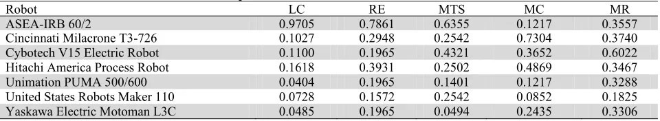
Table 2
Normalized decision matrix for example 1
Robot LC RE MTS MC MR
ASEA-IRB 60/2 0.9705 0.7861 0.6355 0.1217 0.3557
Cincinnati Milacrone T3-726 0.1027 0.2948 0.2542 0.7304 0.3740
Cybotech V15 Electric Robot 0.1100 0.1965 0.4321 0.3652 0.6022
Hitachi America Process Robot 0.1618 0.3931 0.2502 0.4869 0.3467
Unimation PUMA 500/600 0.0404 0.1965 0.1401 0.1217 0.3288
United States Robots Maker 110 0.0728 0.1572 0.2542 0.0852 0.1825
Yaskawa Electric Motoman L3C 0.0485 0.1965 0.0494 0.2435 0.3306
The decision matrix, as shown in Table 1, is first normalized to transform all the criteria values into dimensionless and comparable units, ranging from 0 to 1. The normalized decision matrix is exhibited in Table 2. The main objective of DEA-CCR model is to identify the most feasible alternatives by maximizing the output criteria or by minimizing the input criteria. Eqns. (1) and (2) show the basic non-convex programming models for DEA-CCR approach which can be restructured as LP models using Eqns. (3)-(5). Now, to obtain the efficiency score for each robot alternative, Eqns. (3)-(5) are solved for seven robot alternatives using the data of the normalized decision matrix of Table 2. A model mathematical formulation for robot alternative 1 (ASEA-IRB 60/2) is shown in Table 3.
Table 3
Mathematical modeling of CCR model for ASEA-IRB 60/2 robot min g = 0.7861v1
subject to
-0.9705u1 - 0.6355u2 - 0.121u3 - 0.3557u4 + 0.7861v1 ≥ 0, -0.1027u1 - 0.2542u2 - 0.7304u3 - 0.3740u4 + 0.2948v1 ≥ 0
-0.1100u1 - 0.4321u2 - 0.3652u3 - 0.6022u4 + 0.1965v1 ≥ 0, -0.1618u1 - 0.2502u2 - 0.4869u3 - 0.3467u4 + 0.3931v1 ≥ 0
-0.0404u1 - 0.1401u2 - 0.1217u3 - 0.3288u4 + 0.1965v1 ≥ 0, -0.0728u1 - 0.2542u2 - 0.0852u3 - 0.1825u4 + 0.1572v1 ≥ 0
-0.0485u1 - 0.0494u2 - 0.2435u3 - 0.3306u4 + 0.1965v1 ≥ 0, 0.9705u1 + 0.6355u2 + 0.1217u3 + 0.3557u4 = 1
Objective function value (g) is 1.0000.
The developed LP problem is solved using LINDO software (version 6.1) and the derived efficiency score of ASEA-IRB 60/2 robot is shown in Table 4. Similarly, the mathematical formulations of all the remaining robot alternatives are solved and their efficiency scores are also enlisted in Table 4.
Table 4
CCR efficiency scores for robot alternatives
Robot Robot 1 Robot 2 Robot 3 Robot 4 Robot 5 Robot 6 Robot 7
From Table 4, it is observed that robot 1 (ASEA-IRB 60/2), robot 2 (Cincinnati Milacrone T3-726) and robot 3 (Cybotech V15 Electric Robot) are the efficient choices among the seven considered alternatives. Now, this robot selection problem is solved using BCC model of DEA. While applying BCC model, the mathematical formulation for each robot alternative is developed using Eqns. (7)-(9). The LP model for the first robot is shown in Table 5. It is also solved using LINDO software and the efficiency scores are given in Table 6. This table shows that robot 1 (ASEA-IRB 60/2), robot 2 (Cincinnati Milacrone T3-726), robot 3 (Cybotech V15 Electric Robot) and robot 6 (United States Robots Maker 110) are the efficient choices.
Table 5
Mathematical modeling of BCC model for ASEA-IRB 60/2 robot Min G
subject to
0.7861G - 0.7861λ1 - 0.2948λ2 - 0.1965λ3 - 0.3931λ4 - 0.1965λ5 - 0.1572λ6 - 0.1965λ 7 ≥ 0
0.9705λ1 + 0.1027λ2 + 0.1100λ3 + 0.1618λ4 + 0.0404λ5 + 0.0728λ6 + 0.0485λ7 ≥ 0.9705
0.6355λ1 + 0.2542λ2 + 0.4321λ3 + 0.2502λ4 + 0.1401λ5 + 0.2542λ6 + 0.0494λ7 ≥ 0.6355
0.1217λ1 + 0.7304λ2 + 0.3652λ3 + 0.4869λ4 + 0.1217λ5 + 0.0852λ6 + 0.2435λ7 ≥ 0.1217
0.3557λ1 + 0.3740λ2 + 0.6022λ3 + 0.3467λ4 + 0.3288λ5 + 0.1825λ6 + 0.3306λ7 ≥ 0.3557 λ1 + λ2 + λ3 + λ4 + λ5 + λ6 + λ7 = 1
Objective function value (G) is 1.0000.
Table 6
BCC efficiency scores for robot alternatives
Robot Robot 1 Robot 2 Robot 3 Robot 4 Robot 5 Robot 6 Robot 7
Efficiency score 1.0000 1.0000 1.0000 0.6888 0.8697 1.0000 0.9131
Further, this robot selection problem is again solved using a non-radial approach of additive model of DEA. The corresponding mathematical models for the seven robot alternatives are developed using Eqns. (10)-(12) and solved using LINDO software. The detailed mathematical formulation for ASEA-IRB 60/2 robot is shown in Table 7.
Table 7
Mathematical modeling of additive model for ASEA-IRB 60/2 robot Max Po = S1- + S1+ + S2++ S3++ S4+
subject to
0.7861λ1 + 0.2948λ2 + 0.1965λ3 + 0.3931λ4 + 0.1965λ5 + 0.1572λ6 + 0.1965λ7 + S1- = 0.7861
0.9705λ1 + 0.1027λ2 + 0.1100λ3 + 0.1618λ4 + 0.0404λ5 + 0.0728λ6 + 0.0485λ7 - S1+= 0.9705
0.6355λ1 + 0.2542λ2 + 0.4321λ3 + 0.2502λ4 + 0.1401λ5 + 0.2542λ6 + 0.0494λ7 - S2+ = 0.6355
0.1217λ1 + 0.7304λ2 + 0.3652λ3 + 0.4869λ4 + 0.1217λ5 + 0.0852λ6 + 0.2435λ7 - S3+= 0.1217
0.3557λ1 + 0.3740λ2 + 0.6022λ3 + 0.3467λ4 + 0.3288λ5 + 0.1825λ6 + 0.3306λ7 - S4+= 0.3557
λ1 + λ2 + λ3 + λ4 + λ5 + λ6 + λ7 = 1
Objective function value (Po) is 0.
As mentioned earlier, a robot alternative is said to be additive efficient if all its slacks become 0 at its optimal solution. The additive efficiency scores of seven robot alternatives are given in Table 8. From this Table 8, it is clearly observed that robot 1 (ASEA-IRB 60/2), robot 2 (Cincinnati Milacrone T3-726), robot 3 (Cybotech V15 Electric Robot) and robot 6 (United States Robots Maker 110) are the additive efficient choices.
Table 8
Additive efficiency scores for robot alternatives
Robot Robot 1 Robot 2 Robot 3 Robot 4 Robot 5 Robot 6 Robot 7
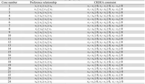
Lastly, this robot selection problem is solved using DEA cone-ratio (CRDEA) model. The previous three DEA-based models do not include the decision maker’s preferences in terms of criteria weights or preference preorder of the criteria. Here, v1, v2, v3 and v4 indicate the relative preferences of LC, MTS,
MC and MR (all beneficial criteria) respectively. There are 24 preference relationships or cones for the four considered beneficial criteria which are given in Table 9. Each cone is used as a set of linear inequality constraints in CRDEA model. In this robot selection problem, among 24 cones, the first cone is developed using the preference order of the beneficial criteria as v1 ≥v2 ≥v3 ≥v4, which indicates that
LC (v1) is preferred to MTS (v2), MTS (v2) is preferred to MC (v3) and MC (v3) is preferred to MR (v4).
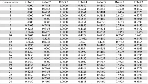
These 24 sets of linear preference relationships are incorporated into CRDEA model. For demonstration purpose, the mathematical model for the first cone of ASEA-IRB 60/2 robot is shown in Table 10. The above-developed mathematical model is solved using LINDO software and the efficiency scores of ASEA-IRB 60/2 robot for 24 cones are given in Table 11. Similarly, the efficiency scores of the remaining alternative robots are calculated, as shown in Table 11. This table identifies Cybotech V15 Electric Robot as the best choice for all the cones.
Table 9
Cones utilized for example 1 (Four variables: v1, v2, v3, v4)
Cone number Preference relationship CRDEA constraint
1 v1 ≥v2 ≥v3 ≥v4 v1 - v2 ≥ 0, v2 - v3 ≥ 0, v3 - v4 ≥ 0
2 v1 ≥v2 ≥v4 ≥v3 v1 - v2 ≥ 0, v2 - v4 ≥ 0, v4 - v3 ≥ 0
3 v1 ≥v4 ≥v2 ≥v3 v1 - v4 ≥ 0, v4 - v2 ≥ 0, v2 - v3 ≥ 0
4 v1 ≥v4 ≥v3 ≥v2 v1 - v4 ≥ 0, v4 - v3 ≥ 0, v3 - v2 ≥ 0
5 v1 ≥v3 ≥v2 ≥v4 v1 - v3 ≥ 0, v3 - v2 ≥ 0, v2 - v4 ≥ 0
6 v1 ≥v3 ≥v4 ≥v2 v1 - v3 ≥ 0, v3 - v4 ≥ 0, v4 - v2 ≥ 0
7 v2 ≥v1 ≥v3 ≥v4 v2 - v1 ≥ 0, v1 - v3 ≥ 0, v3 - v4 ≥ 0
8 v2 ≥v4≥v1≥v3 v2 - v4 ≥ 0, v4 - v1 ≥ 0, v1 - v3 ≥ 0
9 v2 ≥v4 ≥v3 ≥v1 v2 - v4 ≥ 0, v4 - v3 ≥ 0, v3 - v1 ≥ 0
10 v2 ≥v1 ≥v4 ≥v3 v2 - v1 ≥ 0, v1 - v4 ≥ 0, v4 - v3 ≥ 0
11 v2 ≥v3 ≥v1 ≥v4 v2 - v3 ≥ 0, v3 - v1 ≥ 0, v1 - v4 ≥ 0
12 v2 ≥v3 ≥v4 ≥v1 v2 - v3 ≥ 0, v3 - v4 ≥ 0, v4 - v1 ≥ 0
13 v3 ≥v1 ≥v2 ≥v4 v3 - v1 ≥ 0, v1 - v2 ≥ 0, v2 - v4 ≥ 0
14 v3 ≥v1 ≥v4 ≥v2 v3 - v1 ≥ 0, v1 - v4 ≥ 0, v4 - v2 ≥ 0
15 v3 ≥v2 ≥v1 ≥v4 v3 - v2 ≥ 0, v2 - v1 ≥ 0, v1 - v4 ≥ 0
16 v3 ≥v2 ≥v4 ≥v1 v3 - v2 ≥ 0, v2 - v4 ≥ 0, v4 - v1 ≥ 0
17 v3 ≥v4 ≥v2 ≥v1 v3 - v4 ≥ 0, v4 - v2 ≥ 0, v2 - v1 ≥ 0
18 v3 ≥v4 ≥v1 ≥v2 v3 - v4 ≥ 0, v4 - v1 ≥ 0, v1 - v2 ≥ 0
19 v4 ≥v1 ≥v2 ≥v3 v4 - v1 ≥ 0, v1 - v2 ≥ 0, v2 - v3 ≥ 0
20 v4 ≥v1 ≥v3 ≥v2 v4 - v1 ≥ 0, v1 - v3 ≥ 0, v3 - v2 ≥ 0
21 v4 ≥v2 ≥v1 ≥v3 v4 - v2 ≥ 0, v2 - v1 ≥ 0, v1 - v3 ≥ 0
22 v4 ≥v2 ≥v3 ≥v1 v4 - v2 ≥ 0, v2 - v3 ≥ 0, v3 - v1 ≥ 0
23 v4 ≥v3 ≥v2 ≥v1 v4 - v3 ≥ 0, v3 - v2 ≥ 0, v2 - v1 ≥ 0
24 v4 ≥v3 ≥v1 ≥v2 v4 - v3 ≥ 0, v3 - v1 ≥ 0, v1 - v2 ≥ 0
Based on the results derived by the four adopted DEA models, it is clear that CRDEA identifies robot 3 (Cybotech V15 Electric Robot) as a unique choice. On the other hand, CCR, BCC and additive models of DEA short-list some of the robots as efficient ones. To overcome this problem and find out the most suitable robot alternative among the short-listed ones, the weighted overall efficiency ranking method is now employed to rank the efficient robots.
Table 12 exhibits the criteria-wise utility values for three efficient alternative robots. Rao (2007) determined the weights (importance) of the considered robot selection criteria using AHP method, as given in Table 13. Now based on the criteria-wise utility functions of ASEA-IRB 60/2 robot and using Eqs. (24), the overall utility value of that robot is formulated as follows:
Overall utility = w1(LC)xu1(LC) + w2(RE)xu2(RE) + w3(MTS)xu3(MTS) + w4(MC)xu4(MC) +
Table 10
Mathematical modeling of CRDEA model for ASEA-IRB 60/2 (for cone 1) Max 0.9705v1 + 0.6355v2 + 0.1217v3 + 0.3557v4
subject to
0.9705v1 + 0.6355v2 + 0.1217v3 + 0.3557v4 - 0.7861u1 ≤ 0 0.1027v1 + 0.2542v2 + 0.7304v3 + 0.3740v4 - 0.2948u1 ≤ 0
0.1100v1 + 0.4321v2 + 0.3652v3 + 0.6022v4 - 0.1965u1 ≤ 0 0.1618v1 + 0.2502v2 + 0.4869v3 + 0.3467v4 - 0.3931u1 ≤ 0
0.0404v1 + 0.1401v2 + 0.1217v3 + 0.3288v4 - 0.1965u1 ≤ 0 0.0728v1 + 0.2542v2 + 0.0852v3 + 0.1825v4 - 0.1572u1 ≤ 0
0.0485v1 + 0.0494v2 + 0.2435v3 + 0.3306v4 - 0.1965u1 ≤ 0 0.7861u1 = 1
v1 - v2 ≥ 0, v2 - v3 ≥ 0, v3 - v4 ≥ 0 Objective function value is 1.000.
Table 11
Cone-ratio efficiencies for the alternative robots
Cone number Robot 1 Robot 2 Robot 3 Robot 4 Robot 5 Robot 6 Robot 7
1 1.0000 0.7988 1.0000 0.5680 0.4180 0.7670 0.4452
2 1.0000 0.6453 1.0000 0.5261 0.4451 0.7670 0.4452
3 1.0000 0.6453 1.0000 0.5261 0.5184 0.6436 0.5323
4 1.0000 0.7468 1.0000 0.5590 0.5184 0.6103 0.5779
5 1.0000 1.0000 1.0000 0.6848 0.4180 0.6465 0.5608
6 1.0000 1.0000 1.0000 0.6851 0.4556 0.6103 0.5998
7 0.7405 0.7988 1.0000 0.4952 0.4180 0.7540 0.4452
8 0.4285 0.6453 1.0000 0.4125 0.4534 0.7354 0.4452
9 0.3676 0.6470 1.0000 0.4124 0.4533 0.7353 0.4455
10 0.7405 0.6452 1.0000 0.4124 0.4450 0.7540 0.4451
11 0.4759 0.8231 1.0000 0.4952 0.4180 0.7353 0.4451
12 0.3676 0.8231 1.0000 0.4621 0.4220 0.7353 0.4455
13 0.5296 1.0000 1.0000 0.5971 0.4180 0.5679 0.5599
14 0.5006 1.0000 1.0000 0.5954 0.4556 0.4925 0.6163
15 0.4760 1.0000 1.0000 0.5597 0.4180 0.5679 0.5595
16 0.3450 1.0000 1.0000 0.5435 0.4220 0.5321 0.5595
17 0.3450 1.0000 1.0000 0.5435 0.4657 0.4925 0.6241
18 0.3450 1.0000 1.0000 0.5502 0.4657 0.4925 0.6241
19 0.4655 0.6453 1.0000 0.4125 0.5460 0.5566 0.5490
20 0.4655 0.7468 1.0000 0.4618 0.5460 0.4925 0.5779
21 0.4285 0.6453 1.0000 0.4125 0.5460 0.5566 0.5490
22 0.3450 0.6471 1.0000 0.4125 0.5460 0.5278 0.5490
23 0.3450 0.7609 1.0000 0.4307 0.5460 0.4925 0.5934
24 0.3450 0.7609 1.0000 0.4618 0.5460 0.4925 0.5934
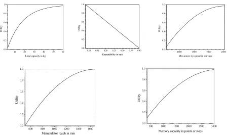
Using Eq. (22) and Eq. (23), the utility functions for different criteria for ASEA-IRB 60/2 robot are calculated, as given below.
Utility function for LC : u1(LC) = [(LC - 2.5)/(60 - 2.5)]0.5
Utility function for RE : u2(RE) = (0.4 - RE)/(0.4 - 0.08)
Utility function for MTS : u3(MTS) = [(MTS - 560)/(2540 - 560)]0.5
Utility function for MC : u4(MC) = [(MC - 350)/(3000 - 350)]0.5
Utility function for MR : u5(MR) = [(MR - 508)/(1676 - 508)]0.5
Table 12
Criteria-wise utility values for example 1
Robot LC RE MTS MC MR
ASEA-IRB 60/2 1 0 1 0.2379 0.6424
Cincinnati Milacrone T3-726 0.25876 0.78125 0.4799 1 0.6755
Cybotech V15 Electric Robot 0.273464 0.9375 0.7678 0.6588 1
with those of the past researchers, excellent consistency is observed for all the DEA-based models. Fig. 1 portrays the utility functions for all the five considered criteria.
10 20 30 40 50 60
0.0 0.2 0.4 0.6 0.8 1.0
U
til
ity
Load capacity in kg
0.10 0.15 0.20 0.25 0.30 0.35 0.40
0.0 0.2 0.4 0.6 0.8 1.0
U
tility
Repeatability in mm 1000 1500 2000 2500
0.0 0.2 0.4 0.6 0.8 1.0
U
til
ity
Maximum tip speed in mm/sec
600 800 1000 1200 1400 1600 0.0
0.2 0.4 0.6 0.8 1.0
U
til
ity
Manipulator reach in mm
500 1000 1500 2000 2500 3000 0.0
0.2 0.4 0.6 0.8 1.0
U
til
ity
Memory capacity in points or steps
Fig. 1. Utility functions for different criteria for example 1
Table 13
Weights of different criteria
Criteria LC RE MTS MC MR
wi 0.036 0.192 0.326 0.326 0.120
Table 14
Overall utility values and rankings of the robots
Robot Overall utility Rank Bhangale et al. (2004) Rao (2007) Chatterjee et al. (2010)
ASEA-IRB 60/2 0.5166 3 2 4 3
Cincinnati Milacrone T3-726 0.7228 2 3 2 2
Cybotech V15 Electric Robot 0.7749 1 1 1 1
4.2 Example 2
Using the normalized decision matrix of Table 16, the corresponding LP formulations for CCR, BCC, additive and cone-ratio models are developed for all the alternative robots. Tables 17, 18, 19 and 20 respectively show those mathematical formulations as involved in CCR, BCC, additive and cone-ratio models for robot 1. The LP problems are subsequently solved using LINDO software and the obtained results are given in Table 21.
Table 15
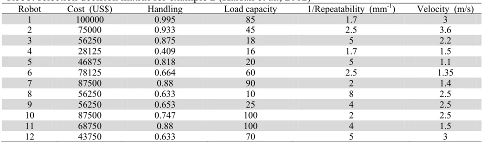
Robot selection decision matrix for example 2 (Karsak et al., 2012)
Robot Cost (US$) Handling Load capacity 1/Repeatability (mm-1) Velocity (m/s)
1 100000 0.995 85 1.7 3
2 75000 0.933 45 2.5 3.6
3 56250 0.875 18 5 2.2
4 28125 0.409 16 1.7 1.5
5 46875 0.818 20 5 1.1
6 78125 0.664 60 2.5 1.35
7 87500 0.88 90 2 1.4
8 56250 0.633 10 8 2.5
9 56250 0.653 25 4 2.5
10 87500 0.747 100 2 2.5
11 68750 0.88 100 4 1.5
12 43750 0.633 70 5 3
Table 16
Normalized decision matrix for example 2
Robot C HC LC R V
1 0.4220 0.3698 0.3898 0.1210 0.3749
2 0.3165 0.3468 0.2064 0.1780 0.4499
3 0.2374 0.3252 0.0825 0.3560 0.2749
4 0.1187 0.1520 0.0734 0.1210 0.1874
5 0.1978 0.3040 0.0917 0.3560 0.1375
6 0.3297 0.2468 0.2751 0.1780 0.1687
7 0.3692 0.3271 0.4127 0.1424 0.1749
8 0.2374 0.2353 0.0459 0.5696 0.3124
9 0.2374 0.2427 0.1146 0.2848 0.3124
10 0.3692 0.2777 0.4586 0.1424 0.3124
11 0.2901 0.3271 0.4586 0.2848 0.1874
12 0.1846 0.2353 0.3210 0.3560 0.3749
Table 17
Mathematical modeling of CCR model for robot 1 min g = 0.4220v1
subject to
-0.3698u1 - 0.3898u2 - 0.1210u3 - 0.3749u4 + 0.4220v1 ≥ 0 -0.3468u1 - 0.2064u2 - 0.1780u3 - 0.4499u4 + 0.3165v1 ≥ 0
-0.3252u1 - 0.0825u2 - 0.3560u3 - 0.2749u4 + 0.2374v1 ≥ 0 -0.1520u1 - 0.0734u2 - 0.1210u3 - 0.1874u4 + 0.1187v1 ≥ 0
-0.3040u1 - 0.0917u2 - 0.3560u3 - 0.1375u4 + 0.1978v1 ≥ 0 -0.2468u1 - 0.2751u2 - 0.1780u3 - 0.1687u4 + 0.3297v1 ≥ 0
-0.3271u1 - 0.4127u2 - 0.1424u3 - 0.1749u4 + 0.3692v1 ≥ 0 -0.2353u1 - 0.0459u2 - 0.5696u3 - 0.3124u4 + 0.2374v1 ≥ 0
-0.2427u1 - 0.1146u2 - 0.2848u3 - 0.3124u4 + 0.2374v1 ≥ 0 -0.2777u1 - 0.4586u2 - 0.1424u3 - 0.3124u4 + 0.3692v1 ≥ 0
-0.3271u1 - 0.4586u2 - 0.2848u3 - 0.1874u4 + 0.2901v1 ≥ 0 -0.2353u1 - 0.3210u2 - 0.3560u3 - 0.3749u4 + 0.1846v1 ≥ 0
0.3698u1 + 0.3898u2 + 0.1210u3 + 0.3749u4 = 1 Objective function value (g) is 1.5308.
Table 18
Mathematical modeling of BCC model for robot 1
Min G subject to
0.4220G - 0.4220λ1 - 0.3165λ2 - 0.2374λ3 - 0.1187λ4 - 0.1978λ5 - 0.3297λ6 - 0.3692λ7 - 0.2374λ8 - 0.2374λ9 - 0.3692λ10 - 0.2901λ11 - 0.1846λ12 ≥ 0
0.3698λ1 + 0.3468λ2 + 0.3252λ3 + 0.1520λ4 + 0.3040λ5 + 0.2468λ6 + 0.3271λ7 + 0.2353λ8 + 0.2427λ9 + 0.2777λ10 + 0.3271λ11 + 0.2353λ12 ≥ 0.3698
0.3898λ1 + 0.2064λ2 + 0.0825λ3 + 0.0734λ4 + 0.0917λ5 + 0.2751λ6 + 0.4127λ7 + 0.0459λ8 + 0.1146λ9 + 0.4586λ10 + 0.4586λ11 + 0.3210λ12 ≥ 0.3898
0.1210λ1 + 0.1780λ2 + 0.3560λ3 + 0.1210λ4 + 0.3560λ5 + 0.1780λ6 + 0.1424λ7 + 0.5696λ8 + 0.2848λ9 + 0.1424λ10 + 0.2848λ11 + 0.3560λ12 ≥ 0.1210
0.3749λ1 + 0.4499λ2 + 0.2749λ3 + 0.1874λ4 + 0.1375λ5 + 0.1687λ6 + 0.1749λ7 + 0.3124λ8 + 0.3124λ9 + 0.3124λ10 + 0.1874λ11 + 0.3749λ12 ≥ 0.3749
λ1 + λ2 + λ3 + λ4 + λ5 + λ6 + λ7 + λ8 + λ9 + λ10 + λ11+λ12 = 1
Table 19
Mathematical modeling of additive model for robot 1
Max Po = S1- + S1+ + S2++ S3++ S4+
subject to
0.4220λ1 + 0.3165λ2 + 0.2374λ3 + 0.1187λ4 + 0.1978λ5 + 0.3297λ6 + 0.3692λ7 + 0.2374λ8 + 0.2374λ9 + 0.3692λ10 + 0.2901λ11 + 0.1846λ12 + S1- = 0.4220
0.3698λ1 + 0.3468λ2 + 0.3252λ3 + 0.1520λ4 + 0.3040λ5+ 0.2468λ6 + 0.3271λ7 + 0.2353λ8 + 0.2427λ9 + 0.2777λ10 + 0.3271λ11 + 0.2353λ12 - S1+ = 0.3698
0.3898λ1 + 0.2064λ2 + 0.0825λ3 + 0.0734λ4 + 0.0917λ5 + 0.2751λ6 + 0.4127λ7 + 0.0459λ8 + 0.1146λ9 + 0.4586λ10 + 0.4586λ11 + 0.3210λ12 - S2+ = 0.3898
0.1210λ1 + 0.1780λ2 + 0.3560λ3 + 0.1210λ4 + 0.3560λ5 + 0.1780λ6 + 0.1424λ7 + 0.5696λ8 + 0.2848λ9 + 0.1424λ10 + 0.2848λ11 + 0.3560λ12 - S3+= 0.1210
0.3749λ1 + 0.4499λ2 + 0.2749λ3 + 0.1874λ4 + 0.1375λ5 + 0.1687λ6 + 0.1749λ7 + 0.3124λ8 + 0.3124λ9 + 0.3124λ10 + 0.1874λ11 + 0.3749λ12 - S4+ = 0.3749
λ1 + λ2 + λ3 + λ4 + λ5 + λ6 + λ7 + λ8 + λ9 + λ10 + λ11+ λ12 = 1
Objective function value (Po) is 0.
Table 20
Mathematical modeling of CRDEA model for robot 1 (for cone 1) Max 0.3698v1 + 0.3898v2 + 0.1210v3 + 0.3749v4
subject to
0.3698v1 + 0.3898v2 + 0.1210v3 + 0.3749v4 - 0.4220u1 ≤ 0 0.3468v1 + 0.2064v2 + 0.1780v3 + 0.4499v4 - 0.3165u1 ≤ 0
0.3252v1 + 0.0825v2 + 0.3560v3 + 0.2749v4 - 0.2374u1 ≤ 0 0.1520v1 + 0.0734v2 + 0.1210v3 + 0.1874v4 - 0.1187u1 ≤ 0
0.3040v1 + 0.0917v2 + 0.3560v3 + 0.1375v4 - 0.1978u1 ≤ 0 0.2468v1 + 0.2751v2 + 0.1780v3 + 0.1687v4 - 0.3297u1 ≤ 0
0.3271v1 + 0.4127v2 + 0.1424v3 + 0.1749v4 - 0.3692u1 ≤ 0 0.2353v1 + 0.0459v2 + 0.5696v3 + 0.3124v4 - 0.2374u1 ≤ 0
0.2427v1 + 0.1146v2 + 0.2848v3 + 0.3124v4 - 0.2374u1 ≤ 0 0.2777v1 + 0.4586v2 + 0.1424v3 + 0.3124v4 - 0.3692u1 ≤ 0
0.3271v1 + 0.4586v2 + 0.2848v3 + 0.1874v4 - 0.2901u1 ≤ 0 0.2353v1 + 0.3210v2 + 0.3560v3 + 0.3749v4 - 0.1846u1 ≤ 0
0.4220u1 = 1 v1 - v2 ≥ 0, v2 - v3 ≥ 0, v3 - v4 ≥ 0
Objective function value is 0.6532465.
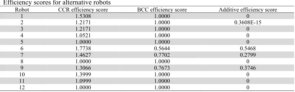
It is observed from Table 21 that robot alternatives 5, 8 and 12 emerge out as the efficient choices from CCR, BCC and additive models. It is also found that robot 12 is the most consistent efficiency scorer among all the 24 cones for CRDEA model.
Table 21
Efficiency scores for alternative robots
Robot CCR efficiency score BCC efficiency score Additive efficiency score
1 1.5308 1.0000 0
2 1.2171 1.0000 0.3608E-15
3 1.2171 1.0000 0
4 1.0521 1.0000 0
5 1.0000 1.0000 0
6 1.7738 0.5644 0.5468
7 1.4627 0.7702 0.2799
8 1.0000 1.0000 0
9 1.3066 0.7673 0.3746
10 1.3999 1.0000 0
11 1.0999 1.0000 0
12 1.0000 1.0000 0
Now, the weighted overall efficiency ranking method is applied to identify the most competent robot among the short-listed alternatives. Based on Eqns. (22)-(23), the computations of criteria-wise utility functions for robot 1 are shown as below.
Utility function for C : u1(C) = (100000-C)/(100000-28125)
Utility function for HC : u2(HC) = [(HC - 0.409)/(0.995 - 0.409)]0.5
Utility function for LC : u3(LC) = [(LC - 10)/(100 - 10)]0.5
Utility function for R : u4(R) = [(R - 1.7)/(8 - 1.7)]0.5
Utility function for V : u5(V) = [(V - 1.1)/(3.6 - 1.1)]0.5
Table 22
Weights of different criteria
Criteria C HC LC R V
wi 0.1071 0.1071 0.1624 0.3910 0.2323
The overall utility value for a robot is derived from the criteria weights and criteria-wise utility values, using the flowing expression:
Overall utility = w1(C)xu1(C) + w2(HC)xu2(HC) + w3(LC)xu3(LC) + w4(R)xu4(R) + w5(V)xu5(V)
= 0.1071u1(C) + 0.1071u2(HC) + 0.1624u3(LC) + 0.3910u4(R) + 0.2323u5(V)
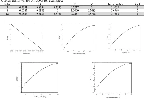
Table 23 shows the results of weighted overall efficiency ranking method. From this table, it is clear that the overall utility value of robot 12 is higher than that of the other two candidate robots. So, the best choice of alternative is robot 12. Braglia and Gabbrielli (2000) and Karsak et al. (2012) also identified robot 12 as the best selection. Hence, from the derived results, it is found that the two-phase method employing DEA models is a consistent and effective technique for robot selection decision-making. Fig. 2 shows the utility functions for all the five criteria as involved in this example.
Table 23
Overall utility values of robots for example 2
Robot C HC LC R V Overall utility Rank
5 0.7391 0.8354 0.3333 0.7237 0 0.5058 3
8 0.6087 0.6183 0 1.0000 0.7483 0.6963 2
12 0.7826 0.6183 0.8165 0.7237 0.8718 0.7682 1
30000 40000 50000 60000 70000 80000 90000 100000 0.0
0.2 0.4 0.6 0.8 1.0
Ut
ility
Cost (US$)
0.5 0.6 0.7 0.8 0.9
0.0 0.2 0.4 0.6 0.8 1.0
U
tilit
y
Handling coefficient
1.5 2.0 2.5 3.0 3.5
0.0 0.2 0.4 0.6 0.8 1.0
Uti
lit
y
Velocity (m/s)
20 40 60 80 100
0.0 0.2 0.4 0.6 0.8 1.0
U
tili
ty
Load capacity (Kg)
2 3 4 5 6 7 8
0.0 0.2 0.4 0.6 0.8 1.0
U
tility
1/Repeatability (mm-1
)
Fig. 2. Utility functions for different criteria for example 2
5. Conclusions
combined approach helps to determine the most appropriate robot by eliminating the unsuitable ones. The CCR, BCC and additive models usually provide multiple choices as the efficient alternative solutions, whereas, CRDEA model provides a single unique solution. But in a general case, CRDEA model may also identify multiple efficient alternatives to be considered. The main disadvantage of CRDEA model is that it is mathematically rigorous and not easily comprehensible. Thus, the two-phase approach combining any of the CCR, BCC and additive models of DEA and weighted overall efficiency ranking method can be effectively employed to any type of complex decision-making problems, involving selection of the most appropriate alternative with conflicting performance measures.
References
Alinezhad, A., Makui, A., Mavi, R.K., & Zohrehbandian, M. (2011). An MCDM-DEA approach for technology selection. Journal of Industrial Engineering: International, 7(12), 32-38.
Athawale, V.M., & Chakraborty, S. (2011). A comparative study on the ranking performance of some multi-criteria decision-making methods for industrial robot selection. International Journal of
Industrial Engineering Computations, 2(4), 831-850.
Athawale, V.M., Chatterjee, P., & Chakraborty, S. (2012). Selection of industrial robots using compromise ranking method. International Journal of Industrial and Systems Engineering, 11(1/2), 3-15.
Banker, R.D., Charnes, A., & Cooper, W.W. (1984). Some models for estimating technical and scale efficiencies in data envelopment analysis. Management Science, 30(9), 1078-1092.
Bhangale, P.P., Agrawal, V.P., & Saha, S.K. (2004). Attribute based specification, comparison and selection of a robot. Mechanism and Machine Theory, 39(12), 1345-1366.
Bhattacharya, A., Sarkar, B., & Mukherjee, S.K. (2005). Integrating AHP with QFD for robot selection under requirement perspective. International Journal of Production Research, 43(17), 3671-3685. Braglia, M., & Petroni, A. (1999). Evaluating and selecting investments in industrial robots.
International Journal of Production Research, 37(18), 4157-4178.
Braglia, M., & Gabbrielli, R. (2000). Dimensional analysis for investment selection in industrial robots.
International Journal of Production Research, 38(18), 4843-4848.
Brockett, P.L., Charnes, A., Cooper, W.W., Huang, Z.M., & Sun, D.B., (1997). Data transformations in DEA cone ratio envelopment approaches for monitoring bank performances. European Journal of
Operational Research, 98(2), 250-268.
Charnes, A., Cooper, W.W., & Rhodes, E. (1978). Measuring the efficiency of decision making units.
European Journal of Operational Research, 2(6), 429-444.
Charnes, A., Cooper, W.W., Golany, B., Seiford, L.M., & Stutz, J. (1985). Foundations of data
envelopment analysis and Pareto-Koopmans empirical production functions. Journal of
Econometrics, 30(1-2), 91-107.
Charnes, A., Cooper, W.W., Huang, Z.M., & Sun, D.B. (1990). Polyhedral cone-ratio DEA models with an illustrative application to large commercial banks. Journal of Econometrics, 46(1-2), 73-91. Chatterjee, P., Athawale, V.M., & Chakraborty, S. (2010). Selection of industrial robots using
compromise ranking and outranking methods. Robotics and Computer-Integrated Manufacturing, 26(5), 483-489.
Chu, T-C., & Lin, Y-C. (2003). Fuzzy TOPSIS method for robot selection. International Journal of
Advanced Manufacturing Technology, 21(4), 284-290.
Cook, W.D., & Seiford, L.M. (2009), Data envelopment analysis (DEA) - Thirty years on. European
Journal of Operational Research, 192(1), 1-17.
Cooper, W.W., Lawrence, M.S., & Zhu, J. (2011). Handbook on data envelopment analysis.
International Series in Operations Research & Management Science, Springer, 164, 1-40
Devi, K. (2011), Extension of VIKOR method in intuitionistic fuzzy environment for robot selection.
Goh, C-H., Tung, Y-C.A., & Cheng, C-H. (1996). A revised weighted sum decision model or robot selection. Computers & Industrial Engineering, 30(2), 193-199.
Goh, C-H. (1997). Analytic hierarchy process for robot selection. Journal of Manufacturing Systems, 16(5), 381-386.
Kahraman, C., Çevik, S., Ates, N.Y., & Gülbay, M. (2007). Fuzzy multi-criteria evaluation of industrial robotic systems. Computers & Industrial Engineering, 52(4), 414-433.
Karsak, E.E. (1998). A two-phase robot selection procedure. Production Planning & Control, 9(7), 675-684.
Karsak, E.E., & Ahiska, S.S. (2005). Practical common weight multi-criteria decision-making approach with an improved discriminating power for technology selection. International Journal of
Production Research, 43(8), 1537-1554.
Karsak, E.E. (2008). Robot selection using an integrated approach based on quality function deployment and fuzzy regression. International Journal of Production Research, 46(3), 723-738. Karsak, E.E., Sener, Z., & Dursun, M. (2012). Robot selection using a fuzzy regression-based
decision-making approach. International Journal of Production Research, 50(23), 6826-6834.
Khouja, M. (1995). The use of data envelopment analysis for technology selection. Computers and
Industrial Engineering, 28(1), 123-132.
Khouja, M., & Booth, D.E. (1995). Fuzzy clustering procedure for evaluation and selection of industrial robots. Journal of Manufacturing Systems, 14(4), 244-251.
Khouja, M.J., (1999). An options view of robot performance parameters in a dynamic environment.
International Journal of Production Research, 37(6), 1243-1257.
Koulouriotis, D.E., & Ketipi, M.K. (2011). A fuzzy digraph method for robot evaluation and selection.
Expert Systems with Applications, 38(9), 11901-11910.
Kuah, C.T., Wong, K.Y., & Behrouzi, F. (2010). A review on data envelopment analysis (DEA). Proc.
of 4th Asia International Conference on Mathematical/Analytical Modelling and Computer
Simulation, 168-173.
Kumar, R., & Garg, R.K. (2010). Optimal selection of robots by using distance based approach method.
Robotics and Computer-Integrated Manufacturing, 26(5), 500-506.
Liang, G-S., & Wang, M-J.J. (1993). A fuzzy multi-criteria decision-making approach for robot selection. Robotics and Computer-Integrated Manufacturing, 10(4), 267-274.
Parkan C. and Wu M-L. (1999) ‘Decision-making and performance measurement models with applications to robot selection’, Computers & Industrial Engineering, Vol. 36(3), pp. 503-523. Ramanathan, R. (2003). An introduction to data envelopment analysis: A tool for performance
measurement. Sage Publications: New Delhi.
Rao, R.V., & Padmanabhan, K.K. (2006). Selection, identification and comparison of industrial robots using digraph and matrix methods. Robotics and Computer-Integrated Manufacturing, 22(4), 373-383.
Rao, R.V. (2007). Decision making in the manufacturing environment using graph theory and fuzzy multiple attribute decision making methods. Springer-Verlag: London.
Rao, R.V., Patel, B.K., & Parnichkun, M. (2011). Industrial robot selection using a novel decision
making method considering objective and subjective preferences. Robotics and Autonomous
Systems, 59(6), 367-375.
Roghanian, E., & Foroughi, A. (2010). An empirical study of Iranian regional airports using robust data envelopment analysis. International Journal of Industrial Engineering Computations, 1(1), 65-72. Shih, H-S. (2008). Incremental analysis for MCDM with an application to group TOPSIS. European
Journal of Operational Research, 186(2), 720-734.
Sun, C., & Gui, X. (2011). Data envelopment analysis: surveys. Proc. of International Conference on
Management and Service Science, China, 1-4.
Talluri, S., & Yoon, K.P. (2000). A cone-ratio DEA approach for AMT justification. International