Patron: Her Majesty The Queen Rothamsted Research Harpenden, Herts, AL5 2JQ
Telephone: +44 (0)1582 763133 Web: http://www.rothamsted.ac.uk/
Rothamsted Research is a Company Limited by Guarantee Registered Office: as above. Registered in England No. 2393175.
Rothamsted Repository Download
A - Papers appearing in refereed journals
Oakey, H., Cullis, B., Thompson, R., Comadran, J., Halpin, C. and
Waugh, R. 2016. Genomic Selection in Multi-environment Crop Trials.
G3. 6 (5), pp. 1313-1326.
The publisher's version can be accessed at:
•
https://dx.doi.org/10.1534/g3.116.027524
The output can be accessed at:
https://repository.rothamsted.ac.uk/item/8v35q
.
© 11 March 2016. Licensed under the Creative Commons CC BY.
GENOMIC SELECTION
Genomic Selection in Multi-environment Crop Trials
Helena Oakey,*,1Brian Cullis,†Robin Thompson,§Jordi Comadran,**,2Claire Halpin,*,3 and Robbie Waugh*,**,3
*Division of Plant Sciences, School of Life Sciences, University of Dundee at The James Hutton Institute, and **Department of Cell and Molecular Sciences, James Hutton Institute, Invergowrie, Dundee DD2 5DA, Scotland, UK,
†National Institute for Applied Statistics Research Australia, University of Wollongong, NSW, 2522, Australia, and §Rothamsted Research, Harpenden, Hertfordshire AL5 3JQ, UK
ORCID ID: 0000-0002-1808-8130 (C.H.)
ABSTRACT Genomic selection in crop breeding introduces modeling challenges not found in animal studies. These include the need to accommodate replicate plants for each line, consider spatial variation infield trials, address line by environment interactions, and capture nonadditive effects. Here, we propose aflexible single-stage genomic selection approach that resolves these issues. Our linear mixed model incorporates spatial variation through environment-specific terms, and also randomization-based design terms. It considers marker, and marker by environment interactions using ridge regression best linear unbiased prediction to extend genomic selection to multiple environments. Since the approach uses the raw data from line replicates, the line genetic variation is partitioned into marker and nonmarker residual genetic variation (i.e., additive and nonadditive effects). This results in a more precise estimate of marker genetic effects. Using barley height data from trials, in 2 different years, of up to 477 cultivars, we demonstrate that our new genomic selection model improves predictions compared to current models. Analyzing single trials revealed improvements in predictive ability of up to 5.7%. For the multiple environment trial (MET) model, combining both year trials improved predictive ability up to 11.4% compared to a single environment analysis. Benefits were significant even when fewer markers were used. Compared to a single-year standard model run with 3490 markers, our partitioned MET model achieved the same predictive ability using between 500 and 1000 markers depending on the trial. Our approach can be used to increase accuracy and confidence in the selection of the best lines for breeding and/or, to reduce costs by using fewer markers.
KEYWORDS
multi-environment trial
genomic selection random ridge
regression GEBV barley GenPred shared data
resource
Whole genome prediction (WGP) uses genotypic information in the form of molecular genetic markers to predict individual phenotypic performance, and has utility in livestock and crop breeding. For a
particular population, WGP associates a phenotypic value with each molecular marker allele, which is consequently known as a marker effect. The sum of the marker effects (which relate to the alleles present in an individual’s genotype) is a predictor of their phenotypic performance, and is known as a genomic estimated breeding value (GEBV). In‘ Ge-nomic Selection’(GS), the GEBV is used to select the best parents for breeding, or to predict the performance of progeny using only genotyp-ing data without the need for phenotypic screengenotyp-ing. In order to derive GEBVs for prediction, an initial ‘training population’is phenotyped and genotyped to estimate marker effects. GEBVs can then be calcu-lated for individuals descended from, or recalcu-lated to, the training pop-ulation (a‘validation population’) that have not been phenotyped, but for which genotypic information is available. This saves both time and the costs associated with phenotyping in a breeding program. Since GS uses all genetic markers to calculate the GEBV, it potentially captures all of the loci that influence a trait. This distinguishes GS from more traditional marker assisted selection (MAS), where a few diagnostic markers are used to follow the inheritance of specific loci influencing
Copyright © 2016 Oakeyet al.
doi: 10.1534/g3.116.027524
Manuscript received October 3, 2015; accepted for publication March 5, 2016; published Early Online March 11, 2016.
This is an open-access article distributed under the terms of the Creative Commons Attribution 4.0 International License (http://creativecommons.org/ licenses/by/4.0/), which permits unrestricted use, distribution, and reproduction in any medium, provided the original work is properly cited.
Supplemental material is available online atwww.g3journal.org/lookup/suppl/ doi:10.1534/g3.116.027524/-/DC1
1Present address: Biomathematics and Statistics Scotland (BioSS), The James
Hutton Institute, Dundee, DD2 5DA Scotland, UK.
2Present address: Limagrain, Biopôle Clermont-Limagne, Rue Henri Mondor,
63360 Saint-Beauzire, France.
3Corresponding authors: Division of Plant Sciences, School of Life Sciences,
a trait, and marker assisted recurrent selection (MARS), where only a subset of significant markers are used to select for quantitative trait loci (QTL) in a given population. The potential of GS to accelerate crop improvement due to shorter generation times and the avoidance of phenotypic evaluation has been established (Janninket al.2010), and shown to outperform MAS (Heffneret al.2010) and MARS (Massman
et al.2013).
Since 2001, when Meuwissenet al.(2001) compared least square, ridge regression best linear unbiased prediction (RR-BLUP) and two Bayesian approaches (BayesA and BayesB) for GS in animal breeding, there has been an increase in the number of methods available (Wang
et al. 2012; de los Camposet al. 2013; Desta and Ortiz 2014), and widespread uptake, particularly in dairy cattle breeding, where official GEBVs are published (http://www.interbull.org). These GS methods, however, differ in their predictive ability (de los Camposet al.2013) and suitability for specific applications. Crop populations may require different GS methods to those of animals due to the potential presence of extensive linkage disequilibrium (LD), population substructure, and agronomic performance traits which are often influenced by many QTL of small effect (Wimmeret al.2013). In a simulated data set based on actual marker data from barley, RR-BLUP was found to be more accurate than BayesB (Zhonget al.2009), and has been recommended for crop improvement applications (Heslotet al.2012). Wimmeret al.
(2013) compared the performance of four commonly used methods; RR-BLUP and BayesB (Meuwissen et al. 2001), LASSO (Tibshirani 1996), and the elastic net (Zou and Hastie 2005). They also found good performance with BLUP, and recommended its use in crops. RR-BLUP has the advantage over Bayesian approaches of being easily implemented and quick.
Despite these advances, GS is only starting to be adopted in crop breeding. Some of the reluctance to adopt GS may be due to the additional modeling challenges of crop improvement scenarios. Suitable models need to accommodate data from replicate plants of the same line, the influence of spatial variation in thefield, and potentially different
‘environments’if the crop is trialed in several locations or multiple years. These variables introduce significant genotype by environment interactions (G · E) and new methods are needed that consider G · E effects, as well as nonadditive effects, and the crop-specific (in)breeding cycle (Jonas and De Koning 2013).
The reasons for considering spatial variation in crop breeding activities are obvious. Every trial (or environment) will have considerable sources of nongenetic variation such that even the position of a line in the
field will impact its phenotypic response. Allowing for spatial variation through appropriate trial design and analysis will ensure that more accurate genetic effects are revealed (Gilmouret al.1997). In GS, this is also true; the accuracy of genomic prediction in RR-BLUP is improved after adjusting for spatial variation using moving-means as a covariate in the model (Ladoet al.2013).
Similarly, consideration should be paid to the fact that crop lines are often assessed in a multi environment trial (MET), i.e., in different geographic locations, seasons, or years, in order to determine perfor-mance stability across environments (i.e., G · E). In GS, G · E is an important component of genetic variability (Crossaet al.2010, 2011). A MET in a GS context is therefore an important extension as it allows the examination of marker by environment (M · E) interactions, and, in particular, the identification of markers whose effects are stable across environments (trials), as well as those that are environment-specific. As RR-BLUP involvesfitting a linear mixed model, the incorporation of a MET extension is straightforward, and improvements in prediction when using two stage approaches to MET analysis have already been shown (Burguenoet al.2012; Guoet al.2013).
Capturing nonadditive effects in genomic selection is more compli-cated because the genomic relationship matrix described by the markers and used in RR-BLUP captures not only additive genetic relationships at QTL but also LD and cosegregation information (Habieret al.2013). A
first step toward modeling nonadditive effects in GS is to include ped-igree information that captures a polygenic effect. Pedped-igree information included in a BayesB model in animal GS marginally improved the accuracy of selection, and reduced bias, which is important when marker effect estimates are used over multiple generations (Solberg
et al.2009). A small improvement in crops has also been shown (Crossa
et al.2010). Burguenoet al.(2012) explored the inclusion of pedigree information in RR-BLUP MET models, and found that it improved prediction accuracy for individual lines in some circumstances, but not others. However, compared to use of pedigree, inclusion of both addi-tive and nonaddiaddi-tive marker-based, or realized genomic relationship matrices further improves prediction of breeding values (Munozet al.
(2014).
Most methods of crop GS use a two-stage analysis. First, data from individual replicated plants or plots are used to derive the line means. This allows software already developed for animal studies, which cannot handle replicates, to use the means for RR-BLUP in the second stage. However, a two-stage approach biases marker effects, and induces heterogeneous residual variances and residual correlations that are not completely eliminated by a weighted analysis (de los Campos
et al.2013). A single-stage approach that uses individual plant or plot data, includes replication, and accounts for spatial variation and ran-domization-based terms (e.g., blocking factors), would be preferable because it would not have the difficulties associated with a two-stage approach. Incorporating data from individual plant or plot replicates would have additional advantages for GS. Markers may not capture all the genetic variation contributing to the phenotype, particularly if the number of markers used for prediction is low. Including replicates allows the total genetic effect due to lines to be partitioned into the genetic effect due to markers, and a residual genetic effect not captured by markers, which will include nonadditive genetic effects. This ap-proach is possible without the need for pedigree information (which is not always available), would be more encompassing than a polygenic effect, and would not require the calculation of additional matrices that can induce dependency between variance components. In addition, separating out the nonadditive genetic effects from the model residual variance should increase the accuracy and predictive ability of the additive genetic effects compared to two-stage analyses.
In this paper, we propose such a single-stage approach to the analysis of multi-environment data byfitting a single linear mixed model that extends single trial RR-BLUP analysis. Marker and M · E interactions are incorporated as terms in the model, and form the basis for the analysis of METs. In this GS approach, the marker and M · E in-teraction terms are assumed to be random using RR-BLUP, and the approach extends RR-BLUP analysis by partitioning the term for ge-netic variation into marker and nonmarker (or residual gege-netic) vari-ation using raw data from individual replicates, rather than line means. Wefirst outline the proposed method that we refer to aspartitioned
RR-BLUP for MET, and then illustrate its use on a real data set with appropriate comparisons to nonpartitioned, orstandard, models and single trial RR-BLUP analysis, both within a single-stage approach.
MATERIALS AND METHODS
Description of motivating example
cultivated barley. During two consecutive years (2010 and 2011; referred to also as trials), spring barley lines were grown in pots, in thefield, within a polythene tunnel, with each pot containing one plant (from one line). In each trial, the pots were arranged in a spatial row-column design withfive replicate blocks, where the replicate blocks correspond to bi-ological replicates. In the 2010 trial, 648 lines were planted with pots arranged in 405 columns by eight rows, with each replicate block con-sisting of 81 columns by eight rows. In the 2011 trial, 856 lines were planted with pots arranged in 535 columns by eight rows, with each replicate block containing 107 columns (see Oakeyet al.2013 for further details). There were 639 lines common to both trial years. The lines were predominantly European elite cultivars of two-row spring barley. At full maturity, the height of each plant was measured in centimeters from the base of the plant to the top of the main stem. The software CycDesigN 4.0 (VSN International) was used to generate the design each trial year. A set of 7864 high-confidence, gene-based single nucleotide poly-morphism (SNP) markers, incorporated into a single Illumina iSelect assay (Illumina Inc.), was used to genotype DNA extracted from 477 lines (Comadranet al.2012), including 459 lines grown across both years, one line from 2010 only, and 17 lines from 2011 only. Non-polymorphic SNPs, and SNPs with more than 20% missing values, were removed. For each marker, individuals were coded as 0 (homozy-gous minor allele), or 2 (homozy(homozy-gous major allele). The population consists of lines that are derived via single seed descent and should be homozygous; a heterozygous marker within a particular individual suggests that there is an error with the calling of the marker, thus these heterozygous markers were coded as missing. Missing values were imputed using the R package impute (Hastieet al.2014). Markers that were heterozygous and failed to converge to either 0 or 2 after several iterations were discarded, because this suggests the marker itself may not be appropriate for use. This resulted in a set of 4654 homozygous markers with a minimum minor allele frequency of.5% and map positions available for analysis. Thefinal set of 3490 markers used in the analysis was a subset of the 4654 markers, and had no two markers identical in terms of their qualitative coding across the lines. Pedigree information on the lines was unavailable. The phenotypic and geno-typic data are available in Supplemental Material,File S2.
General form of the new model for whole genome prediction
A general form of the new model is now presented. This is a single linear mixed model that incorporates marker and M · E interactions as terms in the model with appropriate variance-covariance structures to allow for correlation between trials. In this new approach, the genetic variation is partitioned into marker and nonmarker (or residual) var-iation through the inclusion of all raw data in the model. In addition, spatial trends and design and randomized factors can be easily incor-porated in the model. The new model is referred to as thepartitioned
RR-BLUP for MET. We use the term‘trial’to denote different envi-ronments, which for our example data set represents different years.
Consider a data set consisting ofvlines andstrials. The new mixed model for whole genome prediction can be developed as follows
y¼XtþZggþZuuþe (1) where yðn·1Þ¼ ðyT
1;. . .;yTs Þ T
is the vector of response across each of thestrials, yðnt·1Þ
t is the vector of response for trialtand
n¼P
s
t¼1
nt, wherent is the number of observations (pots) in trialt,
t is a vector offixed terms, consisting of an overall mean perfor-mance for each trial, as well as trial specific global or extraneous
spatial terms, for example, linear row or linear column effects, and
Xis the associated design matrix,gðvs·1Þis the vector of random line
effects of thevlines in each of thestrials with design matrixZg, and
has the general form,
g¼ ðIs5MÞumþue (2)
Mis the (v·pÞmatrix ofvlines bypSNP markers,Isis the (s·sÞidentity
matrix,uðmps·1Þis the vector ofprandom SNP marker effects in each of
strials anduðevs·1Þis the vector ofvrandom residual genetic effects in each
ofstrials, and represents line variation (and therefore genetic variation) that has not been accounted for by the markers;5is the kronecker product.
Letumtake a general form
um¼Lmfmþdm (3) Where Lm is a (ps·pkÞ matrix, fðmpk·1Þ is a vector with
var(fm) =Gm5Ip, where Gm is a (k·kÞ matrix for k factors, dðmps·1Þis a vector with varðdm) =Cm5IpwhereCmis the (s·sÞ
marker genetic variance matrix across trials. Letuealso take a general form
ue¼Lefeþde (4) Where Le is (vs·vlÞ matrix, fðevl·1Þ is a vector with
var(fe) = Ge5Iv where Ge is a (l·lÞ matrix for l factors, dðevs·1Þis a vector with varðde) = Ce5Iv whereCe is the (s·sÞ
residual genetic variance matrix across trials.
Thus withstrials, the genetic variance matricesCmandCeare both
(s·sÞmatrices, each withsðsþ1Þ
2 parameters to be estimated. LetLm¼Lm15Ip andLe¼Le15Iv, whereLm1 andLe1 are
(s·kÞand (s·lÞmatrices of k andl factor loadings for each trial, respectively
then
varðumÞ ¼
Lm1GmLTm1þCm
5Ip
and
varðueÞ ¼
Le1GeLTe1þCe
5Iv
The vectoruðb·1Þconsists of sub vectorsuðbi·1Þ
i , where the subvector
ui corresponds to theith random term. The corresponding design
matrix Zðub·1Þis partitioned conformably as½Zu1. . .Zub. The
sub-vectors are assumed mutually independent with varianceu2 iIbi. The
subvectors include random terms for describing spatial trends in in-dividual trials, such as random row, random column, or spline terms. The residual vector ehas variance R¼4s
t¼1Rt, a block diagonal
matrix ofsblocks,Rt¼u2tInt.
In crops, the modeling of spatial trends in field trials is crucial (Gilmouret al.1997), and the model above enables the addition of these trends where necessary. Furthermore, trial-specific design or random-ization-based terms such as blocking factors can also be included in the model (Culliset al.2006).
Thus the line termgreflects the total genetic variation partitioned into additive variation as described by the markers and residual genetic or nonadditive variation, thefixedt, randomuand residualeterms reflect the design and conduct of the trials, and as such provide the underlying structure for nongenetic variation.
There are two special cases ofg. Aphenotypicmodel can befitted by lettingg¼ue, so that theummarker term is omitted, andgrepresents
total genetic variation (assuming unrelated lines) as described by the phenotypic information. AstandardRR-BLUP model for GS can be
fitted by lettingg¼ ðIs5MÞum, so thatue, the residual genetic term, is
omitted; here,grepresents additive genetic variation as described by the markers. Thestandardmodel reflects the most common current prac-tice in GS, where only the markers are included in the model. These two additional models will be used as comparators to the newpartitioned
model.
Special cases of the general form of um:From the general form ofum
(Equation 3), special cases ofs, the number of trials, andk, the number of factors, can be considered. By varyings, single and multiple envi-ronment trials are encompassed, and by varyingkdifferent structures for the variance-covariance matrix ofumcan be considered (Table 1).
Varyingkenables an appropriate form of the varðumÞto be established
to describe the correlation structure between trials, and may vary depending on the data set. A similar table of special cases of the form ofue(Equation 4) can also be constructed ifl¼k,e¼mand
v¼p.
For a single trialuðmp·1Þ¼dðmp·1Þis a main marker term, with
varðumÞ ¼u2mIp. Models for multiple environment trials are now
discussed.
The simplest model for more than one trial is the diagonal (DIAG) model, whereuðmsp·1Þ¼dðmsp·1Þis a main marker term in
each of the trials. The varðumÞ ¼Cm5Ip, where Cm has
off-diagonals for all trials assumed zero. The DIAG model therefore assumes a separate marker variance for each trial, and no marker covariance between trials, and is equivalent to fitting each trial separately.
In the compound symmetry (CS) model,fðp·1Þ
m is a main term for
markers, anddðmps·1Þis an interaction term for the markers and trials.
All trials have the same marker variance, and all pairs of trials have the same marker covariance, so that the varðumÞ ¼ ðu2mJsþCmÞ5Ip
whereJsis (s·sÞmatrix of ones andCm¼u2meIs.
For the Culliset al.(1998) (CS+DIAG) model,fðmp·1Þis a main
marker term, anddðmps·1Þis a term for the interaction of the markers
and trials. This model assumes the same marker covariance for pairs of trials, and a separate marker variance for each trial. Thus, the form of varðumÞis the same in the CS and (CS+DIAG) models; however, in the
latter,Cm¼4st¼1u2mt. In this model, the covariance between pairs of
trials is assumed to be not greater than the variance of the individual trials.
An unstructured (US) model allows different marker variances and covariances between trials, so thatuðmsp·1Þ¼dðmsp·1Þis an interaction
term of the markers and trials, and no main marker effect isfitted. The varðumÞ ¼Cm5Ip, whereCmhas diagonal elements that are
the marker variances for the individual trials, and off-diagonal element that are the marker covariance between trials. As the number of trials increases, the US model becomes over parameterized, making it diffi -cult tofit.
Multiplicative models have been shown to work well in practice in MET analysis (Smith et al.2005), and are viable alternatives to the unstructured model. In fact, Kellyet al.(2007) found that the factor analytic model withkfactors (FAk) of Smithet al.(2001) was preferred over an unstructured model because it improved the predictive accu-racy of the line empirical BLUPs.
In a GS situation, a factor analytic model with a main marker term andkfactors (FAMk) may be more appropriate than a FAk
model that excludes this term. This is because a main marker term
represents QTL that are common and stable across trials (in the absence of an interaction between trials and markers) and the marker · trial term will give information on QTL that are trial or environment specific.
Smithet al.(2001) showed that a FAMkmodel is equivalent to a factor analytic model with (k+1) factors, where the first set of loadings are constrained to be equal. For a FAMk model, we letfT
m¼ ðfT0;fTÞ, where u0¼umf0, with varðu0Þ ¼u2mIp,fðsk·1Þ
is a vector of line scores with varðfÞ ¼Ik5Ip, then
varðumÞ ¼ ðu2mJsþLfLTf þCmÞ5Ip, whereLf is a (s·kÞmatrix
of loadings, andCmis a diagonal matrix with the diagonal elements
referred to as specific variances. The approach of including a main marker term is in contrast to a phenotypic model for estimating genotypic values, where, in cropfield trials, the main line term is usually excluded. Notice whenk = 0, the FAM0model is equivalent to the CS+DIAG model. The special cases of the general form ofum
shown in Table 1, can befitted in each of the three models, pheno-typic, standard, and partitioned, which reflect different forms of
g(Equation 2).
Computational efficiency: If the number of markers exceeds the number of individuals, we canfit
ug¼ ðIs5MÞum
The analysis will now be dependent on the number of lines rather than on the number of markers, and therefore will reduce the dimension-ality of the model, making it more computationally efficient (Stranden and Garrick 2009).
The estimation of variance parameters is by residual maximum likelihood (REML). Given estimates of the variance components, em-pirical best linear unbiased predictors (E-BLUPs) were obtained for random terms from the mixed model equations as
~
um¼
Is5MT
MMT21~u
g (5)
where~ugis the vector of genomic breeding values in each trial.
Here, we use MMTas in Piephoet al.(2012), whereMMT
repre-sents a realized genomic relationship matrix. Meuwissenet al.(2001) usedMMT=p, wherepis the number of marker (locations), and Habier
et al. (2007) usedMMT=2P
q
pqð12pqÞ, wherepq is the allele
fre-quency at marker locusq. Omission of the scalar term will not affect the conclusions of the analysis.
IfðMMTÞ21is of full rank, then var
ug
um
¼Gf5
MMT M
MT I
p
forGf ¼Lm1GmLTm1þCm
Thus, if
ug¼ ðIs5MÞum¼ ðIs5MÞLmfmþ ðIs5MÞdm¼ufþud
Then, the E-BLUPs obtained from the mixed model equations are
Lm~fm¼
Is5MT
MMT21~u
f (6)
and
~ dm¼
Is5MTMMT21u~
IfðMMTÞ21is of full rank, then
var
uf
Lmfm
¼Lm1GmLTm15
MMT M
MT I
p and var
ud
dm
¼Cm5
MMT M
MT I p
For our data set, the number of markers exceeds the number of individuals, therefore thestandardandpartitionedmodels werefitted using the computationally efficient approach. All models werefitted in ASReml v3.0-1 (Butleret al.2009) for R v3.2.0 (R Core Team 2015). Instructions for completing all the analysis shown in the paper can be found inFile S1along with supporting data (File S2) and R scripts (File S3,File S4,File S5,File S6,File S7,File S8,File S9,File S10,File S11,File S12,File S13,File S14,File S15,File S16,File S17,File S18, andFile S19).
Heritability
The calculation of the generalized heritability in complex linear mixed models is not straightforward (Culliset al.2006). Here, the generalized heritability for each trial is calculated from the phenotypic model (whereg¼ue) as 12
a
2u2gt
whereais the average pairwise prediction
error variance of line effects, andu2gtis the genetic variance of trial t
(Culliset al.2006). The R code for calculating the heritability is inFile S19.
Cross-validation
Initially, thephenotypic,standard, andpartitionedmodels werefitted using thefulldata set to enable the most appropriate MET form ofum
(Table 1), the term representing marker or additive variation, andue,
the term representing nonadditive or residual genetic variance, to be established for use in the cross-validation. A single trial analysis was also investigated in the cross-validation represented by the DIAG form. We generally denote thephenotypic,standard, andpartitionedmodels with specific forms ofumas EFORM, SFORM, and PFORM, respectively
[where FORM is either DIAG, US, CS, CS+DIAG, or FAMk(Table 1)]. To establish which MET form ofumis superior, and to undertake
initial comparisons between the three models, the Akaike information criteria (AIC) (Akaike 1974), or log-likelihood ratio test (if the models were nested), were used. For example, the phenotypicandstandard
model are nested within thepartitionedmodel when the form ofum
is the same, and can be compared using the log-likelihood ratio test. However, models with different forms forum need to be compared
using the AIC. The AIC was calculated as twice the number of random parameters minus twice the log-likelihood (the number of
fixed parameters was ignored in this calculation as this was constant over the models). For the AIC, lower values indicate superior models. Once the form ofumfor the MET analyses has been established, the
cross-validations could proceed.
The cross-validation involved randomly dividing the lines in the data set (as evenly as possible) into 10 groups, which were used across the single and MET analyses so that consistency and comparability was maintained as much as possible (Table 2).
Three different cross-validations were examined, and were defined by the number of groups in the validation and training sets. These were CV10, CV20, and CV40, where approximately 10, 20, and 40% of lines, respectively, were included in the validation set (Table 3), with the remaining lines used as the training set. Iteration across all combina-tions was investigated. For example, for the CV20 cross-validation, two groups (the validation set) were omitted in any one iteration. To cover the possible combinations of two of the 10 groups, a total of 45 itera-tions were necessary. The R scripts with details of the random division of the data and group combinations for CV10, CV20, and CV40 are in
File S3,File S4, andFile S5, respectively.
Using the training set, marker effects were obtained under each model (standard and partitioned), each cross-validation (CV10, CV20, and CV40), and each scenario (single trial 2010, single trial 2011, and MET). The marker effects (Equation 6 and Equation 7) were used to predict the GEBVs of the lines in the validation set. The DIAG form ofumanduewas
used to generate marker effects equivalent to analyzing each trial separately, with each trial having one set of marker effects. For the MET analyses of both trials, different forms ofumandue(Table 1) were initially investigated
as described previously, with the most appropriate forms used in the cross-validation. For the CS, CS+DIAG, and FAM1forms ofumandue, there
were three sets of marker effects. These were: the main marker effects, representing markers that are stable across both trials, and marker effects from each trial, which represent the additional marker by trial interaction. A total marker effect for each trial was obtained by adding the main marker effect to the marker by trial interaction effect. For completeness, the US form, which produces only total marker effects for each trial, was also initially investigated, although, as we are interested in MET models with main marker effects, the cross-validation focused on the most appropriate of the CS, CS+DIAG, and FAM1forms.
In simulations, the true breeding value is known, and the GEBV calculated in the lines of the validation set can be compared to the true breeding values to determine the predictive ability and the accuracy and precision of the GEBV. As real data were used here, the true breeding value was unknown. In the absence of pedigree information, the genotypic values (GV) of the lines in the validation set were used as the comparator. These were calculated from aphenotypicmodel, based
n Table 1 Summary of the special cases of the general form ofuma
Model Description s k Lm1 Gm Cm STY or MET Reference
Single trial Diagonal (s = 1) 1 0 u2
m STY
DIAG Diagonal s 0 4s
t¼1u2mtb STY
US Unstructured s 0 Cm MET
CS Compound symmetry s 1 1s u2m u
2
meIs MET Pattersonet al.(1977)
CS+DIAG CS+DIAG s 1 1s u2m 4st¼1u 2
mt MET Culliset al.(1998)
FAMkc,d Factor analytic (main effect) s kþ1 ½u
m1s Lf
u2m 0
0 Ik 4 s
t¼1u2mt MET Smithet al.(2001)
STY, single trial year (note the DIAG model is equivalent to analyzing each trial year separately); MET, multi-environment trial.
a
A similar table could be constructed foruewithl¼k,e¼mandv¼p. b
4represents a kronecker sum, so that4s
t¼1u2mtresults in a diagonal matrix with elementsu2mtfor the specific variance of trialt. c
Lðfs·kÞis a matrix ofkfactor loadings at each of thestrials. d
For FAMkletfT
m¼ ðf
T
0;f
TÞwhereu
on all the lines with marker information, where lines were assumed to be unrelated. The GVs from thisphenotypic model reflect total genetic effects, and were calculated using single trial and MET analyses. In crops, breeders are most often interested in the commercial potential of lines, so the adoption of the genotypic values (which are the total genetic values of each line) as the comparator to GEBV of validation lines reflects this crop breeding strategy. Linear regression models were
fitted in which the response was the observed GVs of lines in the val-idation set, and the explanatory variable was the GEBVs of those same lines calculated using the marker effects. The cross-validation investi-gated the performances of thepartitionedandstandardRR-BLUP mod-els in terms of their predictive ability measured by the R-squared value, and the accuracy and precision of the GEBV measured by the mean square error (MSE) from the linear regression models. Thestandardand
phenotypicmodels were compared using the same training sets. Comparisons were investigated between the GEBVs and GVs, where the same model (single trial or MET) and marker terms were used to derive both the GEBV and GV. A further comparison was made between the GEBVs of the main effect from the MET model to GVs from a single trial analysis of each trial year. The R script for performing each cross-validation (CV10, CV20,andCV40) under eachscenario(singletrial 2010, singletrial2011,and MET) can be found inFile S6,File S7,File S8,File S9,File S10, andFile S11.
Implementing GS with a lower density of markers
In addition to using all the markers to predict the GEBV of lines in the validation set, we explored a low-density GS approach, where a subset of
random, rather than significant, markers and their effects were used to predict the GEBV of lines. This was explored for CV10 only (Table 2). For each of the 10 training sets of lines, subsets of markers of increasing size,x, fromx= 10 tox = 3490 (all markers) were chosen at random. For each sizex, and each training set of lines, the markers were chosen at random, and resampled to provide 200 different ran-dom combinations of size x. The performance at each subset of markers was measured as the average of the regression coefficients, and mean square error over the 200 random combinations of size x. For eachx, each scenario and model was compared using the same random marker subsets and the same training set of lines. R scripts can be found inFile S12,File S13,File S14,File S15,File S16, andFile S17.
Data availability
All data necessary for confirming the conclusions presented in this manuscript are provided in Supplemental Material.
RESULTS
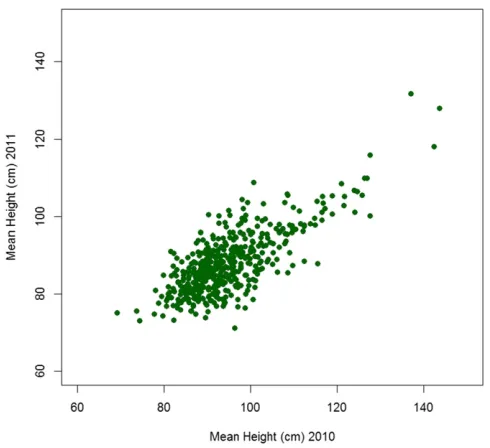
Height phenotypic data in multi-environment trials
An association mapping population of two-row spring barley lines was grown in a randomized spatial row-column design in two consecutive
trials in years 2010 and 2011 (i.e., two environments), withfive replicate plants of each line. At full maturity, the height of each plant was measured. The raw mean heights for lines grown in both years, and for which we have marker information, are shown in Figure 1. The plant height was slightly elevated in 2010 as opposed to 2011; the mean height in 2010 was 94.8 cm, and in 2011 was 87.9 cm. The correlation between the means of the line heights across the years was high at 0.76. These data were subsequently used, as described below, to develop our new GS model, and to predict, based only on the complement of lines with molecular markers present in each training set, the GEBV for height of lines that were in each validation set.
Comparison of models for whole genome prediction
Initially, thepartitioned,standard, andphenotypicmodels werefitted (Table 4) using the full data set, enabling the form ofum(Table 1), the
term representing marker variation, andue, the term representing
non-additive or residual genetic variance, to be established for use in the cross-validation. All models included a random term for replicate block for both trials; an additional random term was also included in the analysis to account for spatial variation present between columns in 2011.
Log-likelihood ratio tests comparing standardandpartitioned
models with the same form ofum(e.g., SDIAGvs.PDIAG, SCS+DIAGvs.
PCS+DIAG, etc.) were significant (P , 0.001), suggesting thepartitioned
models are superior to thestandardmodels (Table 4). In addition, all the MET models had lower AIC than the single trial year models, suggesting that the MET models were superior (Table 4). For two trials, the factor analytic models (EFAM1, SFAM1, and PFAM1), and the
unstruc-tured models (EUS, SUS, and PUS), respectively, are identical, and
there-fore the US results are shown with the FAM1model in Table 4. Given that the factor analytic model has been shown previously to improve the predictive accuracy of the line empirical BLUPs, that factor analytic models are easier tofit than an unstructured model (Kellyet al.2007), and given that we are primarily interested in models thatfit a main marker term, the US model is not discussed further.
For the phenotypic, standard, andpartitioned MET models, the compound symmetry form (ECS, SCSand PCS) had the highest AIC,
suggesting that this model was not a good choice in comparison to the other forms. The CS+DIAG forms (ECS+DIAGand PCS+DIAG) had similar
AICs to the factor analytic models (EFAM1and PFAM1). However, the
factor analytic model of thestandardmodel (SFAM1) showed a lower
AIC than the CS+DIAG form (SCS+DIAG). Examining the REML
estimates of the variance components (Table 5), it is clear that the CS+DIAG model does not necessarilyfit as well as the FAM1model, as the covariance between years has been constrained to be equal to the 2011 trial variance. However, as the variance component estimates of the CS+DIAG form (ECS+DIAG, SCS+DIAG, and PCS+DIAG) and the
FAM1form (EFAM1, SFAM1, and PFAM1) were similar for this data n Table 2 Number of lines with marker information in the groups used in the cross-validation
Groups for Cross-Validation
Number of Linesain Each Group
Total Number of Lines in Each Group (Total Number of Lines Across Groups) Commonb 2010 Only 2011 Only 2010 2011 METc
1–6 46 0 2 46 (276) 48 (288) 48 (288)
7–9 46 0 1 46 (138) 47 (141) 47 (141)
10 45 1 2 46 (46) 47 (47) 48 (48)
Total 459 1 17 460 476 477
a
These are the number of lines with marker information.
b
The common lines groups are kept the same across all analyses.
c
despite these constraints, both these forms were investigated further in the cross-validation. It is worth noting that Table 4 does not show the complete set of possiblepartitionedmodels. For thepartitioned
model, we have explored only models with the same form for theum
andueterms. It is, however, possible to include different forms for
each ofumandueterms, for example, the former could take a
com-pound symmetry form, and the latter a factor analytic form. When
fitting the FAM1model, the full parameterization requiredfive pa-rameters (one for the main effect, two loadings, and two specific variances), two more than the three required. Thus, when fitting the FAM1model, the two specific variances were constrained to be zero. Smithet al.(2001) discuss the parameter constraints necessary for FAkmodels withk . 1. Thus based on the results of the log-likelihood ratio tests, AIC, and estimates of the model variance com-ponents, for the MET analysis of trials in the cross-validation, we explore only the CS+DIAG and FAM1 forms for the marker and residual genetic effects. From the variance components of the diago-nal form of the phenotypic model, the heritability of the trials was calculated as 0.90 in 2010 and 0.75 in 2011, so both trials have high heritability. The difference in heritability between years reflects a greater contribution of environment to the variation in 2011, and consequently a lower proportion of variation that is genetic in that year. A comparison between the variance of theueterm from
pheno-typicand thepartitionedDIAG models (EDIAGand PDIAG,
respec-tively) enabled an estimate of the proportion of genetic variation accounted for by the markers, which was 0.75 for trial 2010, and 0.73 for trial 2011. The R code for determining the proportion of genetic variation is inFile S19.
The variance components of the residual terms in each year were higher in thestandardmodels compared to the equivalent forms of thephenotypic
andpartitionedmodels, particularly in 2011. The total genetic variation is therefore not accounted for in this model, perhaps as expected, given that the marker effect should reflect just additive genetic variation; the pro-portion of the genetic variation not being accounted for by the markers thus has contributed to the enlarged residual term. Given these limitations, thestandardmodels were not taken forward for cross-validation.
Cross-validation of selected models
The lines were randomly divided into 10 equivalent groups to facilitate comparative cross-validations, where the majority of lines were used as the training set, while 10%, 20%, or 40% of lines constituted the CV10, CV20, and CV40 validation sets, respectively (seeMaterials and Meth-odsand Table 3).
The cross-validation focuses on comparing thepartitionedand the
standardRR-BLUP model in each of three scenarios, which are each trial year separately (PDIAGand SDIAG, respectively), and in a joint MET
analysis of both years. From the initialfitting of the MET models just discussed, we examine only the models where the form ofumandue
takes either CS+DIAG (PCS+DIAGand SCS+DIAG, respectively), or FAM1
(PFAM1and SFAM1, respectively). Whenfitting thestandardand
partitioned models of the factor analytic form (SFAM1, PFAM1) in
ASReml, specific variances were set to zero as in the full data set, and the variance components of SFAM1were used as starting values
for the variance components of PFAM1.
Various comparisons between the predicted (GEBVs) and observed (GVs) results were made, and the performance of thepartitionedand
standardRR-BLUP models in terms of predictive ability of the markers was measured by the R-squared value (Table 6), while the accuracy of line estimates (GEBVs) was measured by the mean square error (Table 7). Both of these were averages across the iterations (Table 3).
In all three different CV evaluations [CV10, CV20, and CV40 (Table 3)], thepartitionedmodel showed a higher R-squared and lower MSE than the standardmodel, indicating that the predictive ability and accuracy of line estimates (GEBVs) were superior in thepartitioned
model. This supports thefinding of lower log-likelihoods and superior
fit of thepartitionedmodels as compared to thestandardmodels when the full data were used (Table 4). The R-squared decreased, and the MSE increased, as the number of lines in the training set decreases (going from CV10 to CV40) for the equivalent model (i.e., within the
partitioned models, or within the standard models), which was expected, as predictions were based on fewer lines. It should be noted that, except where the 2011 marker effects from the PDIAGmodel were
used to generate the GEBVs (Comparisons 2 and 3, Table 6), the R-squared in thepartitionedmodel in CV40 (where 40% of the lines were in the validation set) was similar to, or higher than, the R-squared of the standardmodel in CV10 (where 10% of the lines are in the validation set), suggesting the partitioned model was superior even when reducing the number of lines upon which the predictions are based. There was only a small compensating increase in MSE between thestandardmodel in CV10, and thepartitionedmodel in CV40, with the same exception of the 2011 marker effects from the PDIAGmodel
(Comparisons 2 and 3, Table 7), and also the main marker effects from the PFAM1, which showed larger increases (Comparison 12, Table 7).
These results shows that the partitioned model provides the best predictions of the height of lines in the validation set.
The results of the CV10 cross-validation were considered in more detail, bearing in mind that the other cross-validations (CV20 and CV40) reflect similar patterns. Initially, results where the equivalent of a single trial analyses was used to generate both GEBVs (PDIAGand SDIAG)
and GVs (EDIAG) were examined. Using the same trial year to generate
both the GEBVs and GVs (Comparisons 1 and 3, Table 6) gave the best results. The single trial analysis from 2010 showed a higher predictive ability than that from 2011 for thepartitionedmodel (0.461vs.0.334, Table 6), and for thestandardmodel (0.404vs.0.323, Table 6). This difference between the predictive ability in each year was initially sur-prising; given that there was a large overlap of individuals, the percent-age of variation explained by the markers was similar, and the observations were highly correlated across the 2 years. Thepartitioned
model showed a 5.7% and 1.1% improvement for 2010 and 2011, re-spectively, in predictive ability over thestandardmodel.
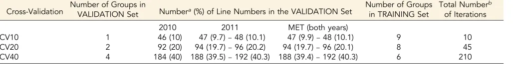
n Table 3 Summary of validation and training groups in three cross-validations
Cross-Validation Number of Groups inVALIDATION Set Numbera(%) of Line Numbers in the VALIDATION Set Number of Groups
in TRAINING Set
Total Numberb
of Iterations 2010 2011 MET (both years)
CV10 1 46 (10) 47 (9.7)–48 (10.1) 47 (9.9)–48 (10.1) 9 10 CV20 2 92 (20) 94 (19.7)–96 (20.2) 94 (19.7)–96 (20.1) 8 45 CV40 4 184 (40) 188 (39.5)–192 (40.3) 188 (39.4)–192 (40.3) 6 210
a
The number will be a range for 2011 and the MET as the number of lines in each group (Table 2) is variable.
b
If the opposite trial years were used to generate the GEBVs, then predicting 2010 GVs using the marker effects generated in 2011 (Comparisons 2, Table 6) had a higher predictive ability than the op-posite combination (Comparisons 4, Table 6), for both thepartitioned
andstandardmodels. Lyet al.(2013) suggested that G · E, which cannot be accounted for in a single trial, reduces the ability to make predictions. These results suggest that the 2011 heights had a higher environmental component than those observed in 2010, making pre-diction of the GEBVs from 2011 more difficult. We would therefore expect to be able to predict trial year 2011 better if a marker by trial interaction effect was included in a MET model, and this is exactly what was found, as discussed below.
The next comparisons are the MET analyses, where the GEBVs and GVs are based on a total effect found by summing the main or overall marker effect and the trial year marker effects. Thefirst thing to note is that for 2010 the CS+DIAG form forumhad around a 4–6% higher
predictive ability than the FAM1form in both thestandardand par-titionedmodels (Comparisons 5 and 7, Table 6). For 2011, the results were similar between the forms ofum(Comparisons 6 and 8, Table 6),
with around a 0.1% difference in predictive ability between the FAM1
form and the CS+DIAG form, with the latter showing only a slightly lower predictive ability, but a lower MSE. This suggests that the CS+DIAG form was superior to the FAM1form for this data set. Exploring different forms forumis clearly an important step in
determining the best model for GS.
The results for predictive ability were similar between the MET analysis and single year analysis for 2010 (Comparisons 5 and 1, 0.462 v 0.461,partitionedmodel, Table 6), but the MET shows a lower MSE (Comparisons 5 and 1, 7.35 v 7.47,partitionedmodel, Table 7). For 2011, the results of the MET were clearly superior over the single year analysis (Comparisons 6 and 3, Table 6), at 11.4% higher (0.448 v 0.334) for the partitioned model and 7.2% (0.395 v 0.323) for the
standardmodel. This suggests that using 2 years’data greatly improved the accuracy of the GEBVs by up to 11.4% for this data set. The benefit of including the marker by trial interaction effect was apparent in 2011 in particular, the year in which the results from the single trial analysis
suggested that the environment had a large influence on the results. The greater environmental influence in 2011 is consistent with the lower heritability and reduced genetic influence on plant height compared to the 2010 trial (see previous section). Greater environmental stress may also explain the lower mean height of lines in 2011.
Finally, we compared the GEBVS derived from the main marker effects in a MET analysis with the GVs derived from the single year analysis. Again the CS+DIAG form was superior to the FAM1form for
umin terms of predictive ability, and we therefore concentrated on the
former (Comparisons 9 and 10, Table 6). There was a reduction in predictive ability if the year specific marker effect was omitted when calculating the GEBVs, particularly for 2011 (0.448vs.0.336, Compar-ison 6 and 10, Table 6), where the environmental influence was higher. However, despite this reduction, a similar predictive ability to a single trial analysis was maintained, and the main effect still had a higher predictive ability than using the marker effects from the opposite year. For example, it is 3.5% higher in 2010 (Comparisons 9 and 2, 0.442vs.
0.407), and 1.7% higher in 2011 (Comparisons 10 and 3, 0.336 vs.
0.319), with correspondingly lower MSE.
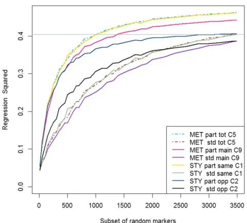
Implementing GS with a lower density of markers
A low density GS approach was considered, where, for each of the training sets of lines in CV10, the predictive ability of subsets of random markers was investigated. The results of the MET analyses and single trial analyses across the subsets of random markers were compared in each trial year (Figure 2 and Figure 3 for trial 2010 and trial 2011, respectively). Both plots showed that thepartitioned models have a much steeper incline within the subsets of random markers containing less than 500 markers than thestandardmodels, with the graphsfl at-tening out more than thestandardmodels as the marker numbers in subsets increase. This suggests that, for lower numbers of markers, the predictions were more accurate and reliable in thepartitionedmodel, and therefore fewer markers were required to obtain similar predic-tions. This would tend to support thefinding that the line estimates based on markers from the partitioned model were more accurate (lower MSE, Table 7) than those of thestandardmodel. The horizontal lines in Figure 2 and Figure 3 show the single trial year analysis of the
standardmodel using data from the same year. For trial 2010, all of the
partitioned models had superior predictive ability across the entire range of marker subsets (Figure 2), with the main improvements in predictive ability coming within the first 1000 or so markers. In the
standardRR-BLUP model, although there was an initial improvement in the predictive ability, this was less intense, and mostly small and steady over all of the latter marker subsets. This means that we can achieve the same predictive ability with the MET model as with the
standardRR-BLUP model using around 1000 markers, or around 2490 markers less than in the full higher-density GS. In 2011, thepartitioned
models had superior performance over thestandardsingle year model for lower numbers of markers, with thepartitionedMET model reach-ing the same level of prediction with only 500 markers.
DISCUSSION
In this paper, a method for genomic selection is proposed for the analysis of multi-environment crop trials. The method differs from other methods in a number of ways.
The method uses raw data observations at the plot, or pot, level rather than line means, thus incorporating line replication. This enables the total genetic variation due to lines to be partitioned into variation due to markers, and residual genetic variation, where the latter accounts for any genetic variation unexplained by the markers. The GEBVs, which are based on marker effects, are assumed mostly to reflect additive effects.
The residual genetic effect therefore should capture nonadditive effects. In inbred lines, the nonadditive effect will represent epistatic effects. However, in noninbred lines, other nonadditive effects will include dominance, inbreeding depression and homozygous dominance effects, the covariance between additive and dominance effects, and epistatic effects (de Boer and Hoeschele 1993).
Previous studies (Solberget al.2009; Crossaet al.2010; Burgueno
et al.2012) have included pedigree information, which captures a poly-genic effect as a way of accounting for nonadditive effects, and more recent studies (Daet al.2014; Munozet al.2014) have used marker-based relationships to separate additive and nonadditive variation. Da
et al.(2014) only included additive and dominance relationship matri-ces. Munozet al.(2014) included, in addition,first-order epistatic re-lationship matrices (additive by additive, dominance by dominance, and additive by dominance); however, their approach has the disad-vantage that the resulting genetic effects are nonorthogonal, and there is dependency between some of the estimates of the additive and non-additive variance components, as thefirst-order epistatic relationship matrices they form are based on Hadamard products of the additive and dominance relationship matrices. This means that the matrices may not be capturing all nonadditive variation. Also, given the number of relationship matrices necessary to account for nonadditive variation, extension to a MET model may be difficult. In contrast, the residual genetic effect representing nonadditive effects found in our model is more encompassing and less restrictive, and should capture all non-additive effects. It is, however, worth noting that, because of thefl ex-ibility of the linear mixed model, additional relationships matrices may also be added to our model if required. For example, if pedigree information was available, a single polygenic effect could be added, or it may be possible to further partition our residual genetic effects by the addition of further genomic relationship matrices, for instance, a ge-nomic dominance matrix could be added in the case of hybrid crops.
Recent studies have shown that maximum prediction was reached when the breeding value was based on both additive and nonadditive effects (Daet al.2014; Munozet al.2014), and Lyet al.(2013) notes that considering only the additive component may underestimate predic-tion accuracy. Here, we have only investigated the use of the additive
proportion of the total genetic effect as described by the markers for the prediction of breeding values where, for future lines,onlymarker in-formation is available. We found that partitioning the total genetic variation into marker and residual genetic variation, and using the improved predictive ability of the marker additive genetic effects for future predictions, gave more accurate estimates even for the single trial analysis than was the case if the total genetic variation was not parti-tioned (i.e., whenfitting thestandardmodel, which excluded the re-sidual genetic and therefore nonadditive, variation). Improvements of up to 5.7% in predictive ability were found. Further work is required to determine whether improved prediction can be achieved by using the total genetic effect (as opposed to the total genetic effect from markers) of a line from thepartitionedmodel for phenotypic evaluation. The value of using the total genetic effect (additive plus nonadditive) for phenotypic evaluation would depend on the impact of the nonadditive proportion. If the nonadditive proportion of variation was reasonably high, the use of the total genetic effect for phenotypic evaluation would be important. However, it is worth noting the total genetic effect does not reflect the potential of a line as a parent as nonadditive effects are not inherited, although it may better predict the commercial viability of a line and may be useful in determining which lines to take forward from a breeding program for elite development.
Using the raw data in a single stage approach has the added advantage that it allows spatial variation to be incorporated into the analysis, enabling joint estimation of all effects, genetic and nongenetic. This is the preferred option, as the precorrection of data necessary in a two stage approach can have undesirable consequences, such as biased estimates of marker effects, and induced correlations between residuals (de los Camposet al.2013).
It was evident from the analysis that thestandardmodel had an inflated trial residual (error) term compared to thepartitionedmodel. Thepartitionedmodel enabled the additive variation due to markers to be estimated, and it was found to account for approximately 75% of the total genetic variation in each of the trials. In thestandardmodel, the inflation of the trial residual term, while apparent, was not sufficient to explain all of the unaccounted nonadditive genetic variation. This suggests that, in thestandardmodel, some of the omitted nonadditive
n Table 4 Summary of the modelsfitted to the full data set
Modela Formbofu
m Form ofue STY or MET Log-Likelihood AIC
Phenotypicc E
DIAG DIAGd STY 211,074.6 22,163.1
ECS CSe MET 210,877.0 21,768.1
ECS+DIAG CS+DIAGf MET 210,872.5 21,760.9
EFAM1, EUS FAM1g, USh MET 210,872.4 21,760.8
Standardi S
DIAG DIAG STY 210,924.9 21,863.8
SCS CS MET 210,794.0 21,602.1
SCS+DIAG CS+DIAG MET 210,790.6 21,597.2
SFAM1, SUS FAM1, US MET 210,787.8 21,591.6
Partitionedj P
DIAG DIAG DIAG STY 210,876.4 21,770.8
PCS CS CS MET 210,747.2 21,512.5
PCS+DIAG CS+DIAG CS+DIAG MET 210,744.6 21,511.2
PFAM1, PUS FAM1, US FAM1, US MET 210,744.2 21,510.4 STY, single trial year; MET, multi-environment trial; AIC, Akaike information criteria.
a
All models derive from Equation 1 but are special cases ofg (Equation 2).
b
Details of forms ofumare given in Table 1.
c
Phenotypic model hasg=ue.
d
DIAG implies the covariance between the two trials is assumed to be zero, and is equivalent tofitting the two trials separately.
e
CS is the compound symmetry model.
f
CS+DIAG is the model described by Culliset al.1998.
g
FAM1is the factor analytic model (Smithet al.2001), with main effect withkthe number of factors equal to 1.
h
US is the unstructured model (US), for two trials this model is equivalent to the FAM1model.
i
Standard RR-BLUP model hasg¼ ðIs5MÞum.
j
genetic variation is incorporated into the estimate of the genetic var-iation due to the markers, and they do not therefore reflect purely additive variation. This perhaps explains why, in thestandardmodel, the marker effects are not as good for prediction of GEBVs, and this model showed higher MSE of prediction. The outcome is that esti-mates of marker effects from thepartitionedmodel should be less biased, be more likely to reflect additive variation, and therefore lead to better estimation for future prediction.
The single trial RR-BLUPpartitionedmodel was extended to enable a multi-environment approach to analysis. Analyzing trials under the
partitionedRR-BLUP model in a MET setting extends a phenotypic MET model in an intuitive manner. In the GS model, we implicitly included both a main effect for markers, and a marker by trial inter-action term. We found that a main marker effect in an analysis of trials in a MET was a useful predictor, even when a strong marker by trial interaction was present. These main marker effects seem to reflect a more ‘stable’proportion of the marker, and were shown to have a predictive ability slightly superior to a single trial analysis. Presumably, the addition of more trials would improve the robustness of the main marker effect to G · E.
The RR-MET (partitionedandstandard) performed well particu-larly where there was a larger environmental influence. In the example data set, in the 2011 trial, improvements of the MET over the single trial analysis of as much as 11.4% were seen, probably due to the inability of a single year analysis to account for the marker by trial variation. The poorer performance found when using 2011 marker effects to predict 2010 supports the observation of Lyet al.(2013) that the presence of G · E reduces the ability to make predictions in locations where no evaluations have previously been done. MET analysis uses the correla-tion between trials to improve prediccorrela-tion of lines (Smithet al.2005). Where the environmental influence was lower, as in the 2010 trial, the
partitionedsingle trial model performed well, with similar predictive ability to thepartitionedMET model, but with lower MSE in the latter. As in Guoet al.(2013), gains here are attributable to the more accurate estimates of trial-specific marker effects through utilizing genetic cor-relations. In our cross-validation approach, we excluded validation lines from both trials, and found that, in 2011, where environmental influence was large, the MET was superior to the single trial analysis. Burguenoet al.(2012) and Guoet al.(2013) also looked at MET verses single trial analysis and included cross-validation schemes (referred to as CV1 in both papers), which also excluded validation lines from all environments. Our findings are contrary to those of Burguenoet al.
(2012), who found no improvement in predictability of a MET over a single trial analysis, but support thefindings of Guoet al.(2013), who found similar average gains in prediction accuracies of up to 10%.
In terms of using a subset of the markers in a low density GS approach, similar predictive ability could be gained with a much lower number of markers in thepartitionedMET model, particularly in 2011. The results suggest that thepartitionedmodel increased the accuracy of the marker effects with further gains to be had by using the MET model, particularly if the environmental influence on results is high (as in 2011). When examining the value of predictive ability of random sub-sets of markers, some subsub-sets were superior to others (results not shown). Examining markers that are consistently found in the highly predictive subsets may lead to suitable choices for a MARS approach, and this may be worth exploring when considering the practical and optimal use of markers in GS in crops. Finally, as Heffneret al.(2011a, 2011b) have found, reducing the number of lines in a training popu-lation decreases the predictive ability. However, our observations sug-gest that thepartitionedmodel goes some way to alleviating this effect.
In summary, thepartitionedMET model used here is a single linear mixed model that incorporates trial, residual genetic-by-trial interac-tions, and trial-specificfield and randomization-based terms, in a ran-dom RR-BLUP setting for marker effects and their interaction with trials. The MET model offers a viable,flexible addition to the GS tool box.
ACKNOWLEDGMENTS
The authors thank everybody who helped with the planting, harvest-ing, and samplharvest-ing, particularly Reza Shafiei, who supervised much of the phenotyping, and Nicola Uzrek, who played a major role in coordinating plant and seed maintenance and health. Thanks to the Biotechnology and Biological Sciences Research Council (BBSRC), whofinancially supported this work through the BBSRC Sustainable Bioenergy Centre (BSBEC) grant number BBG0162321, and to the Scottish Government Centre of Excellence in Climate Change (CXC, 2011–2016). C.H. is a Royal Society Wolfson Research Merit Award holder.
Author contributions: H.O. designed the field phase in 2011, developed the statistical models and conducted the statistical analysis, interpreted the statistical data, and drafted the manu-script. B.C. and R.T. developed the statistical models, and assisted with the statistical analysis. J.C. designed thefield phase in 2010, assembled the plant material, and coordinated sowing and growing of both the 2010 and 2011 trials. R.W. provided the marker data used for genetic analysis. C.H. and R.W. jointly conceived and won the research funding to conduct the work, and oversaw design and
implementation of both seasons’experimental data collection; both contributed to writing the manuscript. All authors read and ap-proved thefinal manuscript.
LITERATURE CITED
Akaike, H., 1974 New look at statistical-model identification. IEEE Trans-actions on Automatic Control. AC19: 716–723.
Burgueno, J., G. de los Campos, K. Weigel, and J. Crossa, 2012 Genomic prediction of breeding values when modeling genotype·environment interaction using pedigree and dense molecular markers. Crop Sci. 52: 707–719.
Butler, D., B. Cullis, A. Gilmour, and B. Gogel (Editors), 2009 ASReml R-reference manual, VSN International Ltd., Hemel Hempstead, UK. Comadran, J., B. Kilian, and J. Russell, L. Ramsay, N. Steinet al.,
2012 Natural variation in a homolog ofAntirrhinum CENTRORA-DIALIS contributed to spring growth habit and environmental adapta-tion in cultivated barley. Nat. Genet. 44: 1388–1392.
Crossa, J., G. de los Campos, P. Perez, D. Gianola, J. Burguenoet al., 2010 Prediction of genetic values of quantitative traits in plant breeding using pedigree and molecular markers. Genetics 186: 713–724. Crossa, J., P. Perez, G. de los Campos, G. Mahuku, S. Dreisigackeret al.,
2011 Genomic selection and prediction in plant breeding. J. Crop Im-prov. 25: 239–261.
Cullis, B., B. Gogel, A. Verbyla, and R. Thompson, 1998 Spatial analysis of multi-environment early generation trials. Biometrics 54: 1–18. Cullis, B., A. Smith, and N. Coombes, 2006 On the design of early generation
variety trials with correlated data. J. Agric. Biol. Environ. Stat. 11: 381–393. Da, Y., C. Wang, S. Wang, and G. Hu, 2014 Mixed model methods for
genomic prediction and variance component estimation of additive and dominance effects using SNP markers. PLoS One 9: e87666.
Figure 3 Comparison ofpartitionedversesstandardRR-BLUP model of CV10 (Table 3) for different forms (Table 1) and comparisons (Table 6), for trial year 2011 across a range of subsets of random markers. The horizontal line is maximum predictive ability of thestandardsingle trial year analysis for 2011. Each subset represents the average results from 200 different sets of random markers, the comparisons across analyses are on the same subsets of random markers. MET, multi-environment trial analysis; STY, single trial year analysis; part,partitionedmodel; std, standardmodel; total, main marker effect + marker by trial in-teraction effect; main, main marker effect; same, same year used for prediction (2011 GEBV used to predict 2011 GV); opp, opposite year used for prediction (2010 GEBV used to predict 2011 GV); C, see Comparison as per Table 6 for more detail.
de Boer, I. J. M., and I. Hoeschele, 1993 Genetic evaluation methods for pop-ulations with dominance and inbreeding. Theor. Appl. Genet. 86: 245–258. de los Campos, G., J. Hickey, R. Pong-Wong, H. Daetwyler, and M. Calus,
2013 Whole-genome regression and prediction methods applied to plant and animal breeding. Genetics 193: 327–345.
Desta, Z. A., and R. Ortiz, 2014 Genomic selection: genome-wide predic-tion in plant improvement. Trends Plant Sci. 19: 592–601.
Gilmour, A., B. Cullis, and A. Verbyla, 1997 Accounting for natural and extraneous variation in the analysis offield experiments. J. Agric. Biol. Environ. Stat. 2: 269–293.
Guo, Z., D. M. Tucker, D. Wang, C. J. Basten, E. Ersozet al., 2013 Accuracy of across-environment genome wide prediction in maize nested associa-tion mapping populaassocia-tions. G3 (Bethesda) 3: 263–272.
Habier, D., R. Fernado, and J. Dekker, 2007 The impact of genetic rela-tionship information on genome assisted breeding values. Genetics 177: 2389–2397.
Habier, D., R. Fernando, and D. Garrick, 2013 Genomic BLUP decoded: a look into the black box of genomic prediction. Genetics 194: 597–607. Hastie, T., R. Tibshirani, B. Narasimhan, and G. Chu, 2014 impute: Im-putation for microarray data. R package version 1.36.0. Available at: https://bioconductor.org/packages/release/bioc/html/impute.html. Accessed: April 21, 2014.
Heffner, E. L., A. J. Lorenz, J.-L. Jannink, and M. E. Sorrells, 2010 Plant breeding with genomic selection: gain per unit time and cost. Crop Sci. 50: 1681–1690.
Heffner, E. L., J.-L. Jannink, H. Iwata, E. Souza, and M. E. Sorrells, 2011a Genomic selection accuracy for grain quality traits in biparental wheat populations. Crop Sci. 51: 2597–2606.
Heffner, E. L., J.-L. Jannink, and M. E. Sorrells, 2011b Genomic selection accuracy using multifamily prediction models in a wheat breeding pro-gram. Plant Genome 4: 65–75.
Heslot, N., H.-P. Yang, M. Sorrells, and J.-L. Jannink, 2012 Genomic se-lection in plant breeding: a comparison of models. Crop Sci. 52: 146–160. Jannink, J., A. Lorenz, and H. Iwata, 2010 Genomic selection in plant
breeding: from theory to practice. Brief. Funct. Genomics 9: 166–177. Jonas, E., and D.-J. De Koning, 2013 Does genomic selection have a future
in plant breeding? Trends Biotechnol. 31: 497–504.
Kelly, A. M., A. B. Smith, J. A. Eccleston, and B. R. Cullis, 2007 The accuracy of varietal selection using factor analytic models for multi-en-vironment plant breeding trials. Crop Sci. 47: 1063–1070.
Lado, B., I. Matus, A. Rodriguez, L. Inostroza, J. Polandet al.,
2013 Increased genomic prediction accuracy in wheat breeding through spatial adjustment offield trial data. G3 (Bethesda) 2: 2015–2113. Ly, D., M. Hamblin, I. Rabbi, G. Melaku, M. Bakareet al., 2013 Relatedness
and genotype·environment interaction affect prediction accuracies in genomic selection: a study in cassava. Crop Sci. 53: 1312.
Massman, J. M., H.-J. G. Jung, and R. Bernardo, 2013 Genomewide selec-tion verses marker-assisted recurrent selecselec-tion to improve grain yield and stover-quality traits for cellulosic ethanol in maize. Crop Sci. 53: 58–66.
Meuwissen, T. H. E., B. J. Hayes, and M. E. Goddard, 2001 Prediction of total genetic value using genome-wide dense marker maps. Genetics 157: 1819–1829.
Munoz, P. R., M. F. R. J. Resende, S. A. Gexan, M. D. V. Resende, G. de los Camposet al., 2014 Unravelling additive from nonadditive effects using genomic relationship matrices. Genetics 198: 1759–1768.
Oakey, H., R. Shafiei, J. Comadran, N. Uzrek, B. Culliset al.,
2013 Identification of crop cultivars with consistently high lignocellu-losic sugar release requires the use of appropriate statistical design and modelling. Biotechnol. Biofuels 6: 185.
Patterson, H. D., V. Silvey, M. Talbot, and S. T. C. Weatherup,
1977 Variability of yields of cereal varieties in U. K. trials. J. Agric. Sci. 89: 238–245.
Piepho, H., J. Ogutu, T. Schulz-Streeck, B. Estaghvirou, A. Gordilloet al., 2012 Efficient computation of ridge-regression best linear unbiased prediction in genomic selection in plant breeding. Crop Sci. 52: 1093– 1104.
R Core Team, 2015 R: A language and environment for statistical com-puting. R Foundation for Statistical Computing, Vienna, Austria. Avail-able at:http://www.R-project.org/.
Smith, A., B. Cullis, and R. Thompson, 2001 Analyzing variety by envi-ronment data using multiplicative mixed models and adjustments for spatialfield trend. Biometrics 57: 1138–1147.
Smith, A., B. Cullis, and R. Thompson, 2005 The analysis of crop cultivar breeding and evaluations trials: an overview of current mixed model approaches. J. Agric. Sci. 143: 1–14.
Solberg, T. R., A. K. Sonesson, J. a. Wooliams, J. Ødegard, and T. H. E. Meuwissen, 2009 Persistence of accuracy of genome-wide breeding values over generations when including a polygenic effect. Genet. Sel. Evol. 41: 53.
Stranden, I., and D. Garrick, 2009 Technical note: derivation of equivalent computing algorithms for genomic predictions and reliabilities of animal merit. J. Dairy Sci. 92: 2971–2975.
Tibshirani, R., 1996 Regression shrinkage and selection via the LASSO. J. R. Stat. Soc., B 58: 267–288.
Wang, C.-L., P.-P. Ma, Z. Zhang, X.-D. Ding, J.-F. Luiet al.,
2012 Comparison offive methods for genomic breeding value estima-tion for the common dataser of the 15th QTL-MAS workshop. BMC Proc. 6(Suppl 2): S13.
Wimmer, V., C. Lehermeier, T. Albrecht, H.-J. Auinger, Y. Wanget al., 2013 Genome-wide prediction of traits with different genetic architec-ture through efficient variable selection. Genetics 195: 573–587. Zhong, S., J. Dekker, R. Fernado, and J.-L. Jannink, 2009 Factors affecting
accuracy from genomic selection in populations derived from multiple inbred lines: a Barley case study. Genetics 182: 355–364.
Zou, H., and T. Hastie, 2005 Regularization and variable selection via the elastic net. J. R. Stat. Soc. Ser. A Stat. Soc. 67: 301–320.