Practice and philosophy of climate model tuning across six US modeling centers

https://doi.org/10.5194/gmd-10-3207-2017 © Author(s) 2017. This work is distributed under the Creative Commons Attribution 3.0 License.

Practice and philosophy of climate model tuning across six US

modeling centers

Gavin A. Schmidt1, David Bader2, Leo J. Donner3, Gregory S. Elsaesser1,4, Jean-Christophe Golaz2, Cecile Hannay5, Andrea Molod6, Richard B. Neale5, and Suranjana Saha7

1_{NASA Goddard Institute for Space Studies, 2880 Broadway, New York, USA} 2_{DOE Lawrence Livermore National Laboratory, Livermore, California, USA}

3_{GFDL/NOAA, Princeton University Forrestal Campus, 201 Forrestal Rd., Princeton, New Jersey, USA} 4_{Columbia University, New York, New York, USA}

5_{National Center for Atmospheric Research (NCAR), Boulder, Colorado, USA} 6_{Global Modeling and Assimilation Office, NASA GSFC, Greenbelt, Maryland, USA}

7_{Environmental Modeling Center, NCEP/NWS/NOAA, NCWCP College Park, Maryland, USA}

Correspondence to:Gavin A. Schmidt ([email protected]) Received: 2 February 2017 – Discussion started: 14 February 2017

Revised: 17 July 2017 – Accepted: 24 July 2017 – Published: 1 September 2017

Abstract.Model calibration (or “tuning”) is a necessary part of developing and testing coupled ocean–atmosphere climate models regardless of their main scientific purpose. There is an increasing recognition that this process needs to become more transparent for both users of climate model output and other developers. Knowing how and why climate models are tuned and which targets are used is essential to avoiding pos-sible misattributions of skillful predictions to data accommo-dation and vice versa. This paper describes the approach and practice of model tuning for the six major US climate mod-eling centers. While details differ among groups in terms of scientific missions, tuning targets, and tunable parameters, there is a core commonality of approaches. However, prac-tices differ significantly on some key aspects, in particular, in the use of initialized forecast analyses as a tool, the ex-plicit use of the historical transient record, and the use of the present-day radiative imbalance vs. the implied balance in the preindustrial era as a target.

1 Introduction

Simulation has become an essential tool for understanding processes in the Earth system, interpreting observations and for making predictions over short (weather), medium (sea-sonal), and long (climate) terms. The complexity of this

sys-tem is evident in the myriad processes involved (such as the microphysics of cloud nucleation, land surface heterogene-ity, convective plumes, and ocean mesoscale eddies) and in the dynamic views provided by remote sensing. This com-plexity and wide range of scales that need to be incorporated imply that simulations will necessarily include approxima-tions to well-understood physics and empirical formulaapproxima-tions for unresolved effects. The simulations are neither a straight-forward encapsulation of some well-known theory, nor are they laboratory experiments probing the real world, though they have features of both (Schmidt and Sherwood, 2014). Despite this, climate and weather simulations have demon-strated useful predictive skill across many emergent diagnos-tics (Reichler and Kim, 2008; Flato et al., 2013; Bosilovich, 2013). Note that we distinguish fields or statistics in the model that arise from the interactions of multiple physical effects (“emergent properties”) from those that are closely related to single processes or parameterizations.

com-plexity has grown, more processes are explicitly included and the parameterizations are pushed to a more detailed (and more fundamental) level, allowing for better constraints on unknown parameters. However, at the same time, the process of model development has become more convoluted and now involves many more components than it did originally. This has led somewhat predictably to an unfortunate reduction in transparency over time.

It is worth expanding on why this matters: first, model de-velopment involves expert judgments which are inevitably subjective, and with different choices there would be dif-ferences in emergent responses. For instance, in the MPI model, Mauritsen et al. (2012) show that equally valid but distinct tunings can impact model sensitivity. This kind of be-havior should therefore be reported more widely to improve the assessment of the robustness of specific responses. Sec-ond, models used as part of international assessment projects (such as the Coupled Model Intercomparison Project, Phase 5: CMIP5) are increasingly being weighted or subset in order to refine predictions. If the skill measure that is used to fil-ter or weight models has been tuned for in some cases rather than in others, the subset or weighted average will be biased towards models where the skill measure was tuned over those in which it was not, and that may not correspond to better physics or better predictions (Knutti et al., 2010).

Thus it has become increasingly clear that a more trans-parent process is necessary. A survey of modeling groups in-volved in CMIP5 (Hourdin et al., 2017, hereafter H17) pro-vides a good background on tuning practices and makes a plea for better coordination of documentation of these issues. This paper is a more detailed follow-up for a subset of cli-mate models associated with laboratories in the US (three of which were surveyed by H17, three of which were not). The six modeling centers that are the focus of this paper have all developed and maintained Earth system models that (at minimum) have a dynamic atmosphere and coupled ocean components and are global in scope. Additional components (such as ice sheets, the carbon cycle, atmospheric chemistry, and aerosols) are also common. While two of the models dis-cussed (NCEP Climate Forecast System (CFS) and GEOS-5 (Goddard Earth Observing System 5) from NASA GMAO) are primarily used for short-term (daily to seasonal) predic-tions, there is sufficient overlap with the models focused on longer-term problems (decadal to multidecadal periods) to warrant describing them all as “climate models” below.

2 Why is climate model tuning necessary?

Climate and weather models consist of three levels of rep-resentation of physical processes: fundamental physics (such as conservation of energy, mass and momentum), approxi-mations to well-known physical theories (the discretization of the Navier–Stokes equations, broadband approximations to line-by-line radiative transfer codes, etc.), and empirical

approximations (“parameterizations”) needed to match the phenomenology of unresolved or poorly understood subgrid-scale or excluded processes (Hourdin et al., 2017). The de-gree of approximation and complexity in the empirical pa-rameterizations vary greatly across models and processes, as well as the resolved scales. Many parameterizations em-ploy an underlying paradigm that makes use of well-known or well-observed processes so that the fundamental depen-dence on the atmospheric state is approximated, albeit only at a phenomenological level.

Parameters in climate models vary widely in their phys-ical interpretation. Some are well-determined physphys-ical val-ues, such as the Coriolis parameter, the acceleration due to gravity, or the Stefan–Boltzmann constant. Some, such as reaction rates for chemical or microphysical processes, may be inferred from laboratory or field measurements (with some uncertainty). Some emerge from the construction of parameterizations but do not correspond directly to well-defined physical processes, e.g., “erosion rates” for clouds (Tiedtke, 1993). Others also emerge from the characteriza-tion of model subgrid-scale variacharacteriza-tions in the parameteriza-tions, such as the “critical relative humidity” for cloud forma-tion (Schmidt et al., 2006), or equivalent mixing rates for tur-bulent transport, and may be loosely approximated from ei-ther observations or higher-resolution models (e.g., Siebesma and Cuijpers, 1995).

Individual parameterizations for a specific phenomenon are generally calibrated to process-level data using high-resolution modeling and/or field campaigns to provide con-straints. For instance, boundary layer parameterizations might be tuned to well-observed case studies such as in Larcfrom (Pithan et al., 2016) or DICE (http://appconv. metoffice.com/dice/dice.html). However, in some cases, even when parameter values are well constrained physically or ex-perimentally, simulations can often be improved by choos-ing values that violate these constraints. For example, Go-laz et al. (2011) found that cooling by interactions between anthropogenic aerosols and clouds in GFDL’s AM3 model depends strongly on the volume-mean radius at which cloud droplets begin to precipitate. By altering CM3 after its con-figuration used for CMIP5 was established as described in Donner et al. (2011), Golaz et al. (2013) found that its 20th-century temperature increase could be simulated more real-istically (larger increase) using values for this threshold drop size smaller than observed (Pawlowska and Brenguier, 2003; Suzuki et al., 2013) (see Sect. 4.1 below). Another example is the variation in the effective diffusion constants for mo-mentum, moisture, and temperature, which has been used to decrease large root-mean-square errors in tropical winds in the NCEP model.

model against a selected set of target observations. The deci-sions on what to tune, and especially what targets to tune for, undoubtedly involve value judgments (Hourdin et al., 2017; Winsberg, 2012; Schmidt and Sherwood, 2014; Inte-mann, 2015). Notably, there is not any obvious consensus in the modeling community as to the extent to which parame-ter choices should be guided by conforming to process-level knowledge as opposed to optimizing emergent behaviors in climate models. At many centers, the philosophy for the most part has been to tune parameters in ways that make physical sense, with the expectation that in the long run that should be the best strategy. Increasing skill in climate models over time does support this approach (Reichler and Kim, 2008).

Additionally, climate simulations depend not only on pa-rameter choices within an established model structure but also on the structural choices made in the parameteriza-tion itself. Examples include experimentaparameteriza-tion with alternate closures and triggers for the cumulus parameterization at GFDL during the development of GFDL AM3 (Benedict et al., 2013) and evaluation of two candidate parameteri-zations for cloud macrophysics and convection in NCAR CESM2 (Community Earth System model 2) (Bogenschutz et al., 2013; Park, 2014). Theoretically, all such structural choices could be coded to vary with a parameter and so there is no strong theoretical distinction between parameter and structural variations. In practice, however, perturbed physics ensembles (PPEs) do not span as wide a range of structural variations as multimodel ensembles of opportunity (Yoko-hata et al., 2012). These examples suggest that it can be hard to distinguish model tuning from model development (writ large) in practice, since both happen concurrently. For our purposes, we define tuning as a change occurring within a fixed structural framework that does not involve adding new physics.

Targets for possible tuning fall into three classes. First there are targets that need to be satisfied in order for use-ful numerical experiments to be performed in the first place (usually related to the equilibration of model components with long timescales). The most important of these is a re-quirement of near energy balance at the top of the atmo-sphere and surface in an initial state of a coupled model to prevent temperature drifts over time. Strictly speaking this is not tuning to an observed quantity, but rather is a tuning to a situation that was approximately inferred to hold in the “preindustrial” (PI) period. Note that while the concept of a preindustrial period is a little elusive (Hawkins et al., 2017), we refer to conditions around the mid-19th century around 1850. To avoid dealing with the lack of sufficient observa-tional data from the 19th century, some modeling groups (see below) alternatively choose to tune to present-day (PD) conditions, including an energy imbalance at the top of the atmosphere (TOA) as inferred from ocean observations to-day (Loeb et al., 2009). Another tuning target is sometimes referred to as the radiative forcing perturbation (RFP), or the effective radiative forcing, and is the change in net flux

which occurs in a multiyear integration with specified cli-matological sea surface temperatures (SSTs) when emissions (primary aerosols and short-lived gases), long-lived green-house gas (GHG) concentrations (carbon dioxide, nitrous ox-ide, methane, and the halocarbons), and solar irradiance are changed from preindustrial to present-day values.

A second class of tuning targets are well-characterized cli-matological observations which might include annual means, average seasonal cycles, or interannual variance. A third po-tential class are observations of transient events (on daily to centennial scales) or trends. Some observational targets have important (and sometimes unrecognized) structural uncer-tainties and therefore any tuning to those targets risks over-fitting the model to imperfect data, potentially reducing skill in “out-of-sample” predictions (those for which the evalu-ation data either did not exist at the time of the prediction or were not used in model development or tuning). This is a particular problem for transient observations such as esti-mates of early 20th-century temperature changes (Thompson et al., 2008; Richardson et al., 2016), pre-1979 sea-ice extent (Meier et al., 2012; Walsh et al., 2017), pre-1990 ocean heat content change (Levitus et al., 2000; Church et al., 2011), or water vapor trends (Dessler and Davis, 2010), which have all been corrected in recent years, as nonclimate artifacts in the raw observations have been found and adjusted for. In con-trast, many climatologies over the satellite era are robust met-rics whose estimates over any fixed period have not changed appreciably as understanding of the observations evolved.

Models equipped for data assimilation or that are used for operational forecasts have the additional possibility of tuning parameters to improve skill scores in those forecasts on mul-tiple timescales – whether they be 6-hourly, daily, weekly, or even for many months for seasonal forecasts of, for instance, the state of the tropical Pacific.

We note here a distinction between fields that are closely monitored during the model development process (many ex-amples are given below) and specific tuning targets. Moni-tored diagnostics tend to be complex emergent diagnostics that do not depend in any simple way on adjustable param-eters, and thus are difficult (or impractical) to tune for. For example, note that the range of preindustrial global tem-peratures in CMIP5 is [12.0,14.8]◦C, which is noticeably wider than the uncertainties in that quantity (±0.5◦C; Jones et al., 2012). Changes in such a monitored field are kept track of, but unless the values stray beyond a nominal acceptable range no action to change the code would be taken. If the values do stray, the principal action is often taken to go into detail and examine what has happened more closely.

one field are often accompanied by degradation in others, and thus the final choice of parameters involves subjective judg-ments about the relative importance of different aspects of the simulations. For example, the Australian contribution to CMIP5 (ACCESS v.1) used a version of the UK Met Office atmosphere model with small modifications to mitigate prob-lems in the tropics and Southern Hemisphere that affect Aus-tralian forecasts, at the expense of performance elsewhere (Bi et al., 2013). There are additionally many obvious biases in model simulations that persist across model generations, in-dicating that these aspects are robustly stubborn to develop-ment changes in the model (including the tuning) (Masson and Knutti, 2011).

Most discussions of tuning deal with explicit calibration of parameters to match a target observation. However, analy-sis of the CMIP3 ensemble (Kiehl, 2007; Knutti, 2008) sug-gested that there may have been some kind of implicit tun-ing related to aerosol forctun-ing and climate sensitivity among a subset of models, with models with higher sensitivity hav-ing a tendency to have higher (more negative) aerosol forc-ing (this situation was less evident in CMIP5; Forster et al., 2013). Both of these correlations, however, seem rather low (CMIP3: 0.24; CMIP5: 0.19) and so do not provide evidence for a general tuning related to forcing and sensitivity. That models with accurate historical simulations must trade off forcing and sensitivity is not necessarily evidence they have been tuned to do so. Since the CMIP3 models’ aerosol forc-ings were not explicitly tuned to enforce the observed his-torical trend in temperature, the mechanisms that might ex-plain this observation are unclear. With further data on the current top-of-atmosphere radiative imbalance (Allan et al., 2014; von Schuckmann et al., 2016), this issue will, however, need to be revisited for the latest generation of models.

Model selection can also act as an implicit form of tun-ing, even though this might be seen by others as simple model development. In deciding between two versions of a dynamical core or convection parameterizations, skill in El Niño–Southern Oscillation (ENSO) variability or reductions of ocean drifts may play an important role. Conceivably, a modeling center may decide not to release or use a particular version because it fails to meet certain criteria perceived to be essential, though more generally this will simply spur further development. One candidate criterium would be a realistic simulation of the 20th century; however, the wide spread in 20th-century trends in the CMIP5 ensemble (Forster et al., 2013, Fig. 7) would indicate that this has not been generally applied (though see below for more detailed discussion of the use of historical changes).

Within climate models, there is always a choice as to whether to tune a specific component (such as the atmo-sphere, sea ice, land surface, or ocean) with tightly con-strained boundary conditions or to tune the coupled model as a whole. In practice, both approaches are taken, though the relative importance and computation resources available vary across groups. Tuning components is generally fast and

efficient, but does not necessarily prove robust when those components are coupled. However, coupled models take a very long time to equilibrate, and their quasi-stable states may be too far from the observed climate to be useful. As-suming that models conserve energy appropriately, all con-trol runs will eventually drift to a quasi-steady state with a near-zero energy balance at the TOA and at the surface of the ocean. However, the realism of the final state is not guaran-teed and, indeed, given the long time constants in the ocean, might require many thousands of years of integration to get to the wrong answer. Thus a balance must be struck between approaches.

3 Specific practices

Each of six US modeling centers described below have spe-cific missions and foci that drive different aspects of their modeling. For instance, NASA GMAO and NCEP have op-erational data assimilation products for short-term weather, longer seasonal forecasts, and reanalyses that form the core of their tasks. NCAR CESM, GFDL, and NASA GISS have more long-term climate change issues at the forefront of their research, but each with different mandates – respectively, to be a community model, to advance NOAA’s mission goal to understand and predict changes in climate, and to help in-terpret and use NASA remote sensing products. The DOE’s Accelerated Climate Modeling for Energy (ACME) project has been tasked with a very specific role to serve DOE’s en-ergy planning and computational resource needs.

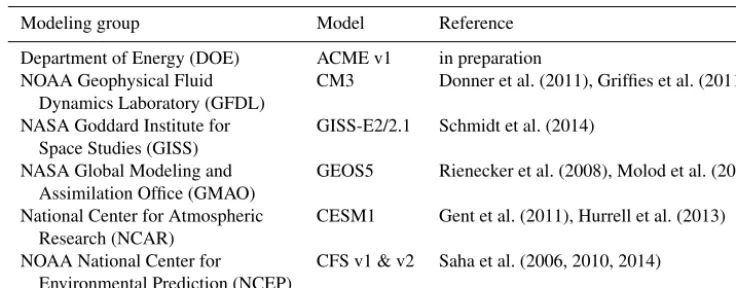
For each modeling group, we describe the principal tar-gets and tuning strategies for their atmosphere-only GCM (general circulation model), their coupled ocean–atmosphere GCM, and additional Earth system components as relevant. The specific models referred to are described in Table 1. We outline the commonalities of approaches and key differences in Sect. 4, and then discuss the implications and ways for-ward in Sect. 5.

3.1 DOE

The prototype version of DOE ACME v0 is closely related to the CESM. The initial version ACME v1, currently under de-velopment, incorporates new ocean and sea-ice components (Model for Prediction Across Scales: MPAS) (Ringler et al., 2013) as well as updated atmosphere and land components. ACME v1 is being developed at two horizontal resolutions: a low-resolution configuration, which includes an atmosphere at approximately 1◦ and an ocean with varying resolution between 60 and 30 km, and a high-resolution configuration, which is based on a 1/4◦atmosphere and an eddy-permitting ocean resolution between 18 and 6 km.

Table 1.Climate models discussed in the text.

Modeling group Model Reference

Department of Energy (DOE) ACME v1 in preparation

NOAA Geophysical Fluid CM3 Donner et al. (2011), Griffies et al. (2011) Dynamics Laboratory (GFDL)

NASA Goddard Institute for GISS-E2/2.1 Schmidt et al. (2014) Space Studies (GISS)

NASA Global Modeling and GEOS5 Rienecker et al. (2008), Molod et al. (2015) Assimilation Office (GMAO)

National Center for Atmospheric CESM1 Gent et al. (2011), Hurrell et al. (2013) Research (NCAR)

NOAA National Center for CFS v1 & v2 Saha et al. (2006, 2010, 2014) Environmental Prediction (NCEP)

is primarily tuned using short simulations (2 to 10 years) with climatological SSTs and sea-ice boundary conditions, either for present-day (circa 2000) or preindustrial condi-tions. The tuning targets a near-zero TOA radiation balance for 1850 by adjusting cloud-related parameters. Overall sim-ulation fidelity is another important aspect of the tuning pro-cess, with the goal of minimizing errors in important clima-tological fields such as sea level pressure, short- and long-wave cloud radiative effects, precipitation, near-surface land temperature, surface wind stress, 300 hPa zonal wind, aerosol optical depth, zonal mean temperature, and relative humidity. The magnitude of the aerosol indirect effects is also evaluated and adjusted if deemed to be inconsistent with the observed historical warming (specifically if it has a magnitude greater than 1.5 W m−2). Cess climate sensitivity (Cess et al., 1990) is monitored using idealized SST+4K simulations. To date, there have been no situations where the estimated sensitivity was deemed to be unacceptable based on expert judgment. Should such a situation arise, the model would receive ex-tra scrutiny to better understand what may have caused the climate sensitivity to change compared to previous develop-mental versions. The radiative imbalance in the 21st century with observed SST must be positive, with a target range of 0.5 to 1 W m−2.

Most of the tuning is performed using the low-resolution atmosphere. However, cloud parameterizations need to be re-tuned separately for the high-resolution atmosphere. Because of the cost of the high-resolution atmosphere, it is more ef-fective to use short hindcast simulations (Ma et al., 2015) to first evaluate the parameter space.

Tuning is also performed with the fully coupled system us-ing perpetual preindustrial or present-day forcus-ing. Ocean and sea-ice initial conditions are either from rest (Locarnini et al., 2013; Zweng et al., 2013) or derived from separate CORE ex-periments (Griffies et al., 2009). Simulations vary in length from a decade to over a century. Priority metrics for the cou-pled preindustrial simulations are top-of-atmosphere radia-tion, surface winds, sea-ice extent and thickness (climatol-ogy and seasonal cycle), sea surface temperatures, stability

of ocean heat content, meridional heat transport, overturning circulations, and the Nino3.4 index. Longer coupled simula-tions are often performed in pairs of perpetual present-day and preindustrial forcing to monitor the combined impact of anthropogenic forcings and climate sensitivity and to max-imize the odds of successful historical simulations. To that end, parallel coupled simulations, one with perpetual 1850 forcings and one with perpetual 2000 forcings, will be tested to ensure that the 2000 control simulation is indeed warmer than the 1850 control. Abrupt 4×CO2 experiments are also

conducted to estimate the equilibrium climate sensitivity.

3.2 GFDL

volume-mean radius at which cloud droplets begin to precipi-tate), cloud erosion scales, and ice fall speeds in the Rotstayn (1997) and Tiedtke (1993) cloud microphysics and macro-physics parameterizations were tuned to improve regional patterns of TOA shortwave and longwave fluxes, TOA short-wave and longshort-wave cloud radiative effects, the Earth’s en-ergy imbalance, precipitation, and implied ocean heat trans-ports.

The choices of a closure based on convective available potential energy (CAPE) for the Donner (1993) deep cu-mulus parameterization and the relaxation time and CAPE threshold in that closure were primarily motivated by their effects on the precipitation simulation. Tuning vertical diffu-sion of horizontal momentum in the Donner (1993) deep and Bretherton et al. (2004) shallow cumulus parameterizations impacted tropical precipitation and surface wind stresses. Other tunings related to convection include changes in en-trainment (partly to account for changes in vertical resolu-tion), the moisture budget for mesoscale circulations asso-ciated with deep convection, and maximum heights for the mesoscale circulations. These tunings improved precipita-tion, shortwave cloud radiative effects, and implied ocean heat transports. Changes in lateral entrainment for shallow convection (Bretherton et al., 2004) also improved these fields, limiting excessive low cloudiness in particular. The maximum heights of the mesoscale circulations also exerted a strong control on stratospheric water vapor. Between 100 and 10 hPa, zonally averaged water vapor mixing ratios are between 1.5 and 4 mg kg−1, mostly within 0.5 mg kg−1 of HALOE (Halogen Occultation Experiment) and MLS (Mi-crowave Limb Sounder) observations.

Aspects of AM3 related to variability, including station-ary wave patterns, relationships between the Niño-3 index and regional precipitation, relationships between the North-ern Hemisphere annular mode and regional pressure and tem-perature patterns, tropical cyclones, and the tropical wave spectrum, were monitored during AM3 development (Don-ner et al., 2011). Optimal tuning for mean state and vari-ability in some cases conflicted. In AM3, this was particu-larly evident for the tropical wave spectrum, including the Madden–Julian Oscillation (MJO). Deep convective closures and triggers which produced a realistic mean simulation did so at the expense of the tropical wave spectrum (Benedict et al., 2013).

AM3 includes prognostic aerosols based on emissions, transport, chemical processes, and dry and wet removal. An important aerosol tuning parameter is the strength of wet scavenging. In-cloud condensate fractions were prescribed to provide a reasonable simulation of the global mean and regional distribution of aerosol optical depth. These conden-sate fractions maintain relative solubilities among the various aerosols in AM3.

AM3 is the first GFDL model to include cloud–aerosol interactions. At the outset of this aspect of AM3 develop-ment, estimates of climate forcing by cloud–aerosol

interac-tions ranged to−3 W m−2 (Lohmann and Feichter, 2005), and GFDL’s AM2, modified to include cloud–aerosol inter-actions, yielded an associated climate forcing of−2.3 W m−2

(Ming et al., 2005). Since climate forcing by greenhouse gases is around 3 W m−2 (IPCC, 2013), the most extreme estimates of climate forcing by cloud–aerosol interactions would not be compatible with observed historical tempera-ture increases. Given the approximate treatments of cloud– aerosol interactions in climate models, the possibility that some parameter combinations or formulations could lead to these extreme estimates could not be ruled out during model development. Indeed, Golaz et al. (2011) show that the magnitude of climate forcing by cloud–aerosol interac-tions depends strongly on the volume-mean drop radius at which cloud droplets begin to precipitate. Golaz et al. (2011) also find that assumptions regarding the subgrid distribution of updraft speeds is an important control, though exerted through re-tuning for radiative balance as the distribution of updraft speeds is changed. The effective cloud-droplet ra-dius and cloud droplet number concentration are both cen-tral to climate forcing by cloud–aerosol interactions and vary strongly with aerosol size distribution (Feingold, 2003; Mc-Figgans et al., 2006). Ming et al. (2006), which is used to parameterize aerosol activation in AM3, supports a range of aerosol size distributions.

The TOA RFP (see Sect. 2) was monitored during AM3 development, as was the Cess climate sensitivity. A config-uration for which the ratio of the RFP to the Cess sensitiv-ity was about 15 % less than the value for AM2 (The GFDL Global Atmospheric Model Development Team, 2004) was selected for AM3. This imposes a bound on RFP which de-pends on AM3 sensitivity and the forcing-to-sensitivity ratio in AM2. Within the limitations of the Cess sensitivity, this ratio was used to compare, without coupling, the changes in global-mean surface temperature that might be expected from CM3 relative to CM2. The basis for using this ra-tio as a tuning target is past experience that CM2 gener-ally simulates historical temperature change reasonably well. Without coupling, this target, while not constraining forc-ing or sensitivity independently, aimed to exploit knowledge from earlier models about their joint behavior, associated with realistic simulation of historical temperature change. The AM3 RFP is 0.99 W m−2, with the aerosol contribution about−1.6 W m−2(Golaz et al., 2013). The coupled model CM3 was not further constrained with respect to its simula-tion of 20th-century climate change. Although the ratio of RFP to Cess sensitivity for AM3 is only about 15 % less than for AM2, 20th-century temperature increases in CM3 are less than observed, while CM2.1 temperature increases are greater than observed (Donner et al., 2011). The uncou-pled ratio is clearly limited in its ability to fully indicate tem-perature response in the coupled model.

0.3 W m−2). Tuning in CM3 was concentrated in the atmo-spheric component AM3. Outside of the atmoatmo-spheric com-ponent, sea ice, land, and vegetation albedo, along with snow masking, were tuned. These tunings improved the Atlantic Meridional Overturning Circulation in preliminary coupled configurations, prior to final tuning of the atmospheric com-ponent and subsequent initiation of the preindustrial coupled control. The resulting albedos were generally more realistic than those used in CM2.1. The change was made possible by CM3’s improved realism in regions with sea ice (Donner et al., 2011).

Note that the above description applies only to AM3 and CM3. For CM4 (Zhao et al., 2016), development is ongoing, and the specific tuning practices will be documented in future papers.

3.3 NASA GISS

Tuning strategies in GISS ModelE2 are described in Schmidt et al. (2014). In the atmosphere-only simulation under 1850 preindustrial conditions, the parameters in the cloud schemes that control the threshold relative humidity and the critical ice mass for condensate conversion are used to achieve global ra-diative balance and a global-mean albedo of between 29 and 30 %. Additionally, parameters in the gravity wave drag are chosen to optimize the simulation to the lower stratospheric seasonal zonal wind field and the minimum tropopause tem-perature. This also impacts high-latitude sea level pressure. In ocean-only simulations as described in the CORE proto-col (Griffies et al., 2009), mixing parameters are chosen to minimize drift from observations in the basin-averaged tem-perature and salinity.

Upon coupling the ocean and atmosphere models, there is an initial drift to a quasi-stable equilibrium which is judged on overall terms for realism, including the overall skill in the climatological metrics for zonal mean temperature, sur-face temperatures, sea level pressure, short- and longwave radiation fluxes, precipitation, lower stratospheric water va-por, and seasonal sea-ice extent. For the configuration to be acceptable, drifts have to be relatively small, and quasi-stable behavior of the North Atlantic meridional circulation and other ocean metrics, including the Antarctic Circumpolar Circulation, are required. While ENSO metrics are also mon-itored, they are not specifically tuned for. In practice, longer spin-up integrations help reduce drift, and the model state, once stabilized, can be assessed for suitability. Large drifts at the start of an integration have often been reduced by dif-ferent tuning choices that either affect surface atmospheric fluxes or (more usually) ocean mixing.

Subsequent to CMIP5, further tuning exercises and de-velopment has occurred for the production of the E2.1 ver-sion of the model. One important tuning success was due to the adjustments made to the convection scheme in order to allow for the simulation of the Madden–Julian Oscillation (Kim et al., 2012). A combination of greater entrainment and

the addition of a subgrid-scale explicit “cold pool” feature greatly enhanced variability on MJO timescales and lead to greatly increased forecast skill in initialized 20-day simula-tions (Del Genio et al., 2015).

Further fine tuning in the coupled models, for instance for the exact global-mean surface temperature, is effectively pre-cluded by the long spin-up times and limited resources avail-able. No tuning is done for climate sensitivity or for perfor-mance in a simulation with transient forcing or hindcasts. In transient simulations without an explicit aerosol indirect ef-fect, the aerosol indirect effect was preset to have a value of

−1 W m−2in 2000 in the CMIP5 simulations (Miller et al., 2014), while configurations with aerosol microphysics have free latitude to produce whatever forcing is calculated.

In simulations with interactive atmospheric composition, there are two specific tunings for ozone chemistry: the pho-tolysis rate in the atmospheric window region for incom-ing solar radiation and the temperature threshold for the for-mation of polar stratospheric clouds (and hence the hetero-geneous chemistry associated with them) (Shindell et al., 2013). The former is tuned so that N2O and O3fields in the

lower tropical stratosphere match observations, while the lat-ter can be used to ensure that the polar ozone hole timing is correct despite potential biases in polar vortex tempera-tures. With respect to dust aerosols, emissions are tuned so that the model can match retrieved aerosol optical depths for the present day (Miller et al., 2006); similarly, tuning of the lightning parameterization (and associated source for NOx) is done against modern observations of flash rate and tropo-spheric ozone amounts.

For the E2.1 model and subsequent CMIP6 submissions, all tuning is being done with preindustrial and present-day fully interactive simulations (including chemistry and aerosols and indirect effects) and the noninteractive versions will use the composition derived from those simulations and the same tuning.

3.4 NASA GMAO

the model validation suite. The tuning suite includes present-day (AMIP-style) climate simulations, “replay” experiments at different resolutions (similar to nudging towards a re-analysis), coupled atmosphere–ocean experiments, coupled atmosphere–chemistry simulations, short-term forecasts, and data assimilation experiments.

The tuning of the current version of the GEOS-5 AGCM is described in Molod et al. (2015), which shows the results of a series of sensitivity experiments demonstrating the impact of each change in tuning. The substantial majority of the tun-ing is focused on the behavior of the moisture turbulence pa-rameterizations, and also includes a parameter change in the gravity-wave drag scheme. For the lower-resolution appli-cations and uses, systematic comparisons of seasonal mean prognostic fields with different reanalysis estimates and com-parisons of cloud properties with satellite based estimates are used to identify errors in the mean present-day climate. It-erative 30-year simulations at low resolution (100 km) and repeated comparisons ensure that a change in tuning to ame-liorate one bias does not inadvertently exacerbate another. Key metrics include the mean and variance of the spatial dis-tribution of CERES observations of all sky TOA longwave and shortwave radiative fluxes, together with the daily TOA longwave and shortwave distributions, which are monitored to ensure that performance does not degrade through the de-velopment or tuning process.

The contribution of cloudy effects is approached by ad-justing the parameters that describe the cloud radiative ef-fect (cloud particle size and autoconversion rates). The clear-sky portion of the TOA fluxes is matched by tuning the pa-rameters that govern the mean atmospheric humidity and surface albedo over ice-covered surfaces. The free atmo-sphere specific humidity is quite sensitive to the “critical rel-ative humidity” specified in the cloud macrophysical scheme (Molod, 2012), and so although this parameter is largely dictated by observed subgrid-scale moisture variations, the fine-tuning and the details of the vertical profile are tuned to match a consensus of reanalysis estimates of specific and relative humidity and Special Sensor Microwave Imager (SSM/I) total precipitable water.

The boreal winter mean circulation, compared to reanal-yses (as seen by the 200 hPa eddy height or by the 300 hPa velocity potential), was found to be quite sensitive to the in-tensity of the hydrological cycle, largely dictated by the rates of re-evaporation or sublimation of rain and snow. These pa-rameters are chosen so as to ensure agreement of the seasonal mean circulation with reanalysis, the seasonal mean precip-itation with observations from GPCP and TRMM, and the agreement of the cloud radiative effects with CERES and with SRB at the surface. The behavior of the atmosphere– ocean coupled system is particularly sensitive to the geo-graphical distribution of the surface shortwave cloud radia-tive forcing in the tropics.

Additional observations of aerosol optical depth (from MODIS) and other chemical constituents (e.g., CO from the

Tropospheric Emission Spectrometer: TES) are used in the GMAO to validate the simulated turbulent and convective transport. Data from MERRA-2, for example, include an aerosol assimilation to assess errors in turbulent and convec-tive transport (Gelaro et al., 2016). Although not all the mis-matches between observed and modeled aerosol and CO are attributable to transport, particular events or locations are iso-lated where those processes dominate over others. These esti-mates are largely used to constrain the tuning of the GEOS-5 surface and atmospheric turbulence parameterizations. The choice of the turbulent length scale and the choice of param-eters that govern the entrainment into buoyantly rising turbu-lent parcels of air are made so as to constrain the turbuturbu-lent transport of aerosol. The extent of vertical mixing as well as the advective transport out of the source regions is governed by this choice of tuning parameters.

The GEOS-5 AGCM includes some resolution-dependent parameters that govern the behavior of the moist processes. The two most important parameters that are specified to change with resolution in an ad hoc manner are chosen based on physical arguments and based on results from GEOS-5 global mesoscale simulations. The first of these is the critical relative humidity for condensation and evaporation, which accounts for subgrid-scale variations of total water. Critical RH increases with resolution based on the expecta-tion and evidence from global mesoscale model results that subgrid-scale variations of total water decrease with increas-ing resolution (Molod, 2012). The second of the resolution-dependent parameters is the so-called Tokioka limit in the convective parameterization. Again based on the expectation that the larger convective motions are resolved explicitly and on evidence from global mesoscale model results, the param-eters that govern the stochastic Tokioka limit changes so as to restrict parameterized deep convection at higher resolutions. At the higher resolutions (25 km and better) the tuning pa-rameters are chosen based on short-term forecasts and the behavior as part of the data assimilation system. Forecast skill scores, the fidelity of the spin-up of tropical cyclones and the innovation vector for data assimilation (observation-forecast statistics) are critical relevant metrics for new tuning choices, and any new choices of tuning parameters are evalu-ated with an ensemble of forecasts. The analysis increments during both data assimilation and replay experiments provide the key guidance for choosing the parameters to tune. Under the general assumption that the mean analysis increments in-dicate systematic errors in the model physics (which is not always valid), correlations between the tendency term from any individual physical parameterization and the analysis in-crement reveals errors due to the behavior of that parameter-ization, and parameters of that scheme are adjusted so as to minimize the mean analysis increments.

pa-rameters which are adjusted to meet the tuning targets are the autoconversion rates, ice-fall rates, and the cloud droplet size. In addition to these parameters, high-resolution tun-ing also includes adjustments of the Tokioka limit and the timescale of adjustment in the convective parameterization. As an aside, we note that resolution decisions almost always affect tunings (and development), and the goal that parame-terized physics or models can be independent of resolution, while a noble aim, is not yet a reality.

The ability to spin up tropical cyclones and match the cor-rect track was found to be quite sensitive to the magnitude of low-level drag. Based on theoretical considerations and the results of laboratory experiments, the model’s function which relates surface stress to roughness height over the oceans (the “Charnock coefficient”) was adjusted to decrease the drag at high wind speeds and resulted in substantial improvements in the simulation of tropical cyclones (Molod et al., 2013).

In addition to the tuning based on physical reasoning and diagnosis of errors using comparisons with observations, some tuning choices are based on trial-and-error experimen-tation. These include parameters that govern the magnitude of the different types of surface drag (more drag increases forecast skill score) and the adjustment timescale of mid-latitude parameterized convection (more mid-mid-latitude con-vection increases forecast skill score).

The suite of different types of experiments with the GEOS-5 GCM at different resolutions are run iteratively as part of the overall tuning process, and the result is a model which meets the variety of tuning targets described here. The trade-offs among the parameter choices to meet the different tar-gets exist, and necessitate prioritization of the tuning tartar-gets, but in general this process results in a robust model that func-tions well in the various applicafunc-tions needed to fulfill the GMAO’s goals and mission.

3.5 NCAR

The Community Earth System model (Hurrell et al., 2013) is a joint NCAR and university-wide activity and gover-nance takes place through a working group structure. Work-ing groups are teams of scientists that contribute to the de-velopment of each individual component (atmosphere, land, ocean, sea ice, land ice, chemistry, and biogeochemistry) and relevant topics (such as climate variability or climate change).

Tuning begins as a generally separate activity for each component within the working groups. During this initial phase of tuning, periodic preindustrial control coupled simu-lations are performed as a check on the impact of each com-ponents’ developments to date on the whole coupled system, and to ensure features of the simulation have not significantly degraded.

The atmosphere model tuning strategy initially performs “stand-alone” experiments using the AMIP protocol with interactive land and atmosphere components and with

pre-scribed observed SSTs and sea-ice distributions. Initial de-velopment testing is performed using SSTs of the climato-logical period centered around the year 2000 for 5–10-year periods. This length of simulation is necessary due to the high Arctic variability. The first key measure of a simula-tion that will be appropriate to the fully coupled simulasimula-tion is the TOA energy balance. Estimates of the observed present-day energy imbalance are on the order of 0.5–1.0 W m−2 (Loeb et al., 2009), and the aim is to achieve close to that through modification of cloud-related fields that have an im-pact both on the shortwave and longwave components of the energy budget. The first quantitative assessment of simula-tion fidelity is given by summary RMSE and bias scores for a number of variables key to the fully coupled system, includ-ing surface stresses, precipitation, temperature, cloud forc-ings, and surface pressure. A secondary assessment involves “preindustrial minus present day” simulations to determine the aerosol indirect effects that would be expected in his-torical coupled simulations. This involves ensuring that the net aerosol forcing is not greater in magnitude than about (negative) 1.5 W m−2, based on guidance from Myhre et al. (2013).

In parallel to the atmosphere component activities, the ocean and ice working groups perform equivalent “stand-alone experiments” with forcing provided by multiple cy-cles of the CORE forcing protocol (Griffies et al., 2009). The phenomena of key importance are the meridional over-turning circulation (particularly in the North Atlantic), Gulf Stream separation, Drake passage flow, equatorial ther-mocline depth, and SSTs in the Pacific. The land tun-ing approach uses land-only configurations forced by bias-corrected reanalysis-based meteorological forcing products. Metrics of performance are generally assessed for leaf area index, gross primary productivity, river discharge, latent heat flux, and vegetation and soil carbon stocks. Other physical components of the coupled system, including land ice and biogeochemistry, will also be developed and tuned in paral-lel within their respective working groups.

Ideally, an atmosphere that was well-tuned in a configu-ration with SSTs, sea ice, and land conditions relevant to the preindustrial period would in principle translate well to a coupled system close to energy balance, i.e., with no net increase or decrease in energy into the whole coupled sys-tem. However, coupled-system biases in the surface distribu-tion of SSTs and sea ice mean that tuning also needs to be performed in the fully coupled system.

used. The first is to use an observed Levitus temperature and salinity state with the ocean at rest. The second approach is to initialize from an ocean state of a previously run simula-tion. This has the advantages of a spun-up ocean state, and in particular the deep ocean, that is more “familiar” with the overlying atmosphere component. However, it is undesirable from the perspective of simulation provenance. A combina-tion of the two are used. If the equilibrium energy imbalance is greater than 0.1–0.2 W m−2then the system will need to be retuned, again most commonly through minor adjustments of cloud radiative impact parameters. If the energy imbal-ance and surface temperature drifts are observed to be small in short decadal runs, then longer 50–100-year simulations are performed to determine whether the performance of the ocean-ice-only simulations translate to the fully coupled sys-tem.

For the coupled simulations to be considered successful, they have to satisfy many of the requirements outlined above in addition to the dominant ENSO mode of variability – also a very challenging task. For instance, the initial imple-mentation of more advanced convection parameterizations in CAM6 gave rise to a degradation in ENSO performance, but with some tuning to those schemes, ENSO performance skill was enhanced. Another example of coupled issues that arose in constructing the CMIP6 version of the code were a per-sistent cold bias and excessive sea ice in the Labrador Sea, which was mitigated by more accurate routing of local river runoff. In previous versions (such as CCSM4), there were evaluations of the coupled model in historical transient mode, specifically of the September Arctic sea-ice trend from 1979, which was improved after adjustments to the sea-ice albedo formulation to affect the PI ice thickness (Gent et al., 2011). A “reasonable” historical temperature trend remains the pri-mary metric of success, but no attempts are made to tune for it explicitly.

3.6 NCEP

In recent history two fully coupled climate models have be-come operational at NCEP, the CFS version 1 (Saha et al., 2006) and CFS version 2 (Saha et al., 2010, 2014). For the most part, the CFS and its predecessors (since there have been global climate models at NCEP since 1995) have been developed in the same way as weather prediction models. In-deed, the atmospheric component of the CFS is taken from the Global Forecast System (GFS), which is the NCEP flag-ship that makes weather forecasts from day 1 to 15. Verifica-tion against independent future reality (the weather happen-ing worldwide every day) shows the GFS and similar opera-tional models elsewhere steadily improving their skill scores on independent data over the last 50 years.

The daily verification skill scores are the dominant source for tracking model improvement. This is a powerful target for tuning which confronts the model with real-time obser-vations in evolving data assimilation systems and then

ver-ifying the forecasts, from the initial conditions provided by these data assimilation systems, with independent observa-tions.

A new CFS is built by taking a snapshot of the latest state-of-the-art GFS as its atmospheric component, along with state-of-the-art ocean, sea-ice, and land models which are available at that time. In developing CFSv1 in 2002, a “large” (≈10) number of candidate coupled ocean–atmosphere models were constructed, which were then run on a limited number of test cases, with differing vertical and horizontal resolutions, as well as with different physics parameteriza-tions, such as convection and radiation schemes. The results were then judged, along with the normal verification metrics, on whether the 9-month predictions produced skillful ENSO predictions. Our goal at that time was to be competitive with the statistical models that were predominantly being used for ENSO predictions. After initial testing, the model version that gave the best ENSO predictions was used to make retro-spective forecasts over a period of 20+years (going back to 1982) in order to calibrate (remove the systematic bias in) the model forecasts and to make a priori skill assessments. These were then used in subsequent real-time operational forecasts made by the CFS. Since it is very expensive to make retro-spective forecasts over long periods (20–30 years) for every imaginable model configuration, the preliminary test over a set of limited cases was extremely important. The dominant changes that improved skill were associated with tunings in the convection as model vertical layers were increased from 28 to 64 levels.

that produced more marine stratus clouds, but which became excessive in the fully coupled runs. This change was thus re-versed in the seasonal simulations.

Development is now underway for the next model, CFSv3. NCEP/EMC has a strategic plan to unify the global fore-cast systems and develop a Unified Global Coupled Sys-tem (UGCS) for both weather and seasonal climate predic-tion. This system will have six fully coupled model compo-nents, namely the atmosphere, ocean, sea ice, land, waves and aerosols. It will also have a strongly coupled data assim-ilation system in each of these six components.

4 Commonalities and differences

As might be expected, the broad picture of tuning across the climate model groups is consistent. The key adjustable parameters are those associated with uncertain and poorly constrained processes such as clouds, convection, gravity wave drag, and ocean-mixing parameters. Common too are the broad array of targets against which skill of the mod-els are judged, e.g., the TOA shortwave and longwave radi-ation, 500 hPa geopotential height, surface temperatures, sea level pressure, and precipitation. However, it is also abun-dantly clear that the procedures at each group are quite dis-tinct and can reasonably be surmised to reflect different sci-entific priorities and missions and thus will produce different outcomes.

The model groups also differ in whether they focus on preindustrial conditions or present-day simulations. The for-mer has the benefit of being closer to climate stability, while the latter has substantially more observational data. The groups focusing on the preindustrial are judging (mostly cor-rectly) that the errors in the control simulation (whether run for preindustrial or present-day periods) are larger than the trends between those periods. A stark difference does exist between the models that have operational data assimilation products (NCEP and GMAO) and those that do not. The abil-ity to assess improvements in fast physics based on short forecasts is an excellent resource that, even if the climate models were not run operationally in this way, should be-come a more widely used methodology (e.g., Hurrell et al., 2006). Recent experience with this mode of testing in the GISS model has shown very positive results for representa-tion of the MJO and tropical convecrepresenta-tion (Del Genio et al., 2015). Groups also differ on which metrics they monitor for whether they are within an acceptable range, or if a specific value is tuned for directly (for instance, as for the present-day energy balance for some groups in Table 2).

There are also some clear commonalities in approaches. All groups focus on atmospheric models at first either in an AMIP-style mode (annually varying modern SST and sea ice), using a climatological approach (decadal mean ob-served ocean conditions and forcings), or in weather fore-cast mode. Tunings for atmospheric composition and key

at-mospheric diagnostics use these experiments which have the advantage of fast equilibration times and reduced computa-tional load. Tunings for ocean components can be done in stand-alone experiments, but often are done within the full coupled framework, with at least some model groups tuning sea-ice and ocean-mixing parameterizations to produce ac-ceptable sea-ice cover and ocean circulation metrics.

4.1 Use of recent trends and present-day radiative imbalance

Because of the high importance and visibility of climate models’ simulation of the historical period (PI to PD), model groups have to be particularly clear in how information that reflects the ongoing trends in temperature and ocean heat content have been used in the tuning process.

The descriptions above suggest that increasing knowledge over time about the current radiative imbalance has clearly influenced model development. Developers prior to CMIP3 (circa 2004) had a general expectation that net radiative forc-ing over the 20th century was positive, but they were not able to use a specific value for the present-day energy imbalance because oceanic analyses were not accurate enough: compare Levitus et al. (2000) to Allan et al. (2014) for instance. Thus a posterior quantitative test of the model imbalance in cou-pled runs compared to (improving) observations was a valid test of skill (Hansen et al., 2005). This may not be true for a large fraction of simulations in CMIP6.

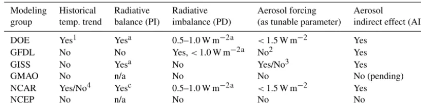
We summarize the results in Table 2. None of the models described here use the temperature trend over the historical period directly as a tuning target, nor are any of the mod-els tuned to set climate sensitivity to some preexisting as-sumption. However, NCAR, GFDL, and DOE do tune for a global radiative imbalance at near-present-day conditions. For instance, GFDL AM3 with observed SSTs was tuned to have a positive imbalance, with a magnitude less than about 1 W m−2for 1981–2000.

As discussed above, the radiative imbalance can be af-fected in two ways: by adjusting internal parameters (mostly associated with clouds) and/or by using a different historical forcing. Four models adjust their historical aerosol forcing: GISS, though only in its noninteractive runs, aims for an in-direct aerosol forcing of−1 W m−2 (Schmidt et al., 2014); NCAR CESM and DOE ACME tune for a substantive posi-tive effecposi-tive radiaposi-tive forcing at near-present conditions (im-plying a limit of−1.5 W m−2for aerosols); GFDL AM3 con-strained its ratio of Cess sensitivity to RFP to be close to its value in its prior-generation coupled model, which implied an aerosol forcing around−1.6 W m−2in AM3.

Table 2.Use of historical period trends and imbalances during the tuning process.

Modeling Historical Radiative Radiative Aerosol forcing Aerosol

group temp. trend balance (PI) imbalance (PD) (as tunable parameter) indirect effect (AIE)

DOE Yes1 Yesa 0.5–1.0 W m−2a <1.5 W m−2 Yes

GFDL No No Yes,<1.0 W m−2a No2 Yes

GISS No Yesa No Yes/No3 Yes

GMAO No n/a No No No (pending)

NCAR Yes/No4 Yesc 0.5–1.0 W m−2a <1.5 W m−2 Yes

NCEP No n/a No No No

a_{Using atmosphere-only or AMIP simulations.}c_{Using coupled ocean–atmosphere simulations.}1_{PD has to be warmer than PI.}2_However,

sensitivity and forcing were jointly constrained with respect to the previous model.3_{Set in simulations with noninteractive composition only.}4_It

was a necessary criteria for CCSM4, but not specifically tuned for. n/a=not applicable

model simulations are unclear. For example in the GISS-E2 model, the decadal mean imbalance (1996–2005) in AMIP simulations, including all forcings and annually varying ob-served SST and sea ice, is 1.25 W m−2 (for 1981–2000 it is 0.6 W m−2). However, using the decadal mean SST and sea ice for the same period and constant year-2000 forc-ings, the imbalance is much larger, at 1.74 W m−2. Further-more, the decadal mean imbalance in coupled simulations with the same forcings is ≈1.0±0.1 W m−2(Miller et al., 2014). Similarly, for the GFDL AM3 AMIP runs from 1981 to 2000, the radiative imbalance is 0.8 W m−2, while the im-balance for the same period in the coupled historical runs has an ensemble mean of 0.4 W m−2_{. The differences}

de-pend critically on the patterns of SST and sea ice, related to both the rectification of interannual variability and the offsets in the coupled model climatology compared to observations. The question that is raised by this is whether, given the in-crease in forcings over the historical period and the sensitiv-ity each model has, tuning the present-day imbalance (how-ever defined) determines (even to zeroth order) the coupled imbalance, the “committed warming” (at constant concen-trations) for the model, or the historical trend. With a perfect coupled model, and perfect knowledge of the forcings, this might be the case, but the imperfections in both imply that tuning to the PD imbalance is less of a constraint than might be assumed.

5 Discussion and future approaches

As models are continually evaluated at the process-level against an increasing number of observations, analyses often show that existing parameterizations lack enough flexibility to represent the coupling between the subgrid scale and the environment in all relevant climate regimes. The response is often to increase the complexity of a parameterization, which comes at the cost of an increased number of tunable param-eters. With that increase, the challenges faced by the devel-opers also rise, as does the potential for “local minima” to occur, i.e., different parameter combinations have similarly

good agreement according to standard GCM validation met-rics (e.g., Taylor diagrams, climate state mean biases, spatial correlations).

If these distinct and separate volumes of tuning parameter space lead to simulations that exhibit similarly good agree-ment with observations, there is no clear scientific reason to prefer one over another. But will our decisions on parameter combinations today have a noticeable impact on the simu-lated climate several centuries from now or to climate sen-sitivity more broadly? Specifically, does choosing different local minima in parameter phase space “matter”?

With more combinations, is there room for improving re-gional biases in simulations while simultaneously making the tuning process more automated? These questions have mo-tivated an effort, using the GISS model as a test bed, for developing a more robust framework for assessing the true existence of local minima in a multidimensional space (see also Hourdin et al., 2017). This is being explored by incorpo-rating situational or regime-dependent errors in observations or regional biases in GCM fields in weighted cost functions that define model “goodness”. We hope that this endeavor will increase the objectivity for deciding on the most appro-priate tuning parameters and either lead to improved met-rics for diagnosing the fidelity of a particular model or reveal the spread in simulated climate sensitivity arising from set-tling on very different, but seemingly optimal, combinations of tuning parameters.

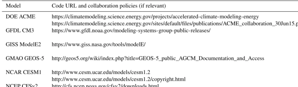
Table 3.Code availability at each center.

Model Code URL and collaboration policies (if relevant)

DOE ACME https://climatemodeling.science.energy.gov/projects/accelerated-climate-modeling-energy

https://climatemodeling.science.energy.gov/sites/default/files/publications/ACME_collaboration_30Jun15.pdf GFDL CM3 https://www.gfdl.noaa.gov/modeling-systems-group-public-releases/

GISS ModelE2 https://www.giss.nasa.gov/tools/modelE/

GMAO GEOS-5 http://geos5.org/wiki/index.php?title=GEOS-5_public_AGCM_Documentation_and_Access

NCAR CESM1 http://www.cesm.ucar.edu/models/cesm1.2

http://www.cesm.ucar.edu/models/cesm1.2/copyright.html NCEP CFSv2 http://cfs.ncep.noaa.gov/cfsv2/downloads.html

about an unstructured multimodel ensemble (see, e.g., Knutti et al., 2010, 2013).

At the minimum, we recommend that all future model de-scription papers (or systematic documentation projects such as ES-DOC http://es-doc.org) include a list of tuned-for tar-gets and monitored diagnostics and describe clearly (as in Table 2) their use of historical trends and imbalances in the development process.

While we have only discussed tuning in the context of his-torical and modern simulations, it is vital to assess the cred-ibility of models by examining their performance in out-of-sample situations. This is easy for the models with an oper-ational weather forecast mode (at least for some aspects of the climate system), and participation in paleoclimate model tests by NCAR and GISS are also invaluable. Medium-term climate forecasts based on anticipated changes in forcings (such as the eruption of Mount Pinatubo (1991) or the rise in greenhouse gases) have been shown to have skill (Hansen et al., 1988, 1992; Hargreaves, 2010). The importance (or lack thereof) of tuning always needs to be seen within that context. This paper alone cannot hope to answer all of the above questions, but we hope that it can contribute to a more transparent and more widely usable discussion.

Code and data availability. The availability of code for the models discussed in this paper is laid out in Table 3, though note that some decisions and/or tunings mentioned above are associated with cur-rent development which may only be accessible with a collaborative agreement in place.

Competing interests. The authors declare that they have no conflict of interest.

Acknowledgements. Climate modeling at GISS and GMAO is supported by the NASA Modeling, Analysis and Prediction program and resources supporting this work were provided by the NASA High-End Computing (HEC) Program through the NASA

Center for Climate Simulation (NCCS) at Goddard Space Flight Center. Work at LLNL was supported by the U.S. Department of Energy, Office of Science E3SM project under contract DE-AC52-07NA27344. NCEP is a division of the National Weather Service in NOAA within the Department of Commerce. Discussions at the US Climate Modeling Summit, convened by USGCRP in February 2016, were instrumental for putting this paper together. Manuscript reviews by Larry Horowitz and Levi Silvers (GFDL) are appreciated. We would like to thank Steve Sherwood and an anonymous reviewer for constructive comments on the discussion version of the paper.

Edited by: James Annan

Reviewed by: Steven Sherwood and one anonymous referee

References

Alexander, M. and Dunkerton, T.: A spectral parameterization of mean-flow forcing due to breaking gravity waves, J. Atmos. Sci., 56, 4167–4182, 1999.

Allan, R. P., Liu, C., Loeb, N. G., Palmer, M. D., Roberts, M., Smith, D., and Vidale, P.-L.: Changes in global net radiative imbalance 1985–2012, Geophys. Res. Lett., 41, 5588–5597, https://doi.org/10.1002/2014gl060962, 2014.

Annan, J. D. and Hargreaves, J. C.: On the meaning of inde-pendence in climate science, Earth Syst. Dynam., 8, 211–224, https://doi.org/10.5194/esd-8-211-2017, 2017.

Benedict, J., Maloney, E., Sobel, A., Frierson, D., and Don-ner, L.: Tropical intraseasonal variability in Version 3 of the GFDL atmosphere model, J. Climate, 26, 426–449, https://doi.org/10.1175/JCLI-D-12-00103.1, 2013.

Bi, D., Dix, M., Marsland, S., O’Farrell, S., Rashid, H., Uotila, P., Hirst, A., Kowalczyk, E., Golebiewski, M., Sullivan, A., Yan, H., Hannah, N., Franklin, C., Sun, Z., Vohralik, P., Watterson, I., Zhou, X., Fiedler, R., Collier, M., Ma, Y., Noonan, J., Stevens, L., Uhe, P., Zhu, H., Griffies, S., Hill, R., Harris, C., and Puri, K.: The ACCESS coupled model: description, control climate and evaluation, Aust. Met. Oceanogr. J., 63, 41–64, 2013.

J. Climate, 26, 9655–9676, https://doi.org/10.1175/JCLI-D-13-00075.1, 2013.

Bosilovich, M. G.: Regional Climate and Variability of NASA MERRA and Recent Reanalyses: U.S. Summertime Precipita-tion and Temperature, J. Appl. Meteorol. Clim., 52, 1939–1951, https://doi.org/10.1175/jamc-d-12-0291.1, 2013.

Bretherton, C., McCaa, J., and Grenier, H.: A new parameteriza-tion for shallow cumulus parameterizaparameteriza-tion and its applicaparameteriza-tion to marine subtropical cloud-topped boundary layers, Mon. Weather Rev., 132, 864–882, 2004.

Cess, R., Potter, G., Blanchet, J., Boer, G., Genio, A. D., Déqué, M., Dymnikov, V., Galin, V., Gates, W. L., Ghan, S. J., Kiehl, J. T., Lacis, A. A., Le Treut, H., Li, Z.-X., Liang, X.-Z., McAvaney, B. J., Meleshko, V. P., Mitchell, J. F. B., Morcrette, J.-J., Randall, D. A., Rikus, L., Roeckner, E., Royer, J. F., Schlese, U., Sheinin, D. A., Slingo, A., Sokolov, A. P., Taylor, K. E., Washington, W. M., Wetherald, R. T., Yagai, I., and Zhang, M.-H.: Intercompari-son and interpretation of climate feedback processes in 19 atmo-spheric general circulation models, J. Geophys. Res., 95, 16601– 16615, https://doi.org/10.1029/JD095iD10p16601, 1990. Church, J. A., White, N. J., Konikow, L. F., Domingues, C. M.,

Cog-ley, J. G., Rignot, E., Gregory, J. M., van den Broeke, M. R., Monaghan, A. J., and Velicogna, I.: Revisiting the Earth’s sea-level and energy budgets from 1961 to 2008, Geophys. Res. Lett., 38, L18601, https://doi.org/10.1029/2011GL048794, 2011. Del Genio, A. D., Wu, J., Wolf, A. B., Chen, Y., Yao, M.-S., and

Kim, D.: Constraints on Cumulus Parameterization from Sim-ulations of Observed MJO Events, J. Climate, 28, 6419–6442, https://doi.org/10.1175/jcli-d-14-00832.1, 2015.

Dessler, A. E. and Davis, S. M.: Trends in tropospheric humid-ity from reanalysis systems, J. Geophys. Res., 115, D19127, https://doi.org/10.1029/2010jd014192, 2010.

Donner, L.: A cumulus parameterization including mass fluxes, vertical momentum dynamics, and mesoscale effects, J. Atmos. Sci., 50, 889–906, https://doi.org/10.1175/1520-0469(1993)050<0889:ACPIMF>2.0.CO;2, 1993.

Donner, L. J., Wyman, B., Hemler, R., Horowitz, L., Ming, Y., Zhao, M., Golaz, J.-C., Ginoux, P., Lin, S., Schwarzkopf, M. D., Austin, J., Alaka, G., Cooke, W. F., Delworth, T. L., Freidenre-ich, S. M., Gordon, C. T., Griffies, S. M., Held, I. M., Hurlin, W. J., Klein, S. A., Knutson, T. R., Langenhorst, A. R., Lee, H., Lin, Y., Magi, B. I., Malyshev, S. L., Milly, P. C., Naik, V., Nath, M. J., Pincus, R., Ploshay, J. J., Ramaswamy, V., Se-man, C. J., Shevliakova, E., Sirutis, J. J., Stern, W. F., Stouffer, R. J., Wilson, R. J., Winton, M., Wittenberg, A. T., and Zeng, F.: The dynamical core, physical parameterizations, and basic simulation characteristics of the atmospheric component of the GFDL global coupled model CM3, J. Climate, 24, 3484–3519, https://doi.org/10.1175/2011JCLI3955.1, 2011.

Feingold, G.: Modeling of the first indirect effect: Analysis of measurement requirements, Geophys. Res. Lett., 30, 1997, https://doi.org/10.1029/2003GL017967, 2003.

Flato, G., Marotzke, J., Abiodun, B., Braconnot, P., Chou, S. C., Collins, W., Cox, P., Driouech, F., Emori, S., Eyring, V., Forest, C., Gleckler, P., Guilyardi, E., Jakob, C., Kattsov, V., Reason, C., and Rummukaine, M.: Evaluation of Climate Models, in: Cli-mate Change 2013: The Physical Science Basis. Contribution of Working Group I to the Fifth Assessment Report of the Intergov-ernmental Panel on Climate Change, edited by: Stocker, T. F.,

Qin, D., Plattner, G.-K., Tignor, M., Allen, S. K., Boschung, J., Nauels, A., Xia, Y., Bex, V., and Midgley, P., Cambridge Uni-versity Press, Cambridge, United Kingdom and New York, NY, USA, 2013.

Forster, P. M., Andrews, T., Good, P., Gregory, J. M., Jackson, L. S., and Zelinka, M.: Evaluating adjusted forcing and model spread for historical and future scenarios in the CMIP5 gener-ation of climate models, J. Geophys. Res.-Atmos., 118, 1139– 1150, https://doi.org/10.1002/jgrd.50174, 2013.

Gelaro, R., McCarty, W., Suárez, M. J., Todling, R., Molod, A., Takacs, L., Randles, C. A., Darmenov, A., Bosilovich, M. G., Re-ichle, R., Wargan, K., Coy, L., Cullather, R., Draper, C., Akella, S., Buchard, V., Conaty, A., da Silva, A. M., Gu, W., Kim, G., Koster, R., Lucchesi, R., Merkova, D., Nielsen, J. E., Partyka, G., Pawson, S., Putman, W., Rienecker, M., Schubert, S. D., Sienkiewicz, M., and Zhao, B.: The Modern-Era Retrospective Analysis for Research and Applications, Version-2 (MERRA-2), J. Climate, 30, 5419–5454, https://doi.org/10.1175/JCLI-D-16-0758.1, 2016.

Gent, P. R., Danabasoglu, G., Donner, L. J., Holland, M. M., Hunke, E. C., Jayne, S. R., Lawrence, D. M., Neale, R. B., Rasch, P. J., Vertenstein, M., Worley, P. H., Yang, Z.-L., and Zhang, M.: The Community Climate System Model Version 4, J. Climate, 24, 4973–4991, https://doi.org/10.1175/2011jcli4083.1, 2011. The GFDL Global Atmospheric Model Development Team: The

new GFDL global atmosphere and land model AM2-LM2: Eval-uation with prescribed SST simulations, J. Climate, 17, 4641– 4673, https://doi.org/10.1175/JCLI-3223.1, 2004.

Golaz, J.-C., Salzmann, M., Donner, L., Horowitz, L., Ming, Y., and Zhao, M.: Sensitivity of the Aerosol Indirect Effect to Subgrid Variability in the Cloud Parameterization of the GFDL Atmo-sphere General Circulation Model AM3, J. Climate, 24, 3145– 3160, https://doi.org/10.1175/2010JCLI3945.1, 2011.

Golaz, J.-C., Horowitz, L., and Levy II, H.: Cloud tuning in a cou-pled climate model: Impact on 20th century warming, Geophys. Res. Lett., 40, 2246–2251, https://doi.org/10.1002/grl.50232, 2013.

Griffies, S., Winton, M., Donner, L., Horowitz, L., Downes, S., Far-neti, R., Gnanadesikan, A., Hurlin, W. J., Lee, H., Liang, Z., Pal-ter, J. B., Samuels, B. L., Wittenberg, A. T., Wyman, B. L., Yin, J., and Zadeh, N.: GFDL’s CM3 coupled climate model: Char-acteristics of the ocean and sea ice simulations, J. Climate, 24, 3520–3544,https://doi.org/10.1175/2011JCLI3964.1, 2011. Griffies, S. M., Biastoch, A., Böning, C., Bryan, F., Danabasoglu,

G., Chassignet, E. P., England, M. H., Gerdes, R., Haak, H., Hallberg, R. W., Hazeleger, W., Jungclaus, J., Large, W. G., Madec, G., Pirani, A., Samuels, B. L., Scheinert, M., Gupta, A. S., Severijns, C. A., Simmons, H. L., Treguier, A. M., Winton, M., Yeager, S., and Yin, J.: Coordinated Ocean-ice Reference Experiments (COREs), Ocean Model., 26, 1–46, https://doi.org/10.1016/j.ocemod.2008.08.007, 2009.

Hansen, J., Fung, I., Lacis, A., Rind, D., Lebedeff, S., Ruedy, R., Russell, G., and Stone, P.: Global climate changes as forecast by Goddard Institute for Space Studies three-dimensional model, J. Geophys. Res., 93, 9341–9364, 1988.